RESEARCH ARTICLE
10.1002/2017JC012857
Three-Dimensional Sediment Dynamics in Well-Mixed
Estuaries: Importance of the Internally Generated Overtide,
Spatial Settling Lag, and Gravitational Circulation
Xiaoyan Wei1,2 , Mohit Kumar1, and Henk M. Schuttelaars1
1Applied Mathematics, Delft University of Technology, Delft, the Netherlands,2Now at National Oceanography Centre,
Liverpool, UK
Abstract
To investigate the dominant sediment transport and trapping mechanisms, a semi-analytical three-dimensional model is developed resolving the dynamic effects of salt intrusion on sediment in well-mixed estuaries in morphodynamic equilibrium. As a study case, a schematized estuary with a converg-ing width and a channel-shoal structure representative for the Delaware estuary is considered. When neglecting Coriolis effects, sediment downstream of the estuarine turbidity maximum (ETM) is imported into the estuary through the deeper channel and exported over the shoals. Within the ETM region, sediment is transported seaward through the deeper channel and transported landward over the shoals. The largest contribution to the cross-sectionally integrated seaward residual sediment transport is attributed to the advection of tidally averaged sediment concentrations by river-induced flow and tidal return flow. This contribution is mainly balanced by the residual landward sediment transport due to temporal correlations between the suspended sediment concentrations and velocities at theM2tidal frequency. TheM2sedimentconcentration mainly results from spatial settling lag effects and asymmetric bed shear stresses due to inter-actions ofM2bottom velocities and the internally generatedM4tidal velocities, as well as the
salinity-induced residual currents. Residual advection of tidally averaged sediment concentrations also plays an important role in the landward sediment transport. Including Coriolis effects hardly changes the cross-sectionally integrated sediment balance, but results in a landward (seaward) sediment transport on the right (left) side of the estuary looking seaward, consistent with observations from literature. The sediment transport/trapping mechanisms change significantly when varying the settling velocity and river discharge.
1. Introduction
An estuarine turbidity maximum (ETM) is a region where the suspended sediment concentration is ele-vated compared to concentrations upstream or downstream of that region. Estuarine turbidity maxima can have strong implications for estuarine morphology, ecology and biology, because of a continuous deposition of particulate matter that often contains contaminants (de Jonge et al., 2014; Jay & Musiak, 1994; Jay et al., 2015; Lin & Kuo, 2003; Sanford et al., 2001; Schoellhamer et al., 2007). Furthermore, these high turbidity levels result in reduced light availability and oxygen levels (de Jonge et al., 2014; McSwee-ney et al., 2016a; Talke et al., 2009). ETM’s are often located at regions of low salinities (Grabemann et al., 1997), but they can also be found in regions with larger salinities (Gibbs et al., 1983; Lin & Kuo, 2001) or even at fixed locations independent of salinity (Jay & Musiak, 1994; Lin & Kuo, 2001). This large variability in sediment trapping locations highlights the importance to identify the dominant mechanisms resulting in the ETM formation.
Process-based models have been intensively used to investigate sediment transport and trapping. Complex process-based models (see e.g., Ralston et al., 2012; Van Maren et al., 2015) are often used to investigate a specific estuary in detail. These models take into account observed estuarine bathymetry, geometry and forcing conditions and include all known physical processes and state-of-the-art parameterizations, thus allowing for a quantitative comparison of the model results with observations. Due to their complexity, these models are often solved numerically, which complicates the assessment of the influence of physical mechanisms in isolation. Furthermore, due to their long run-time, these models are not commonly used for systematic sensitivity studies.
Key Points:
Transport ofM2suspended sediment
concentrations byM2velocities
dominates the landward transport in the idealized Delaware estuary
Coarse sediments are mostly trapped in the channel near the salt intrusion limit while fine sediments mostly trapped on downstream shoals
The influence of gravitational circulation on sediment transport increases significantly with increasing river discharge
Correspondence to: X. Wei,
xywei1988@hotmail.com
Citation:
Wei, X., Kumar, M., & Schuttelaars, H. M. (2018). Three-dimensional sediment dynamics in well-mixed estuaries: importance of the internally generated overtide, spatial settling lag, and gravitational circulation.Journal of Geophysical Research: Oceans,123. https://doi.org/10.1002/2017JC012857
Received 3 MAR 2017 Accepted 12 DEC 2017
Accepted article online 27 DEC 2017
VC2017. The Authors.
This is an open access article under the terms of the Creative Commons Attri-bution-NonCommercial-NoDerivs License, which permits use and distri-bution in any medium, provided the original work is properly cited, the use is non-commercial and no modifica-tions or adaptamodifica-tions are made.
Journal of Geophysical Research: Oceans
PUBLICATIONS
Idealized process-based models, which focus on specific processes using idealized geometries and bathyme-tries, are effective tools to systematically investigate the dominant trapping mechanisms and study the sensi-tivity of these mechanisms to model parameters. Idealized models have been developed to investigate the cross-sectionally averaged (1-D) processes (Friedrichs et al., 1998; De Swart & Zimmerman, 2009; Winterwerp, 2011), width-averaged (longitudinal-vertical, 2DV) processes (Burchard & Baumert, 1998; Chernetsky et al., 2010; de Jonge et al., 2014; Geyer, 1993; Jay & Musiak, 1994; Schuttelaars et al., 2013; Talke et al., 2009), or lat-eral processes assuming along-channel uniform conditions (Huijts et al., 2006, 2011; Yang et al., 2014). The results of the width-averaged models show that the formation and maintenance of the ETM can often be attributed to the convergence of residual seaward sediment transport upstream of the ETM induced by river discharge, and residual landward sediment transport downstream of the ETM resulting from various mecha-nisms. These mechanisms include the salinity-induced gravitational circulation (Festa & Hansen, 1978; Postma, 1967), settling lag effects and tidal asymmetry (Chernetsky et al., 2010; De Swart & Zimmerman, 2009; Frie-drichs et al., 1998; Lin & Kuo, 2001; Winterwerp & Wang, 2013), tidal straining (Burchard & Baumert, 1998; Burchard et al., 2004; Scully & Friedrichs, 2007), stratification induced by salinity (Geyer, 1993) or sediment con-centration (Winterwerp, 2011), sediment-induced currents (Talke et al., 2009), flocculation and hindered settling (Winterwerp, 2011). Focusing on the lateral sediment trapping mechanisms, Huijts et al. (2006, 2011) showed that the lateral density gradient was crucial for the lateral sediment trapping, while trapping due to the Coriolis effects was less important. Extending the work of Huijts et al. (2006, 2011), Yang et al. (2014) found that the effects of the lateral density gradient,M4tidal flow and spatial settling lag all played an important role in the
lateral sediment trapping. The above-mentioned references clearly show that most idealized models either focus on longitudinal or lateral processes, even though observational studies have shown that both lateral and longitudinal processes, and especially their interaction, can be important to the along-channel and cross-channel sediment transport and trapping in estuaries (Becherer et al., 2016; Fugate et al., 2007; McSweeney et al., 2016b; Sommerfield & Wong, 2011). To investigate the importance of the three-dimensional (3-D) sedi-ment trapping mechanisms, Kumar et al. (2017) developed a semi-analytical three-dimensional model combin-ing the longitudinal and lateral approaches of Chernetsky et al. (2010) and Huijts et al. (2006) in a consistent way. However, the resulting model is still diagnostic in salinity, thus the dynamic effects of salinity-induced gravitational circulation on sediment transport and trapping, which are potentially important, are not included. The aim of this paper is to develop a three-dimensional semi-analytical model that allows for a systematical analysis of the sediment trapping and transport mechanisms, explicitly resolving the dynamic effects of salinity. Flocculation effects are ignored by considering only noncohesive sediments. First, the coupled water motion and salinity are obtained. Using this information, the sediment transport and distribution are calculated. This approach allows for a systematical analysis of the three-dimensional sediment trapping mechanisms and the importance of each individual mechanism for the ETM formation. In this paper, a sche-matized estuary is considered, with characteristics representative for the Delaware estuary, in which both lateral and longitudinal circulations are significant (McSweeney et al., 2016a, 2016b). Moreover, since the location of sediment trapping can change significantly with varying settling velocity and river discharge (Aubrey, 1986; de Jonge et al., 2014; Jay et al., 2015; Uncles & Stephens, 1993), a sensitivity study of the three-dimensional sediment trapping locations and mechanisms for these two factor is conducted.
The structure of this paper is as follows: in section 2, the idealized model is introduced, including the gov-erning equations and corresponding boundary conditions (section 2.1), a brief introduction of the adopted semi-analytical method (section 2.2) and an analytical decomposition of the sediment transport mecha-nisms (section 2.3). In section 3, the default experiment using parameters representative for the Delaware estuary, but neglecting Coriolis effects, is studied to show the 3-D sediment trapping mechanisms. The influence of Coriolis deflection is investigated in section 4. Next, a sensitivity study of the sediment trapping mechanisms for the sediment settling velocity and river discharge is presented in section 5. The above-mentioned sensitivity and the limitations of the present idealized model are discussed in section 6. Some conclusions are drawn in section 7.
2. Model Description
The semi-analytical idealized three-dimensional (3-D) model presented in this paper consists of the shallow water equations, dynamically coupled to the salinity module described in Wei et al. (2017) and to the
sediment module of Kumar et al. (2017). The estuary is assumed to be well-mixed and tidally dominated. Since the coupled water motion and salinity are calculated simultaneously, the salinity effects on the water motion and sediment transport are dynamically obtained.
In section 2.1, the systems of equations governing the water motion, salinity and sediment dynamics, together with the corresponding boundary conditions are introduced; the solution method is briefly intro-duced in section 2.2; the analytical decomposition of the sediment transport mechanisms is introintro-duced in section 2.3.
2.1. Governing Equations and Boundary Conditions
The estuary under consideration is forced by tides at the seaward boundary (@SX) and a river discharge at the landward boundary (@RX), where a weir is located (see Figure 1). The closed boundaries (@CX) are imper-meable. The undisturbed water level is located atz50, and the free surface elevation is denoted byz5g. The estuarine bathymetry varies in the horizontal directionsz52Hðx;yÞ, withHan arbitrary function of the horizontal coordinates (x,y).
The water motion is governed by the 3-D shallow water equations assuming hydrostatic equilibrium and using the Boussinesq approximation:
@u @x1 @v @y1 @w @z50; (1) @u @t1䉮 ðUuÞ2fv52g @g @x2 g qc ðg z @q @xdz1 @ @z Av @u @z ; (2) @v @t1䉮 ðUvÞ1fu52g @g @y2 g qc ðg z @q @ydz1 @ @z Av @v @z : (3)
Heretdenotes time,U5ðu;v;wÞis the velocity vector, withu,vandwthe velocity components inx,yandz directions, respectively. The acceleration of gravity is denoted byg, with a value of 9.8 m2s21.A
vis the
ver-tical eddy viscosity coefficient. Following Winant (2008) and Kumar et al. (2017), the horizontal viscous effects are neglected. The Coriolis parameter is denoted byf. The estuarine water densityqis assumed to depend only on the salinitySasq5qcð11bsSÞ, withbs57.631024psu21andq
cthe background density,
taken to be 1,000 kgm23. To dynamically calculate the density, the salinity equation needs to be solved:
@S @t1䉮 ðUSÞ5 @ @x Kh @S @x 1@ @y Kh @S @y 1@ @z Kv @S @z ; (4)
withKhandKv(assumed to be equal toAv) the horizontal and vertical
diffusivity coefficients, respectively. The suspended sediment concen-tration (SSC) equation reads
@C @t1䉮 ðUCÞ2 @ðwsCÞ @z 5 @ @x Kh @C @x 1 @ @y Kh @C @y 1@ @z Kv @C @z ; (5) where wsis the sediment settling velocity and strongly depends on
the sediment grain size (Fredsøe & Deigaard, 1992).
At the closed boundaries, @CX, the normal depth-integrated water flux and the tidally averaged salt and sediment transports are required to vanish. At the river boundary@RX, a river dischargeQis prescribed, while the normal tidally averaged salt and sediment transports have to vanish, for details see Wei et al. (2017) and Kumar et al. (2017). At the seaward boundaries, the water motion is forced by a prescribed Figure 1.A three-dimensional sketch of the estuary, withxandythe horizontal
coordinates, andzthe vertical coordinate, positive in the upward direction. The seaward, river, and closed boundaries are denoted by@SX; @RX,and@CX,
respectively. The free surface elevation and the estuarine bottom are located at
sea surface elevation that consists of a semi-diurnal tidal constituent (M2), its first overtide (M4), and a
resid-ual sea surface elevation (M0):
gðx;y;tÞ5aM2ðx;yÞcos½rM2t2uM2ðx;yÞ1aM4ðx;yÞcos½2rM2t2uM4ðx;yÞ1aM0ðx;yÞ atðx;yÞ 2@SX; (6)
whereaM2;aM4;uM2 anduM4are the prescribed amplitude and phase of the semi-diurnal and its first over-tide at the seaward boundary@SX, respectively. HererM21:431024s21denotes theM2tidal frequency.
The prescribed residual sea surface elevated at@SXis denoted byaM0ðx;yÞ. The tidally averaged salinity and suspended sediment concentration are prescribed at@SX,
S5Seðx;yÞ; C5Cmðx;yÞ atðx;yÞ 2@SX; (7) with the overbardenoting a tidal average. Note that the seaward boundary condition for the sediment concentration in (7) is different from that used in Kumar et al. (2017), where the normal (depth-integrated) sediment transport is required to vanish at each location of the seaward boundary. Using boundary condi-tion (7) allows a pointwise nonzero sediment transport over the seaward boundary. In equilibrium, the cross-sectionally integrated sediment transport has to vanish due to the no-transport condition at the closed and river boundaries.
For the water motion, the kinematic and no stress boundary conditions are prescribed at the free surface (z5g): w5@g @t1u @g @x1v @g @y; (8) Av @u @z5Av @v @z50: (9)
At the bottom (z52H), the normal velocity is required to vanish and a partial slip condition is applied (Schramkowski & De Swart, 2002):
w52@H @xu2 @H @yv; (10) Av @u @z; @v @z 5s h b qc5sðu;vÞ: (11)
The slip parametersdepends on the bed roughness and follows from linearizing the horizontal component of the bed shear stresssh
b. Here the horizontal bed shear stress is used because the depth gradients are assumed to be small, thus the vertical component of the bed shear stress is negligible. Concerning the salin-ity dynamics, the salt flux is required to vanish at the free surface and the bottom.
The normal sediment flux is required to vanish at the surface,
Kh @C @x;Kh @C @y;Kv @C @z1wsC ~ng50 at z5g; (12)
with~ngthe normal vector at the free surface, pointing upward:~ng5 2@@gx;2
@g
@y;1
. The normal component of the diffusive sediment flux at the bottom is related to the erosion fluxE5wsCrefby
Kh @C @x;Kh @C @y;Kv @C @z ~nb5wsCref at z52Hðx;yÞ; (13) with~nb5 2@@Hx;2 @H @y;21
the normal vector at the bottom pointing downward. The reference concentra-tion is denoted byCref, and is proportional to the bed shear stress and the sediment availabilitya:
Cref5
qsajshbj q0g0d
s
: (14)
Hereqsdenotes the sediment density,g05gðqs2q0Þ=q0 the reduced gravity anddsthe sediment grain
size. The mean water densityq0takes into account the effects of salt on water density and is assumed to
be a constant. The sediment availabilityais an erosion coefficient that accounts for the amount of easily erodible sediment available in a mud reach (Chernetsky et al., 2010; Friedrichs et al., 1998; Huijts et al., 2006).
At this point, the sediment availabilityais still unknown. By assuming the estuary to be in morphodynamic equilibrium (the tidally averaged sediment deposition and erosion balance each other, for details, see Frie-drichs et al., 1998; Kumar et al., 2017), the spatial distribution ofafollows from solving the tidally averaged and depth-integrated sediment equation
@ @x ðg 2H Cu2Kh @C @x dz1 @ @y ðg 2H Cv2Kh @C @y dz50; (15)
using boundary conditions (7), (12), (13), and no normal sediment transport conditions at the closed and landward boundaries.
2.2. Solution Method
To identify the relative importance of different mechanisms governing the sediment dynamics, a semi-analytical approach is used to solve equations (1)–(15). In this approach, we employ a perturbation method to get an ordered system of equations which are partly solved analytically and partly numerically using a finite element method. The perturbation method is originally developed by Ianniello (1977) to derive ana-lytic solutions for the width-averaged tidally induced residual currents, which was later used in McCarthy (1993) to calculate the width-averaged density-induced residual currents in well-mixed estuaries. As a first step of the perturbation method, all physical variables are scaled by their typical values, resulting in a nondi-mensional system of equations. The dimensionless numbers that indicate the relative importance of the var-ious terms are then compared to the small parameterE, withEthe ratio between theM2tidal amplitude to
the water depth averaged over the seaward boundary. Next, terms of the same order inEare collected, resulting in a system of equations at each order ofEthat can be solved separately. The vertical structure of all physical variables describing the water motion, salinity and sediment concentration are obtained analyti-cally, while their horizontal structures have to be calculated numerically. Here we use a finite element method (for details, see Kumar et al., 2016, 2017; Wei et al., 2017) to get the horizontal dependencies. Using this approach, the barotropic water motion, including the residual (M0) flow, and theM2andM4tidal flow
can be explicitly calculated. However, since the baroclinic residual flow (i.e., gravitational circulation) is dynamically coupled to salinity, an iterative approach is needed to simultaneously calculate the gravita-tional circulation and the salinity field (for details, see Wei et al., 2017). After calculating the necessary water motion constituents (M0, M2, M4), the suspended sediment concentration at each order of E can be
expressed in terms of the sediment availability, which follows from the morphodynamic equilibrium condi-tion (Kumar et al., 2017).
2.3. An Analytical Decomposition
Using the solution method sketched above and neglecting terms ofOðE2Þand higher, the flow velocity can be analytically decomposed into two tidal constituents and a residual component:
U5UM2 |{z} Oð1Þ 1UM41UM0 |fflfflfflfflfflffl{zfflfflfflfflfflffl} OðEÞ : (16)
HereUM2 is the leading-order tidal velocity vector at theM2tidal frequency (atOð1ÞÞ,UM4 is the first-order tidal velocity vector at theM4tidal frequency (atOðEÞ), andUM0 is theOðEÞsubtidal flow velocity vector. TheM2component of the flow velocityUM2 is externally forced by a prescribedM2tide at the entrance. Its
UM45UEFM41U AC M41U NS M41U TRF M4: (17) The first contributionUEF
M4 results from an externalM4forcing prescribed at the mouth, while other
con-tributions are generated internally by nonlinear interactions of theM2tidal constituent: tidal rectification
(UAC
M4), the stress-free condition (UNSM4, as the shear stress is required to vanish atz5ginstead ofz50) and tidal return flow (UTRF
M4). In this paper, tidal return flow (UTRFM4;UTRFM0) refers to the water flow associated with the Stokes’ drift and the return flow compensating theM4/M0component of the Stokes’ drift
contribu-tion. A more detailed explanation and formulation for different flow components can be found in section 5 of Kumar et al. (2017). The residual flowUM0 is analytically decomposed into different components as well:
UM05URDM01UGCM01UACM01UNSM01UTRFM0: (18)
HereURDM0 results from the externally prescribed river discharge. Other contributions are related to the salinity-induced gravitational circulation (UGC
M0), the nonlinear interactions due to tidal rectification (UACM0), the stress-free surface condition (UNS
M0) and tidal return flow (UTRFM0). In the asymptotic expansion, bothUM4 and
UM0are ofOðEÞ.
Substituting equation (16) into (11) and making a Taylor expansion with respect to the small parameterE, it follows thatjshbjcan be decomposed into Fourier series consisting of a residual component and all frequen-cies that are a multiple of theM2tidal frequency,
jshbj5qspuffiffiffiffiffiffiffiffiffiffiffiffiffi21v25 js bM0j1jsbM4j1jsbM8j1 |fflfflfflfflfflfflfflfflfflfflfflfflfflfflfflfflfflfflfflfflfflfflfflfflffl{zfflfflfflfflfflfflfflfflfflfflfflfflfflfflfflfflfflfflfflfflfflfflfflfflffl} Oð1Þ 1 jsbM2j1jsbM6j1 |fflfflfflfflfflfflfflfflfflfflfflfflfflfflfflfflffl{zfflfflfflfflfflfflfflfflfflfflfflfflfflfflfflfflffl} OðEÞ 1 (19)
Equation (19) shows that, when ignoring the difference in the amplitudes of different Fourier components, the residual bed shear stresssbM0, and all bed shear stresses of frequencies which are even multiples of the
M2tidal frequency (sbM4;sbM8,. . .) resulting from the M2bottom velocity, are leading-order contributions.
The other components (sbM2;sbM6,. . .) result from the interactions of theM2bottom velocity with the
resid-ual andM4bottom velocities, and are ofOðEÞ. From equations (13), (14), and (19), it follows that the
result-ing suspended sediment concentration is given by
C5ðCM01CM41CM81 Þ |fflfflfflfflfflfflfflfflfflfflfflfflfflfflfflfflfflffl{zfflfflfflfflfflfflfflfflfflfflfflfflfflfflfflfflfflffl} Oð1Þ 1ðCM21CM61 Þ |fflfflfflfflfflfflfflfflfflfflfflfflffl{zfflfflfflfflfflfflfflfflfflfflfflfflffl} OðEÞ 1 ; (20)
i.e., it consists of contributions at different tidal frequencies. It can be shown thatCM0;CM4 (andCM8,. . .) are leading-order concentrations, andCM2(andCM6,. . .) are first-order concentrations. However, equations (19) and (20) do not mean theM8(and higher) frequencies of the bed shear stress and SSC have to be as significant as the components atM0 andM4frequencies, because the amplitues ofM0andM4 compo-nents in the Fourier series are much larger than those ofM8and higher frequencies. The leading-order concentrations are induced by the bed shear stress due toM2bottom velocity. The first-order
concentra-tions, however, are caused both by the asymmetric bed shear due to the combinedM2andM0/M4bottom
velocities, and by the advection of the leading-order concentrations by theM2tidal velocity (UM2). More-over, the vanishing normal sediment flux prescribed at the free surface introduces a first-order sediment flux atz50, which also results in a first-order contribution in the sediment concentrationsCM2 (Kumar et al., 2017).
It is important to note that to obtain the dominant sediment transport balance, only the leading-order con-centrationsCM0andCM4, and the first-order concentrationCM2are needed. Using this information, substitut-ing equations (16), (18), (20) into (15), the depth-integrated, tidally averaged sediment transport equation becomes
䉮 ð0 2H uM0CM0dz1gM2uM2jz50CM0jz50 ð0 2H vM0CM0dz1gM2vM2jz50CM0jz50 0 B B B B @ 1 C C C C A |fflfflfflfflfflfflfflfflfflfflfflfflfflfflfflfflfflfflfflfflfflfflfflfflfflfflfflfflfflfflfflfflfflfflffl{zfflfflfflfflfflfflfflfflfflfflfflfflfflfflfflfflfflfflfflfflfflfflfflfflfflfflfflfflfflfflfflfflfflfflffl} TM0 1䉮 ð0 2H uM2CM2dz ð0 2H vM2CM2dz 0 B B B B @ 1 C C C C A |fflfflfflfflfflfflfflfflfflfflfflfflfflfflffl{zfflfflfflfflfflfflfflfflfflfflfflfflfflfflffl} TM2 1䉮 ð0 2H uM4CM4dz1gM2uM2jz50CM4jz50 ð0 2H vM4CM4dz1gM2vM2jz50CM4jz50 0 B B B B @ 1 C C C C A |fflfflfflfflfflfflfflfflfflfflfflfflfflfflfflfflfflfflfflfflfflfflfflfflfflfflfflfflfflfflfflfflfflfflffl{zfflfflfflfflfflfflfflfflfflfflfflfflfflfflfflfflfflfflfflfflfflfflfflfflfflfflfflfflfflfflfflfflfflfflffl} TM4 1䉮 2 ð0 2H Kh @CM0 @x dz 2 ð0 2H Kh @CM0 @y dz 0 B B B B @ 1 C C C C A |fflfflfflfflfflfflfflfflfflfflfflfflfflfflfflfflfflffl{zfflfflfflfflfflfflfflfflfflfflfflfflfflfflfflfflfflffl} TDIFF 50: (21)
In equation (21),TM0;TM2andTM4represent the depth-integrated residual sediment transport contributions due to different advective transport processes, andTDIFFdenotes transport due to diffusive processes. Here,
TM2 is the depth-integrated residual sediment transport due to the advection of theM2tidal concentration
CM2 byM2tidal velocities. The depth-integrated residual sediment transports due to the advection of the
residual concentrationCM0 by the residual velocities, and the advection of theM4tidal concentrationCM4 by theM4tidal velocities, are included inTM0 andTM4, respectively.
Following equations (17)–(20), the depth-integrated sediment transport contributions can be further decomposed into different mechanisms as listed in Table 1 (see a more detailed decomposition in Kumar et al., 2017). The sediment transportTM0 includes transport contributions due to the advection of the residual concentrationCM0 by the gravitational circulation (TGCM0), and the other barotropic residual flow components (TBRM0) as a result of the river-induced flow (TRDM0), tidal rectification (TACM0), the stress-free sur-face boundary condition (TNS
M0), and tidal return flow (TTRFM0). The depth-integrated transportTM2 includes theM2tidal advection of SSC at theM2tidal frequency, which is partly a result of the asymmetric bed
shear stress due to the interaction of theM2tidal velocity and the salinity-induced baroclinic residual
current (TGC
M2) and the internally generated barotropic residual current (TBRM2) at the bottom. Moreover, the asymmetric bed shear stress due to interactions of theM2 bottom velocity and the externally forced
(TEF
M2) or internally generated (TINM2)M4tidal currents at the bottom also induce anM2tidal concentration,
which temporally correlates with the M2 tidal velocity, and results in a residual sediment transport.
Besides, the first-order correction of the leading-order vertical sediment fluxes at the free-surface bound-ary results in a first-order SSC at theM2tidal frequency and thence a sediment transport (TSCM2), which is called the surface contribution (Kumar et al., 2017). Finally, the advection of the residual andM4tidal
components of SSC by theM2tidal currents also results in a SSC at theM2tidal frequency. Advection of
this concentration component by theM2 tidal currents again results in a residual sediment transport,
and is denoted as the spatial settling lag contribution (TSSLM2). The transport contributionTM4is caused by advection of SSC at theM4tidal frequency by theM4tidal flow as a result of both theM4tidal flow
gener-ated internally (TIN
M4) and the externally forced M4 tide (TEFM4). Owing to the semi-analytical solution method and the analytic approach of decomposition, all decomposed mechanisms listed above can be calculated individually.
Integrating equation (21) from the left bank of the channel (y5y1) to the right bank (y5y2), and subse-quently integrating from the weir (atx5L) to any longitudinal locationx, the cross-sectionally integrated longitudinal residual sediment balance is found:
ðy2 y1 ð0 2H uM0CM0dz1gM2uM2jz50CM0jz50 dy |fflfflfflfflfflfflfflfflfflfflfflfflfflfflfflfflfflfflfflfflfflfflfflfflfflfflfflfflfflfflfflfflfflfflfflfflfflfflffl{zfflfflfflfflfflfflfflfflfflfflfflfflfflfflfflfflfflfflfflfflfflfflfflfflfflfflfflfflfflfflfflfflfflfflfflfflfflfflffl} TM0 1 ðy2 y1 ð0 2H uM2CM2dzdy |fflfflfflfflfflfflfflfflfflfflfflfflfflfflffl{zfflfflfflfflfflfflfflfflfflfflfflfflfflfflffl} TM2 1 ðy2 y1 ð0 2H uM4CM4dz1gM2uM2jz50CM4jz50 dy |fflfflfflfflfflfflfflfflfflfflfflfflfflfflfflfflfflfflfflfflfflfflfflfflfflfflfflfflfflfflfflfflfflfflfflfflfflfflffl{zfflfflfflfflfflfflfflfflfflfflfflfflfflfflfflfflfflfflfflfflfflfflfflfflfflfflfflfflfflfflfflfflfflfflfflfflfflfflffl} TM4 1 ðy2 y1 ð0 2H 2Kh @CM0 @x dzdy |fflfflfflfflfflfflfflfflfflfflfflfflfflfflfflfflfflffl{zfflfflfflfflfflfflfflfflfflfflfflfflfflfflfflfflfflffl} TDIFF 50: (22)
Equation (22) shows that the cross-sectionally integrated along-channel residual sediment balance is main-tained byTM0;TM2;TM4, andTDIFF. These transport contributions can be further decomposed in the same way as the depth-integrated sediment transport contribution (not shown).
To analyze all potentially important processes which drive the transport and trapping of SSC in well-mixed estuaries, we will first consider a default experiment with parameter values representative for the Delaware estuary (neglecting Coriolis effects, see section 3). Then, the influence of the Coriolis effects on these pro-cesses will be investigated in section 4. After that, the sensitivity of these propro-cesses to the sediment settling velocity and river discharge will be analyzed (see section 5).
3. Default Experiment
The estuarine bathymetry, geometry, forcing conditions and parameters for the default experiment are defined in section 3.1. The resulting SSC structures in morphodynamic equilibrium and the depth-integrated sediment transport/trapping patterns are discussed in section 3.2 and 3.3, respectively. To under-stand the relative importance of various contributions to the along-channel residual sediment transport, the cross-sectinally integrated (along-channel) residual sediment balance is analyzed in section 3.4. The signifi-cance of sediment transports associated with the internally generated overtide, spatial settling lag effects and gravitational circulation to the ETM formation is investigated in section 3.5.
3.1. Parameters Setting for the Default Experiment
The default experiment considers a schematized, well-mixed estuary, with an estuarine length (L) of 215 km and a width (B) exponentially converging up-estuary,
B5B0e2x=Lb: (23)
HereB0539 km is the estuarine width at the mouth, andLb542 km the estuarine convergence length
(rep-resentative for the Delaware estuary). Following Wei et al. (2017), the bathymetry exhibits a lateral channel-shoal structure, and is given by
Hðx;yÞ5Hmin1ðHm2HminÞ x L1ðHmax2HminÞ 12 x L 124y 2 B2 e2Cf4y 2 B2; (24)
with the maximum water depthHmax515 m and the minimum water depthHmin53.6 m on the shoals of the estuarine mouth. The width-averaged water depthHm58 m and the tidal flat parameterCf54 are
con-stant along the channel. Table 1
Decomposition of the Depth-Integrated Sediment Transports Due to Different Contributionsa
Transport Decomposition Concentration Velocity
TM0 T GC M0 CM0 U GC M0 TRDM 0 U RD M0 TAC M0 U AC M0 TTRF M0 U TRF M0 TNS M0 U NS M0 TM2 TGCM2 CM2due toUM21U GC M0 UM2 TBR M2 CM2due toUM21U RD M01U AC M01U NS M01U TRF M0 TEF M2 CM2due toUM21U EF M4 TIN M2 CM2due toUM21U AC M41U NS M41U TRF M4 TSC
M2 CM2due to surface contribution
TSSL
M2 CM2due to spatial settling lag
TM4 TINM4 CM4 U AC M41U NS M41U TRF M4 TEF M4 U EF M4 a
In order to obtain a physically consistent solution for the salinity, and to make the sediment distribution at the seaward boundary consis-tent with that in the interior, the barotropic water motion will be cal-culated in a domain which is extended 30 km toward the open sea (see gray rectangle in Figure 2). A constant barotropic sea surface ele-vation is prescribed at the seaward boundary of the extended domain (x050) such that the width-averaged sea surface elevation gmat the
seaward boundary of the physical domain (x50)
gm5amM2cosðrM2tÞ1amM4cosð2rM2t2DumÞ1amM0 (25) is in agreement with the observations of the Delaware estuary by Wal-ters (1997). Here am
M2;amM4, andDum denote the width-averagedM2
andM4tidal amplitudes and the relative phase between theM2and
M4tidal constituents atx50, respectively. amM0 is the mean residual water level at x50, and is required to vanish. Following Wei et al. (2017), the residual salinity x50 (Sm) is prescribed to be 31 psu the
horizontal diffusivityKhis assumed to linearly decrease withB, from 50 m2s
21
at the mouth to 10 m2s21
at the landward side.
After calculating the barotropic water motion in the extended domain, the (baroclinic) gravitational circulation and salinity distribution are calculated for the domain of interest (betweenx50 andx5L). Then, using the resulting water motion, the sediment concentration for the (nonextended) domain of interest is calculated. The suspended sediment concentration at the seaward boundary of the physical domain (Cm) is prescribed to be a constant. The
value ofCmis determined by prescribing the averaged sediment availabilityain the physical domain
a5 ðL 0 ðy2 y1 a dydx ðL 0 ðy2 y1 dydx (26)
to be constant, such that a maximum residual SSC of200 mg L21representative for the observed ETM in the Delaware estuary under a relatively small river discharge (288 m3s21
; see McSweeney et al., 2016b) is obtained.
The vertical eddy viscosityAvis assumed to be constant in time. BothAvand the slip parameter sare
assumed to be proportional to the local water depth (Friedrichs & Hamrick, 1996; Wei et al., 2017), Av5Avm H Hm ; s5sm H Hm : (27)
HereHm is the width-averaged water depth, Avm andsm are prescribed friction parameters which are
obtained from calibrating theM2tidal water motion with observations in the Delaware estuary (values taken
from Wei et al., 2016). Using these parameter settings, the leading-order tidal surface elevation obtained from the present 3-D model is nearly the same as that obtained in their width-averaged model. The model qualitatively reproduces the observedM2tidal surface elevation and the three-dimensional flow structures
due to barotropic flow components and gravitational circulation. A discussion of the model performance on the water motion and salinity (transport) can be found in Wei et al. (2017), and is not repeated in this paper. The Delaware estuary is characterized by sediments of different grain-sizes which are distributed at different locations (Biggs & Church, 1984; Gibbs et al., 1983). For simplicity, a constant settling velocity value is used in the default experiment:ws50:5 mms21, representative for sediments in the lower Delaware Bay. To investigate the sediment dynamics for sediments of different settling velocities, two other settling velocities will be considered (ws50:2 mms21, 1 mms21) in the sensitivity study (see section 5.1). The grain size of sediments, the mean water density, and sediment density are also assumed to be constant:ds520lm,q05 1;020 kgm3,qs52;650 kgm3. For clarity, the Coriolis force is neglected in the default experiment, its effect will be discussed in detail in section 4. All above-mentioned parameters defining the default experiment are listed in Table 2.
Figure 2.The bathymetry and geometry of the extended domain, and the (nonextended) domain of interest.
3.2. Three-Dimensional Suspended Sediment Concentration
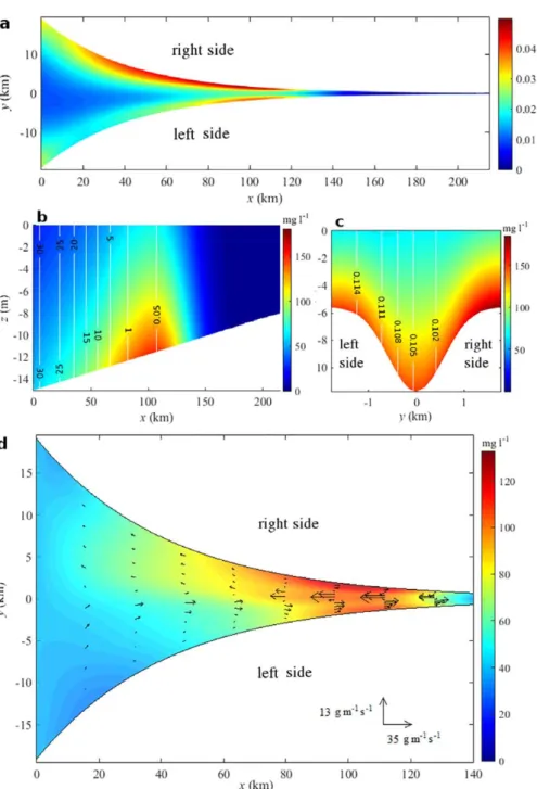
Since no Coriolis force is considered, and the bed profile and geometry are laterally symmetric, the sedi-ment availability and sedisedi-ment concentrations are symmetric with respect to the central axis of the estuary (y50). As shown in Figure 3a, the maximum sediment availability is found at about 100 km up-estuary from the mouth, with larger values on the shoals than in the deeper channel. To illustrate the three-dimensional structure of the ETM and its position with respect to the tidally averaged salinity structure, the longitudinal-vertical distribution of the residual suspended sediment concentration aty50 and a lateral-vertical (cross-sectional) distribution within the ETM region (atx5100 km) are depicted in Figures 3b and 3c. The residual salinity distributions are vertically uniform (see white lines), however, the residual sus-pended sediment concentrations are generally larger near the bottom than near the top (see color scales). The ETM is centered at100 km, with the turbidity zone stretching between 55 km and 130 km from the mouth (see Figure 3b). The maximum residual suspended sediment concentration is found at a salinity of about 0.05 psu, coinciding with the residual salt intrusion limit. Due to larger sediment availabilities on the shoals and larger residual salinities in the deeper channel (see Figure 3c), the residual suspended sediment concentrations are larger on the shoals than in the deeper channel (even though the bed shear stress in the deeper channel is larger). The lateral distributions of the residual salinity and suspended sediment concen-tration confirm the results of Huijts et al. (2006), that salinity gradients tend to trap sediment in regions of the cross section with lower salinities.
3.3. Depth-Integrated Sediment Transport and Trapping Mechanisms
To identify the longitudinal and lateral sediment transport patterns and the depth-averaged sediment trap-ping patterns, the depth-integrated residual sediment transport and the depth-averaged residual sediment concentration are shown in Figure 4. The maximum depth-averaged residual sediment concentration is located atx5100 km, with the depth-averaged ETM region extending from 70 to 120 km up-estuary from the mouth. Four circulation cells of residual sediment transport are identified (see arrows in Figure 4): sea-ward of the ETM, sediments are transported tosea-ward the ETM through the deeper channel, next move later-ally toward the flanks and are transported seaward over the shoal; within the ETM region, sediments are transported seaward through the deeper channel and landward over the shoals. The longitudinal residual sediment flux (integrated over the depth) reaches its maximum (up to 24 g m21s21) in the deeper channel
Table 2
Parameters for the Default Experiment
Physical Parameter Symbol Value
Length L 215 km
Convergence length Lb 42 km
Width at the mouth B0 39 km
Minimum water depth Hmin 3.6 m
Maximum water depth Hmax 15 m
Average water depth Hm 8 m
Tidal flat parameter Cf 4
Average vertical eddy viscosity Avm 0.005 m
2s21
Average slip parameter sm 0.039 ms21
Horizontal diffusivity Kh 10–50 m2s21
River discharge Q 288 m3s21
AverageM2tidal amplitude amM2 0.75 m
AverageM4tidal amplitude amM4 0.012 m
Average residual water level am
M0 0
M2tidal frequency rM2 1:431024s
21
Average phase difference Dum 2247
Coriolis parameter f 0
Salinity at the mouth Sm 31 psu
Mean water density q0 1,020 kgm23
Sediment grain size ds 20lm
Sediment density qs 2,650 kgm23
Settling velocity ws 0.5 mms21
within the ETM region at the central estuary, while the maximum lateral flux (less than 3 g m21s21) is found on the shoals near the mouth. To investigate the physical mechanisms behind the residual sediment trans-port and trapping, the depth-integrated residual sediment transtrans-port contributions due to advection of residual concentrations by residual velocities (TM0), advection of tidal components of sediment concentra-tions by tidal velocities (TM21TM4) and diffusive processes (TDIFF) are shown in Figure 5. The divergence (convergence) of the depth-integrated residual sediment transport due to each contribution is shown in blue (red), with the magnitude and direction of the sediment transport shown by arrows. Upstream of the seaward edge of the ETM, the residual sediment transport contributionTM0tends to transport sediment sea-ward. This results in a divergence of sediment transport in the upper estuary (x>120 km) and a conver-gence in the central region (70 km<x<120 km) of about 1 mg m22s21, see Figure 5a. Downstream of the ETM (x<70 km),TM0 tends to transport sediments landward through the deeper channel. Next, sediments are transported toward the flanks and subsequently exported over the shoals. This results in a strong diver-gence of sediment transport in the deeper channel (up to 3 mg m22s21) and a convergence on the shoals (up to 1 mg m22 s21). The residual sediment transport contributionsTM2 andTM4 represent the depth-integrated sediment transport due to the temporal correlations between sediment concentrations and velocities at theM2andM4tidal frequencies. These contributions, which are called tidal pumping
contribu-tion hereafter, significantly contributes to the depth-integrated residual sediment transport and trapping, withTM2 much larger thanTM4. The tidal pumping contribution plays an important role in transporting sedi-ments from the seaward side toward the ETM, while its contribution to the lateral sediment transport is neg-ligible (Figure 5b). Tidal pumping results in a divergence of sediment transport at the seaward side of the ETM and a convergence within the ETM region of less than 1 mg m22s21. Diffusive processes contribute to a transport of sediments from the shoals toward the deeper channel (Figure 5c), which is consistent with the model results that sediment concentrations are larger on the shoals than in the channel. As a result, the diffusive contribution results in a significant convergence of the depth-integrated residual sediment trans-port in the deeper channel (up to 3 mg m22s21) and a divergence on the shoals (up to 1 mg m22s21). Note that the divergence of the total depth-integrated residual sediment transport vanishes, as we assume the estuaries to be in morphodynamic equilibrium. It is clear that, downstream of the ETM, the landward Figure 3.(a) The spatial distribution of sediment availability. (b) The longitudinal-vertical profile aty50 and (c) lateral-vertical distributions of the residual concentration atx5100 km for the default experiment. The white contour lines show the vertically uniform residual salinities.
sediment transport in the deeper channel (see Figure 4) is mainly due toTM0 and tidal pumping, while the seaward sediment transport over the shoals is predominantly controlled byTM0.
To assess the relative importance of the advection of residual sediment concentrations by gravitational cir-culation (TGC
M0) and the other barotropic residual currents (TBRM0), the sediment transport due to these two con-tributions is shown in Figures 5d and 5e, respectively, together with the resulting divergence of the transport. It is found that the largest contribution to the divergence of the residual sediment transportTM0 in the seaward side of the ETM is related to the advection of the residual concentrations by the gravitational circulation (TGCM0). The convergence of the residual sediment transportTM0 on the shoals downstream of the ETM is due to the combined effects ofTGC
M0 andTBRM0. The convergence of the residual sediment transportTM0 in the ETM region, however, is mainly resulting from the advection of residual concentrations by the baro-tropic residual currents (TBR
M0) (see Figure 5e). The transport contributionTGCM0 tends to transport sediments landward through the deeper channel and seaward over the shoals (see Figure 5d). The contributionTBR
M0, however, transports sediments seaward at each location, especially in the deeper channel. In the deeper channel downstream of the ETM, the landward residual sediment transport contributionTGCM0 exceeds the seaward transport contributionTBR
M0; while on the shoals, bothTGCM0 andTBRM0 contribute to a seaward sedi-ment transport. As a result, the landward sedisedi-ment transport contributionTM0 in the deeper channel is smaller than the seaward transport on the shoals, as shown in Figure 5a.
3.4. Cross-Sectionally Integrated Residual Sediment Balance
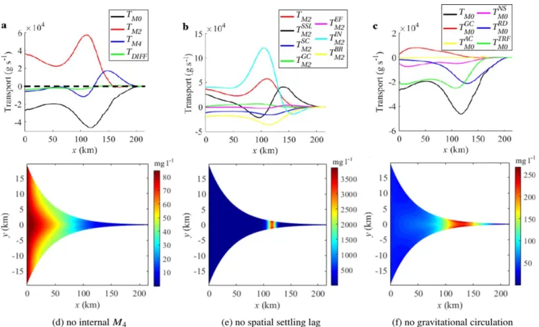
Integrating the sediment transport over the cross section results in the cross-sectionally integrated residual sediment transport balance due to different mechanisms. In Figure 6a, it is shown thatTM2 andTM0 are the dominant landward and seaward residual sediment transport contributions, respectively, while the residual sediment transport contributionsTM4andTDIFFare much smaller. This implies the dominant sediment trans-port processes are well-resolved by the idealized model. Since the horizontal diffusion tends to spread out sediments from the ETM, reducing horizontal diffusivity may slightly decrease the width of the ETM. To obtain the dominant sediment importing and exporting mechanisms, the sediment transport contributions TM2 andTM0 are further decomposed into contributions related to specific mechanisms listed in Table 1. The largest contribution to the landward residual sediment transport contributionTM2 is caused by theM2tidal
advection of the suspended sediment concentrations at theM2tidal frequency (TM2IN), as a result of the asym-metric bed shear stress due to interactions of theM2bottom velocity and the internally generatedM4
bot-tom velocity. TheM2 tidal advection of theM2tidal concentration as a result of the spatial settling lag
Figure 4.The averaged residual suspended sediment concentration (see background color scales) and the depth-integrated sediment flux (see arrows). The length of the arrow measures the magnitudes of the depth-depth-integrated residual suspended sediment flux at each location (x,y), and the direction of the arrow measures the direction of the flux at this location.
effects also results in a significant landward residual sediment transport contribution (TSSL
M2 ). The tidal advec-tion of the tidal concentraadvec-tions as a result of the asymmetric bed shear stress due to the combined salinity-induced bottom residual velocity and theM2bottom flow also contributes to a small but nonnegligible
landward sediment transport (TGC
M2). TheM2tidal advection of theM2tidal concentration as a result of the asymmetric bed shear stress due to interactions between theM2tidal velocities and the externally
gener-atedM4tidal velocities (TM2EF), however, is negligible for the residual sediment balance integrated over the cross section. TheM2tidal advection of theM2tidal concentration as a result of the asymmetric bed shear stress due to interactions between theM2 tidal velocities and the barotropic residual currents (TM2BR) and transport due to surface contribution (TSC
M2) result in a seaward residual transport of sediment. In Figure 6c, it is shown that the advection of the residual sediment concentration by gravitational circulation (TGC
M0) con-tributes to a landward sediment transport. The advection of residual sediment concentration by all Figure 5.The divergence of the depth-integrated residual sediment transport (see color scales) due to (a) residual advec-tion of residual concentraadvec-tions (TM0), (b) tidal pumping (TM21TM4), (c) diffusion (TDIFF), (d) transport due to advection of
residual suspended sediment concentration by gravitational circulation (TGC
M0), and (e) barotropic residual currents (T
BR M0).
barotropic residual velocities (TM0RD;TM0AC;TM0NS;TM0TRF), however, result in a seaward sediment transport contri-bution (see Figure 6c), withTRD
M0 andTM0TRFthe dominant seaward sediment transport contributions. 3.5. Contributions to the ETM
In this section, the significance of residual sediment transport contributions due toM2tidal advection of the
M2tidal concentration related to the internally generatedM4overtide, spatial settling lag effects, and the
residual andM2tidal advective transport by gravitational circulation to the ETM formation is studied. Three
dedicated experiments, in which one of these contributions is excluded, are used to show the differences of the characteristics of the resulting ETM in comparison with those in the default experiment. In these experi-ments, the sediments within the estuary have to be redistributed to reach a new morphodynamic equilib-rium, resulting in a changed sediment availability distribution and thus an altered ETM.
In experiments 1–2, the sediment transport contributions related to the internally generatedM4overtide
(TINM2) and the spatial settling lag effects (TSSLM2) are excluded, respectively. In both experiments, the ETM moves to the seaward boundary (see Figures 7a and 7b). This implies that bothTIN
M2 andTSSLM2 are essential for the sediment trapping and the occurrence of the ETM in the central estuary. In experiment 3, the trans-port contribution related to gravitational circulation (TGCM21TGCM0) is excluded. Compared to the default experi-ment, the longitudinal location of the ETM is hardly changed, but the residual sediment concentration is reduced in the ETM (less than 90 mg L21), see Figure 7c. This implies that even though the residual
sedi-ment transport contribution involving gravitational circulation results in a much more efficient trapping of sediments in the ETM and thence a much larger maximum sediment concentration (up to 130 mg L21, see Figure 4), it is not essential for the formation of the ETM in the central estuary. It is worth noting that, by excluding this contribution, the sediment concentrations become larger in the deeper channel than on the shoals in the downstream region. In conclusion, the sediment transports related to gravitation circulation play an important role in redistributing the trapped sediments in both longitudinal and lateral directions.
4. Influence of Coriolis Deflection
To investigate the influence of earth rotation on the sediment distribution and trapping (necessary to com-pare the results with observations in the Delaware estuary), the Coriolis force is included in a dedicated experiment withf5131024 rad s21
. Comparing Figure 8a with Figure 3a shows that the location of the maximum sediment availability (100 km from the seaward boundary) is unchanged by the Coriolis force. The sediment availability, however, becomes laterally asymmetric, with larger values on the right shoal than on the left, looking seaward. In Figures 8b and 8c, the 2DV distributions of the residual SSC and isohalines at the central axis of the estuary and their cross-sectional distribution atx5100 km are shown, respectively. Comparing Figures 8b and 8c with Figures 3b and 3c reveals that the inclusion of the Coriolis forcing hardly change the longitudinal and vertical patterns of the residual SSC or salt intrusion (though the magnitudes of the residual SSC and salinity are slightly changed), but the lateral patterns of both the residual SSC and Figure 6.(a) Cross-sectionally integrated residual sediment transport contributionsTM0;TM2;TM4, andTDIFF. Decomposed cross-sectionally integrated sediment
salinity are significantly changed. The Coriolis effects result in larger residual salinities on the left side of the estuary than on the right (see white lines in Figure 8c). These lateral salinity gradients contribute to a lateral gravitational circulation transporting sediments from the left side of the estuary to the right side, thus resulting in larger sediment concentrations on the right shoal than on the left shoal, see Figure 8c. This lateral sediment trapping pattern in relation to the lateral salinity gradients is again consistent with results in Huijts et al. (2006). Figure 8d shows that the depth-integrated sediment transport patterns are significantly changed by the Corio-lis force: sediments are transported landward from the left side of the estuary and transported seaward from the right side. The depth-integrated residual sediment flux in both longitudinal and lateral directions are increased, with the maximum longitudinal sediment transport of 35 g m21s21on the right shoal in the ETM region and a maximum lateral sediment transport of up to5 g m21s21on the left side of the deeper channel near the mouth. The relative importance of different mechanisms for the depth-integrated and cross-sectionally integrated residual sediment transport is hardly changed by Coriolis deflection (not shown). Due to the lack of field data for the sediment availability in the Delaware estuary, the quality of the simu-lated sediment availabilityacan not be directly measured. Nevertheless, since the SSC andaare strongly related (following equations (13) and (14)), the reliability ofacan be assessed by comparing the simulated SSC’s to observations. It is found that the main features of the ETM in the Delaware estuary observed by McSweeney et al. (2016b) are qualitatively reproduced. First of all, the ETM is centered around 100 km for the river discharge used here (288 m3s21), with the region of elevated SSC distributed between
approxi-mately 80 km and 120 km from the mouth. Secondly, the lateral distribution of the simulated SSC is also consistent with observations, with larger sediment concentrations at the Delaware (right) side of the estuary than at the New Jersey (left) side. Beyond that, the region with the highest sediment availability (on the right shoals, see Figure 8a) coincides well with the area where most fine sediments are observed (Biggs & Church, 1984). Therefore, it is reasonable to believe the simulatedafor the sediments considered in this experiment is realistic. Moreover, the spatial sediment transport patterns observed by McSweeney et al. (2016b) are qualitatively reproduced, with sediments transported into the estuary from the left side of the deep channel, and transported down-estuary on the right flanks. The model also confirms that the lateral depth-integrated residual sediment transport is mainly due to the advection of the residual SSC by the residual currents, while sediment transport contributions due to both tidal pumping and residual advection of residual concentration contribute significantly to the longitudinal residual sediment transport.
5. Sensitivity to Sediment Grain Size and River Discharge
To investigate the sensitivity of the sediment trapping locations and mechanisms to particle size and river discharge, four experiments considering different grain sizes and river discharges are performed. In section 5.1, the sensitivity to the sediment grain size is studied by considering a grain size of 10lm (fine-grained Figure 7.The depth-averaged residual suspended sediment concentration after excluding the sediment transport contributions due to (a) the internally generated
sediments) and 40 lm (relatively coarse-grained sediments), corresponding to a settling velocities of ws50.2 mms21 and ws51 mms21 (Fredsøe & Deigaard, 1992), respectively. The settling velocity 0.2 mms21(for the first sensitivity experiment) is at the lower limit of those used for the Hudson River estu-ary (Ralston et al., 2013), and may be not typical in the Delaware estuestu-ary. Nevertheless, the sensitivity experi-ments aim to investigate the influence of the sediment settling velocity on the sediment transport/trapping mechanisms, and will provide useful insight into the spatial sorting of sediments of different grain-sizes observed in many estuaries. In section 5.2, the sensitivity to river discharge is investigated considering two different river discharges,Q572 m3s21
, 864 m3s21
. In these experiments, all other parameters including the averaged sediment availabilitya, are the same as those used in the default experiment. The differences of the sediment trapping and residual transport patterns, and the relative importance of different mecha-nisms to the ETM formation, will be discussed in comparison with those in the default experiment.
5.1. Sensitivity to Sediment Grain Size 5.1.1. Fine-Grained Sediments
As found in the default experiment, the sediment availabilities for very fine sediments (ws50.2 mms21, ds510lm) are larger on the shoals than in the channel, consistent with the observations in the Delaware Bay (Biggs & Church, 1984) as fine sediments are mostly found on the shoals. By considering more fine-grained sediments, the sediment availability, the three-dimensional structure of the residual SSC, and the depth-integrated sediment transport patterns change significantly (see Figure 9) compared to those in the default experiment. The maximum sediment availability moves toward the seaward side, and is found atx
30 km (see Figure 9a). The residual SSC becomes more vertically uniform, and the ETM occurs at relatively large salinities in the downstream region (see Figure 9b). Moreover, the lateral difference of the residual SSC between the shoals and the deeper channel becomes more pronounced, with more strongly elevated residual sediment concentrations on the shallow shoals at all depths (Figure 9c). In the region with elevated depth-averaged residual sediment concentrations (x<70 km), the depth-integrated residual sediment transport circulation cells are enhanced with a significant landward transport through the deeper channel and seaward transports over the shoals (see Figure 9d).
The cross-sectionally integrated residual transport contributionsTM2andTM0remain the dominant sediment sediment contributions (Figure 10a), but the transport mechanisms are significantly changed (Figures 10b and 10c) compared to the default experiment. The sediment transport contributions due to theM2tidal
advection ofM2tidal concentrations related to the internally generatedM4overtide (TM2IN) and the gravita-tional circulation (TGC
M2) are both reduced, while that related to spatial settling lag effects (TM2SSL) is significantly increased (Figure 10b). The transport due to advection of residual SSC by gravitational circulationTGC
M0 results in a significant seaward sediment transport for fine-grained sediments (Figure 10c), contrasting the land-ward transport contributionTGC
M0 in the default experiment (Figure 6c).
The contribution of the sediment transports related to the internally generatedM4tide (TINM2), spatial settling
lag effects (TSSL
M2) and gravitational circulation (TGCM21TGCM0) to the trapping patterns of fine-grained sediments are strongly influenced by the sediment grain-size. For fine-grained sediments, excluding the sediment transport contributions caused by the spatial settling lag effects and the internally generatedM4overtide
results in an ETM at the seaward boundary (Figures 10a and 10b), as was found in the default experiment. However, different from the default experiment, excluding the sediment transport contribution induced by gravitational circulation, results in a noticeable landward shift of the ETM (up to30 km, see Figure 10c). This again illustrates that gravitational circulation plays an important role in seaward sediment transport and in trapping fine-grained sediments in the downstream region.
5.1.2. Coarse-Grained Sediments
For more coarse-grained sediments (ws51 mms2
1
,ds540lm), the longitudinal locations of the maximal sediment availabilityahardly changes compared to the default experiment, but the maximuma is now found in the deeper channel (see Figure 11a). This tendency is also consistent with Biggs and Church (1984) who found most coarse sediments in the central channel of the Delaware Bay. The longitudinal location of the maximum residual SSC is nearly the same as that in the default experiment (coinciding with the0.05 psu isohaline, see Figure 11b). Considering a larger settling velocity, however, results in a much larger resid-ual SSC near the bottom than in the upper layers. The larger settling velocity also results in much stronger lateral SSC gradients for coarse sediments than those for fine sediments (due to reduced lateral exchange of sediment), with much higher SSC’s in the channel than on the shoals (see Figure 11c). The depth-integrated residual transport of coarse-grained sediments is most significant in the ETM region between 70 km and 120 km up-estuary from the mouth (see color scales in Figure 11d), where sediments are effi-ciently transported seaward through the deeper channel and landward over the shoals (see arrows). By considering sediments of a larger grain size, the landward transport contribution due toM2tidal
advec-tion of theM2tidal concentrations related to the internally generatedM4overtide (TM2IN) becomes more sig-nificant, while that related to spatial settling lag effects (TSSL
M2) decreases within the ETM region and contributes to a seaward transport of sediments downstream of the ETM (forx<70 km). The landward sedi-ment transport contributions due to advective transport by gravitational circulation (TGC
M2 and TM2GC) are increased, see Figures 12b and 12c. These transport contribution changes have a strong influence on the ETM: the ETM shifts seaward (for30 km) by excluding theM2tidal advection ofM2tidal concentrations
settling lag effects also results in a seaward shift of the ETM (for20 km), and the width of the region with elevated concentrations significantly decreases (Figure 12e). Excluding the residual sediment transport due to advection of residual SSC by gravitational circulation results in an ETM near the seaward boundary (Fig-ure 12f).
The changes of the relative importance of the main cross-sectionally integrated residual sediment transport contributions are summarized in Table 3. Here ‘‘1’’indicates the importance of the transport contribution is increased compared to that in the default experiment, ‘‘2’’ indicates the contribution becomes less important, and ‘‘’’ indicates that the direction of the sediment transport contribution is changed. The qualitative changes (relative importance) of these transport contributions are mainly related to different settling velocities. By con-sidering more fine-grained sediments with smaller settling velocities, it allows particles to travel longer distan-ces in both longitudinal and lateral directions before settling to the bottom, which results in a more important Figure 9.Same as Figure 8, but forf50,ws50.2 mms21andds510lm. The cross section in Figure 9c is taken at
sediment transport contribution due to the spatial settling lag effects (TSSL
M2 ). Smaller settling velocities are also responsible for a more uniform suspended sediment concentration over the cross section (see for example Figure 9c). This results in less important contributions due to advection of residual SSC by residual circulation (TM0GC;TM0NS;TM0TRF), and less important contributions due to tidal advection of tidal con-centrations related to asymmetric bed shear stresses (TGC
M2;TM2BR;TM2IN), as shown in Table 3. The advection of residual SSC by river-induced flow (TRD
M0) becomes more dominant in the seaward residual sediment transport as a result of the increased residual SSC in the upper water column where the maximum river-induced flow occurs. The seaward residual transport due to advection of residual SSC by gravitational cir-culation integrated over the cross section (TGC
M0) is caused by much larger residual concentrations on the shoals than in the deeper channel, and the seaward residual sediment transport on the shoals exceeds the landward transport in the deeper channel.
By considering a larger sediment grain size with larger settling velocity, sediments can settle to the bed faster, resulting in a more concentrated region near the bottom of the deeper channel (see Figure 11c), where the bed shear stress is largest. As a result, the residual sediment transport contribution related to the spatial settling lag effects (TSSL
M2) becomes less important, and a seaward residual sediment transport is induced downstream of the ETM. The residual sediment transport contributions related to the advection of residual SSC by residual circulation (TGC
M0;TM0NS;TM0TRF) and theM2tidal advection ofM2tidal concentrations
related to asymmetric bed shear stress (TGC
M2;TM2BR;TM2IN), however, become more important (see Table 3). The sediment transport contributionTRD
M0 is decreased because of the reduced surface concentration. 5.2. Sensitivity to River Discharge
5.2.1. Low River Discharge
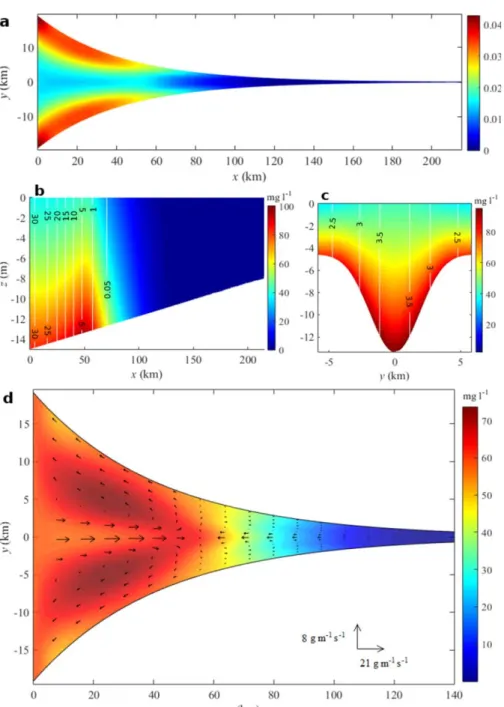
By decreasing the river discharge from 288 to 72 m3s21
, the largest sediment availability moves landward by30 km, and is now located at x130 km (Figure 13a). The residual salt intrusion at Figure 10.Same as (top) Figure 6 and (bottom) Figure 7, but forws50:2 mms21andds510lm.
the central axis of the estuary is enhanced, reaching its landward limit at130 km up-estuary from the mouth, where the maximum residual suspended sediment concentration is found (Figure 13b). At the cross section at x5130 km, salinities are larger in the deeper channel than on the shoals, and the residual sediment concentrations are larger on the shoals than in the middle of the channel (Fig-ure 13c). The depth-integrated residual sediment transport is significantly reduced, with a small sea-ward sediment transport through the deeper channel and landsea-ward transport over the shoals within the ETM region (Figure 13d).
By decreasing the river discharge,TM2 andTM0remain the most dominant sediment transport contributions integrated over the cross section (Figure 14a). The dominance of sediment transport contribution related to the internally generatedM4overtide (TM2IN) becomes more pronounced, and the transport due to the spatial settling lag effects (TSSL
M2) results in a more important landward sediment transport downstream of the ETM Figure 11.Same as Figure 8, but forws51 mms21andds540lm. The cross section in Figure 11c is taken atx5100 km.
and seaward transport upstream of the ETM. The sediment transports due to both river discharge (TRD M0) and gravitational circulation (TGC
M0 andTM2GC) decrease significantly (see Figures 14b and 14c).
Excluding theM2tidal advection of theM2tidal component of concentrations related to the internally
gen-eratedM4tide results in a seaward shift of the ETM from the central estuary to the mouth (see Figure 14a).
By excluding the sediment transport due to the spatial settling lag effects, the ETM slightly shifts toward the Figure 12.Same as (top) Figure 6 and (bottom) Figure 7, but forws51 mms
21
andds540lm.
Table 3
Changes of the Relative Importance of Main Residual Sediment Transport Contributions Integrated Over the Cross Section by Varying Settling Velocities and River Discharges
Transport Decomposition ws50.2 mms21 ws51 mms21 Q572 m3s21 Q5864 m3s21 ds510lm ds540lm TM2 TMGC2 – 1 – 1 TBR M2 – 1 – 1 TIN M2 – 1 1 – TSSL M2 1 1 TM0 TMGC0 1 – 1 TNS M0 – 1 1 – TTRF M0 – 1 1 – TRD M0 1 – – 1
Note. Here ‘‘1’’ and ‘‘2’’ indicate the relative importance of the sediment transport contribution is increased and decreased, respectively, and ‘‘’’ indicates the resulting residual sediment transport changes from a seaward transport contribution to a landward transport contribution, or vice versa.
sea (for less than 10 km), with most sediments trapped in a small region in the central estuary (see Figure 14b). Excluding the gravitational circulation hardly changes longitudinal location of the ETM, but the maxi-mum sediment concentration is reduced (see Figure 14c).
5.2.2. High River Discharge
By increasing the river discharge from 288 to 864 m3s21
, the maximum sediment availability is found near the mouth (Figure 15a). The salt intrusion is dramatically reduced, with the 1 psu isohaline at the central axis of the estuary shifting from125 km to55 km from the mouth (see white lines in Figure 15b). The maximum residual suspended sediment concentration at the central axis of the estuary is found at x50 km (Figure 15b), coinciding the 5 psu isohaline. The residual SSC atx550 km is larger in the deeper channel than on the shoals, and the sediment concentrations become more laterally uniform (Figure 15c). Within the ETM region (x<60 km), sediments are transported landward through the deeper channel, later-ally transporting toward the flanks, and subsequently transported seaward over the shoals (see arrows in
Figure 13.Same as Figure 8, but forQ572 m3s21
Figure 15d). Moreover, it is found that the maximum depth-averaged residual concentrations are located in the center of the transport circulation cells.
ForQ5864 m3s21
, the sediment transport contributionsTM2 andTM0 still dominate the cross-sectionally integrated residual sediment balance (Figure 16a). The major changes in this balance are that, the sediment transport contributions due toM2tidal advection of theM2tidal concentrations related to the internally
generatedM4overtide (TM2IN) decreases and that related to the spatial settling lag effects (TM2SSL) increases. The
landward sediment transport contributions induced by gravitational circulation (TGC
M2 andTM0GC) are also increased. As a result, excluding the sediment transport related to any of these three contributions results in an ETM at the mouth (see Figures 16d–16f).
The main changes of the relative importance of residual sediment transport contributions by varying river discharge are also summarized in Table 3. By decreasing (increasing) river discharge, the river-induced residual flow is decreased (increased), and the ebb-dominant bed shear stress becomes less (more) significant. This results in a reduced residual sediment transport contribution due to advection of residual SSC by river-induced flow (TRD
M0) and a reduced residual transport due toM2tidal advection of
theM2tidal concentration as a result of the river-induced ebb-dominant bed shear stress (included in
TBR
M2). Moreover, decreasing (increasing) river discharge results in smaller (larger) longitudinal and lateral salinity gradients, hence decreasing (increasing) the residual sediment transport contributions related to gravi-tational circulation (TGC
M2;TM0GC), see Table 3. Decreasing (increasing) river discharge also results in narrower (wider) ETM region, which results in a more (less) important residual sediment transport contribution due to spatial settling lag effects (TSSL
M2). The residual sediment transport contributions due to other mechanisms (TIN
M2;TM0TRF) become more (less) dominant, maintaining the balance of the residual sediment transport over the cross section for equilibrium.
6. Model Limitations
6.1. Deviations From Observations
This model requires the net sediment transport through both the seaward and landward boundaries to van-ish, so that the total amount of sediment in the estuary remains unchanged and the condition of morpho-dynamic equilibrium is satisfied. In real estuaries, however, the net sediment transport from the mouth and the landward end may not cancel each other (depending on the strength of tide/wind forcing, river flow, and the sediment availabilities in the adjacent ocean and upper rivers). This would result in a nonequilib-rium state with pointwise deposition/erosion in the estuary and a temporally varying sediment availability distribution. The sediment transport processes in these cases can thus differ significantly from those in equilibrium.
Figure 15.Same as Figure 8, but forQ5864 m3s21