Reduced Life Expectancy Model for Effects of Long Term Exposure on Lethal Toxicity with Fish

(1)

Volume 2013, Article ID 230763,10pages http://dx.doi.org/10.1155/2013/230763

Research Article

Reduced Life Expectancy Model for Effects of Long Term

Exposure on Lethal Toxicity with Fish

Vibha Verma,

1

Qiming J. Yu,

1

and Des W. Connell

2

1_{Griffith School of Engineering, Griffith University, Nathan Campus, Brisbane, Queensland 4111, Australia} 2_{Griffith School of Environment, Griffith University, Nathan Campus, Brisbane, Queensland 4111, Australia}

Correspondence should be addressed to Vibha Verma; [email protected] Received 29 August 2013; Accepted 29 October 2013

Academic Editors: M. Pacheco and S. M. Waliszewski

Copyright © 2013 Vibha Verma et al. This is an open access article distributed under the Creative Commons Attribution License, which permits unrestricted use, distribution, and reproduction in any medium, provided the original work is properly cited. A model based on the concept of reduction in life expectancy (RLE model) as a result of long term exposure to toxicant has been developed which has normal life expectancy (NLT) as a fixed limiting point for a species. The model is based on the equation (LC₅₀= aln(LT₅₀) +b) whereaandbare constants. It was evaluated by plotting ln LT₅₀against LC₅₀with data on organic toxicants obtained from the scientific literature. Linear relationships between LC₅₀and ln LT₅₀were obtained and a Calculated NLT was derived from the plots. The Calculated NLT obtained was in good agreement with the Reported NLT obtained from the literature. Estimation of toxicity at any exposure time and concentration is possible using the model. The use of NLT as a reference point is important since it provides a data point independent of the toxicity data set and limits the data to the range where toxicity occurs. This novel approach, which represents a departure from Haber’s rule, can be used to estimate long term toxicity from limited available acute toxicity data for fish exposed to organic biocides.

1. Introduction

Toxicity is a function of both exposure time period and concentration or dose [1–4]. Nevertheless most of the tox-icological data are based on the quantitative relationship between concentration or dose and adverse effect without consideration of the exposure time period [5–7]. Often imprecise terms such as acute, subacute, subchronic, and chronic are used to describe the exposure time [8]. It is not common to evaluate time as a quantifiable variable of toxicity and often the conditions of toxicity testing are not constant so time cannot be effectively quantified [9].

However there have been studies where exposure time has been evaluated as a quantifiable variable of toxicity [7, 10–12] and the relationship between exposure time and dose has been evaluated [6,13–16]. But in these studies the exposure time is relatively short. While studies based on longer exposure time are important, particularly in the field of risk assessment with environmental contaminants where the exposure time is relatively long and the exposure level is often

low. Information regarding the long term effects of exposure time with environmental chemicals is scarce [17].

The significance of exposure time in toxicological eval-uations was first recognised by Warren [18] describing a relationship((𝐶 − 𝐶₀) × 𝑡 = 𝑘)between exposure time (𝑡) and exposure concentration as the lethal dose to 50% of organisms (𝐶). In this equation𝐶₀is a threshold concentration below which no apparent toxic effects are observed and 𝑘 is a constant. But Haber [19] described it using the simplest form of the relationship between lethal concentration (or dose) and time as(𝐶 × 𝑡 = 𝑘). This relationship was later described as Haber’s rule of inhalation toxicology. Conventionally Haber’s rule, or its modified forms, is used for empirical evaluation of the effect of exposure time on toxicity. To expand the relationship and its application, different variants have been proposed by various researchers [20–22].

However some researchers have noted that the product of(𝐶 × 𝑡)is not always constant [23] especially in the situ-ation when exposure concentrsitu-ation is relatively low and/or exposure time is relatively long [24–26]. According to Haber’s

(2)

rule when the lethal concentration approximates zero, the exposure time must approximate infinity in order to maintain the product as a constant but this is not possible.

A reduced life expectancy (RLE) model has been pro-posed to study the effects of long term exposure [3,27,28]. According to this concept relatively long exposure times at low concentrations of toxicant cause reduction in the normal life expectancy (NLT) of the organism exposed. This model is based on a linear relationship of internal lethal concentration (ILC₅₀) with the natural log of the exposure time with the normal life expectancy (NLT) as a limiting point. Unlike Haber’s rule when the exposure concentration is zero, the exposure time is not infinite but the normal life expectancy of a particular organism.

The RLE model has been evaluated with zooplanktons using data from the scientific literature by plotting ln LT₅₀ (exposure time for 50% lethality of the organisms) against LC₅₀(lethal concentration to 50% of organisms) in ambient water (Verma et al., 2012) [29]. The RLE model successfully fitted most of the zooplanktons data sets; however some sets of data were best fitted by a two-stage version of the RLE model [29]. The concept of reduction in life expectancy has also been used as a measure of toxicity by Mangas-Ram´ırez et al. [30] who studied the effect of cadmium on zooplank-ton. Gama-Flores et al. [31] observed a reduction in life expectancy due to exposure to cadmium with zooplankton.

The objective of this paper was to use life expectancy in the evaluation of the relationship between exposure time and exposure concentration utilising the fish toxicity data available in the scientific literature especially in the situation when exposure time is relatively long.

2. Theory

2.1. Reduced Life Expectancy Model. The RLE model pro-posed by Yu et al. [28] is based on a linear relationship between Internal Lethal Concentration (ILC₅₀) and the nat-ural logarithm of the corresponding exposure time (LT₅₀). The ILC₅₀ is preferred as it is the concentration of toxicant in the organism body at the target site [32–34]. Also it has the advantage that the kinetics effects of the uptake and bioconcentration processes have already been taken into account [3]. The relationship between ILC₅₀ and LT₅₀ for toxicants can be described by the following equation:

ILC₅₀= [ln(NLT) −ln(LT50)]

𝑑 , (1)

where ILC₅₀ is the internal lethal concentration resulting in the death of 50% of the organisms exposed for the time LT₅₀, LT₅₀is the exposure time, NLT is the time until 50% of the organisms die without exposure, and𝑑is a constant. Constant

𝑑 is a measure of toxicity and represents the reduction in life expectancy of the organism per unit concentration of the toxicant.

The value of LT₅₀ represents a reduced life expectancy from the normal life expectancy (NLT) of the organism. When ILC₅₀is plotted against the LT₅₀, the regression line can be extended up to the point where ILC₅₀becomes zero

which corresponds to a toxicant free medium at which the organism would be expected to live its normal life expectancy. The model can be used to predict the reduction in life expectancy at different concentrations of toxicant in the environment. This model has already been tested using the data obtained from earlier work [35] and a high level of correlation between ILC₅₀and LT₅₀was observed [28].

However the limited availability of ILC₅₀ data in the scientific literature [36] restricts the evaluation of the RLE model. Therefore the relationship has been extended from the ILC₅₀to the LC₅₀with the proposal that the relationship between LC₅₀and exposure time period (LT₅₀) can be used to estimate the reduction in life expectancy of organisms [3]. The bioconcentration factor (𝐾_𝐵) for aquatic organisms is the ratio between the concentration of toxicant in the organism (𝐶_𝐵) and the concentration in water (𝐶_𝑊) at equilibrium [3]. Thus

𝐾_𝐵= 𝐶𝐵

𝐶𝑊, (2)

𝐶_𝑊𝛼𝐶_𝐵, (3)

where 𝐶_𝑊 is the lethal concentration (LC₅₀) in water and

𝐶_𝐵the corresponding Internal Lethal Concentration (ILC₅₀). Thus,

LC₅₀𝛼ILC₅₀. (4)

The relationship obtained after replacing ILC₅₀with LC₅₀ in (1) is given as follows: LC₅₀= [ln(NLT) −ln(LT50)] 𝑑 , (5) or LC₅₀= 𝑎ln(LT₅₀) + 𝑏, (6) where𝑎is−1/𝑑and𝑏is ln(NLT)/𝑑.

When LC₅₀is zero, the organism would have a normal life expectancy; thus

LT₅₀ =NLT, (7)

ln(NLT) = 𝑏

𝑎. (8)

According to this model, at LC₅₀ zero (toxicant free environment) organisms would be expected to live to their normal life expectancy. Therefore the model can be used to predict the reduction in the life expectancy at different concentrations of a toxicant in the external environment.

3. Methodology

3.1. Organisms and Toxicants Used for Evaluation. Fish were selected as study organisms since a large volume of toxicity data related to fish are available in the literature. The routes of toxicant uptake common to all fish are through gills, outer body surface, and food. The organic toxicants used in this study were those which had significantly different modes of toxic action and included various organic compounds including organophosphates, organochlorines, pyrethroids, and antiparasites.

(3)

3.2. Sources and Collection of Data. Toxicity data related to fish and organic toxicants were obtained from an extensive search of the literature. The data sets were used which included records of LC₅₀at various exposure durations. Most of the data sets had 4 points where the LC₅₀ had been recorded at 24, 48, 72, and 96 hrs (Table 1) and only the 4 data sets on benzyl compounds withPoecilia reticulatahad more than 4 points with exposure time longer than 96 hrs. The data sets in which LC₅₀required to cause toxicity did not change with exposure time were not processed. Various units for concentration were recorded such as mg/L, g/L, ppm, and ppb, so for consistency all units were converted into𝜇g/L. Similarly the exposure times were also expressed in various units (hours, minutes, and seconds), so all were converted intoday. The Reported NLT data for each organism was also obtained from the literature. When ranges of NLT values were given, the average was calculated to obtain the Reported NLT. The temperature of ambient water used in the experiments ranged between 14∘C and 30∘C.

3.3. Processing of Data. The data sets available for each species of fish were used to evaluate the relationship between LC₅₀and ln(LT₅₀) with the RLE Model as expressed in (6). The LC₅₀ (𝜇g/L) was plotted against ln(LT₅₀) and linear regression analysis was used to obtain the regression equation and correlation coefficient (𝑅2) using Excel. The regression line obtained was extended to the point where the LC₅₀ became zero which corresponded to a toxicant free medium at which the organism would be expected to live its full NLT. The values of the slope (a) and intercept (b) were obtained from the regression equations. These values were then used to obtain the Calculated NLT of each species using (8). The characteristics resulting from this analysis are shown in

Table 1. Only those data which had a minimum of four or more datasets available for each toxicant per fish species were considered to obtain the Calculated NLT (Table 1).

4. Results and Discussion

4.1. Model Evaluation

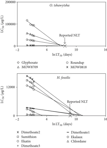
4.1.1. Relationship between Exposure Time and Toxicity. The relationship of toxicity with exposure time was linear and had a negative slope in all cases; examples of the plots are shown inFigure 1. Characteristics of all plots of fish data are listed inTable 1. When𝑅2 was below 0.8, the relationship was not considered to follow a linear trend but only 3 datasets out of 67 were in this category. There are a variety of organic compounds (organophosphates, organochlorines, pyrethroids, and antiparasites) with different mechanisms of action but the relationship of LC₅₀ and ln LT₅₀ was linear with all toxicants. All plots irrespective of toxicant type had negative slopes indicating that lethal toxicity is related to exposure time and LC₅₀required to cause toxicity decreases consistently in a systematic pattern.

4.1.2. The Use of the NLT as Reference Point and as a Limiting Point. According to Haber’s rule (𝐶 × 𝑡 = 𝑘)

0 12000 4 10 16 Dimethoate2 Sumithion Ekatin Dimethoate3 Dimethoate1 Ekalaux Chlordane Reported NLT Reported NLT 0 100000 200000 Glyphosate MOW8709 Roundup MOW0818 H. fossilis O. tshawytsha −2 4 10 16 −2 LC 50 ( 𝜇 g/L) LC 50 ( 𝜇 g/L) ln LT₅₀(days) ln LT₅₀(days)

Figure 1: Examples of plots of LC₅₀against ln LT₅₀with the linear regression line and Reported NLT on the𝑥-axis (Table 1).

when the toxicant concentration is zero, the exposure time is infinity. But according to the RLE model, the NLT is a limiting reference point and when LC₅₀ approximates zero, the exposure time (ln LT₅₀) should be the organism’s normal life expectancy (NLT). Thus maximum possible exposure time of any toxicant to any fish would be the NLT of that particular fish species. The use of NLT as a reference point is important since it limits the maximum exposure time from being infinity at zero exposure concentration (Haber’s rule) to the NLT of the test organism (Figure 1).

4.2. Comparison of the Reported NLT with the Calculated NLT.

The Calculated NLT for each fish species was obtained by the application of characteristics of the relationship obtained from regression analysis of data (Table 1) with (8). The Reported NLT ranging from 360 to 4700 days was plotted against the average Calculated NLT ranging from 120 to 8300 days for various fish species (Figure 2) giving a regression equation as follows:

Reported NLT= 0.996Calculated NLT, 𝑅2= 0.491. (9) There are several sources of error in carrying out a comparison of the Reported NLT with that calculated from

(4)

T a ble 1: R egr essio n anal ysis o f the re la ti o n shi p b etw een lnL T50 an d LT 50 . Fish sp ecies: o rga nic co m p o u nds Rep o rt ed NL T da y (lnNL T ) Cal cul at ed N LT da y (lnNL T ) ∗∗ In te rcep t ( 𝑏 )S lo p e ( 𝑎 ) ∗ Reg ressio n co efficien t ( 𝑅 2 ) R ef er ence Or eo ch ro m is n il ot ic us Dimet h o at e 50 0 (6.22) (M ug isha an d D d u m b a, 20 0 6 [ 37 ]) 4 80 (6.18) 36 ,000 − 7, 80 0 0 .9 49 P h o m m ak o n e,2 0 0 4[ 38 ] Dimet h o at e 34 ,000 − 3,4 0 0 0.9 0 0 Ca p ta n 580 − 13 0 0.98 4 B o ra n et al ., 2012 [ 39 ] 2,3,4,5-T et rac h lo ro p h eno l 31 0 − 58 0.6 27 H o lco m b e et al ., 19 84 [ 40 ] On co rh yn ch us go rb usc h a Glyphos ate 6 0 0 (6.3 9) (H ea le y, 19 86 [ 41 ]; Sc o tt and Cr os sma n ,1 97 3 [ 42 ]) 120 (4.7 8) 13 0 ,000 − 50,0 0 0 0.9 62 W an et al ., 198 9 [ 43 ] MO W 0 818 3,3 0 0 − 6 4 0 0.98 5 MO W 870 9 60 ,000 − 21,0 0 0 0.94 3 R o u n dup 28 ,000 − 3,0 0 0 0.957 Sa lm o ga ir d n eri 2,3,4,5-T et rac h lo ro p h eno l 33 0 0 (8.1) (G o rbac h ,1 9 61 [ 44 ]) 54 0 0 (8.6) 10 0 ,000 − 9, 4 0 0 0.8 32 H o lco m b e et al ., 19 84 [ 40 ] Glyphos ate 2, 600 − 36 0 0.97 7 W an et al ., 19 89 [ 43 ] MW08 18 4 5, 000 − 10,0 0 0 0.986 MO W 870 9 22 ,000 − 1,80 0 0.98 2 R o u n dup On co rh yn ch us ts h awy te sh a Glyphos ate 21 0 0 (7 .6 5) (M o yle ,2 0 02 [ 45 ]; H eale y [ 41 ]) 20 0 0 (7 .6 0) 11 0 ,000 − 17 ,0 0 0 0.88 5 W an et al ., 19 89 [ 43 ] MW08 18 3, 000 − 36 0 0.9 05 MO W 870 9 58 ,000 − 7, 9 0 0 0.98 4 R o u n dup 29 ,000 − 3,6 0 0 0.97 8 On co rh yn ch us ke ta Glyphos ate 27 0 0 (7 .8) (S co tt an d C ro ssma n, 19 73 [ 42 ]) 38 0 0 (8.2 3) 89 ,000 − 14,0 0 0 0.9 98 W an et al ., 198 9 [ 43 ] MO W 0 818 2,4 0 0 − 19 0 0.8 18 MO W 870 9 44 ,000 − 4,9 0 0 0.95 6 R o u n dup 23 ,000 − 4,4 0 0 0.980 On co rh yn ch us ki su tc h Glyphos ate 18 0 0 (7 .5 1) (S co tt an d C ro ssma n, 19 73 [ 42 ]) 26 0 0 (7 .88) 12 ,000 − 2,0 0 0 0.98 4 W an et al ., 19 89 [ 43 ] MO W 0 818 3,3 0 0 − 31 0 0.8 20 MO W 870 9 4 8, 000 − 5,20 0 0.8 23 R o u n dup 34 ,000 − 5,10 0 0.97 2 A n gu il la an gu il la M et h yl pa ra thio n 47 0 0 (8.4 6) (EC F isher ies, 2013 [ 46 ]) 37 0 0 (8.22) 54,0 0 − 87 0 0.97 7 F er ra ndo et al ., 19 91 [ 47 ] M et h ilda thio n 3,7 0 0 − 1,7 0 0 0.9 67 C h lo rp yr if os 1,20 0 − 55 0 0.9 05 T ric hlo rf o n 4,9 0 0 − 1,20 0 0.9 30 F eni tr o thio n 340 − 13 0 0.8 17 Endosulfa n 52 − 1.3 0.7 4 2 Diazino n 16 0 − 59 0.981

(5)

Ta b le 1: C o n ti n u ed . Fish sp ecies: o rga nic co m p o u nds Rep o rt ed NL T da y (lnNL T ) Cal cul at ed N LT da y (lnNL T ) ∗∗ In te rcep t ( 𝑏 )S lo p e ( 𝑎 ) ∗ Reg ressio n co efficien t ( 𝑅 2 ) R ef er ence H et er op en te u s( Sa cc ob ra n ch u s)f os si li s Dimet h o at e 6 6 0 0 (8.79) (Flo w er ,1 92 5 [ 48 ]; Al tma n an d D itt m er ,1 9 62 [ 49 ]) 810 0 (9 .0 2) 17 ,000 − 1, 600 0 .9 30 Dimet h o at e 3,4 0 0 − 30 0 0.9 6 6 P ande y et al ., 20 0 9 [ 50 ] Dimet h o at e 3,4 0 0 − 29 0 0.98 2 Chl o rd an e 500 − 86 0.9 92 P ande y et al ., 20 08 [ 51 ] Ek at in 13 ,000 − 1,10 0 0.9 29 V er m a et al ., 197 8 [ 52 ] Ek ala u x 2,80 0 − 9 0 0 0.94 3 Sumi thio n 15 ,000 − 1, 600 0 .8 71 P oecil ia.r eticula ta Me th yl b en zo at e 55 0 (6.3) (Fish B as e [ 53 ]) 220 (5.4) Be n zo n it ri le 59 ,000 − 12,0 0 0 0.9 31 V erhaa r et al ., 19 9 9 [ 54 ] B enzaldeh yde 24 0 ,000 − 4 2,0 0 0 0.9 08 B enzy lalco ho l 23 ,000 − 6,20 0 0.8 30 C yp er m et hr in 640 ,000 − 210,0 0 0 0.9 11 C yp er m et hr in 3,20 0 − 67 0 0.97 8 G au ta ra an d G u p ta ,2 0 0 8 [ 55 ] C yp er m et hr in 2,20 0 − 36 0 0.95 6 C yp er m et hr in 1,9 0 0 − 28 0 0.9 91 C yp er m et hr in 1,80 0 − 210 0.9 62 C yp er m et hr in 2,5 0 0 − 52 0 0.97 8 C yp er m et hr in 2,4 0 0 − 4 6 0 0.98 3 P ime phal es pr ome la s 2-A lly lp henol 72 0 (6.58) (S co tt an d Cr os sma n 19 73 [ 42 ]) 73 0 (6.5 9) 32 ,000 − 15,0 0 0 0.9 15 H o lco m b e et al ., 19 84 [ 40 ] 4 -T er t-b ut yl phe n ol 6,20 0 − 80 0 0.98 9 4-C h lo ro -3-met h yl p heno l 14,0 0 0 − 4,10 0 0.9 6 6 4-N it ro p henol 65 ,000 − 18,0 0 0 0.98 5 2,3,4,5-T et ra p h en yl 49 0 − 4 0 0.88 2 1,4-Dini tr ob enzene 69 0 − 6 0 0.98 2 Ic talutr u s punc ta tu s 1,4-Dini tr ob enzene 29 0 0 (8.3 0) (J ea rld and B ro w n, 19 71 [ 56 ]) N/A ∗∗∗ 910 − 17 0 0.97 1 H o lco m b e et al ., 198 4 [ 40 ] 2-E tho x yet h yl lacet at e 21 ,000 − 4,20 0 0.94 6 C h an na pu nc ta tu s Ca rb o sul fa n 20 0 0 (7 .6 0) (N ay ak et al ., 1999 [ 57 ]) N/A ∗∗∗ 1, 600 − 1, 0 0 0 0 .8 30 N w an ie ta l.,2 01 0[ 58 ] Glyphos ate 41,0 0 0 − 7, 4 0 0 0.7 69 A trazine 63 ,000 − 16,0 0 0 0.958 Cy pr in u s ca rp io Dic h lo rv os 17 16 0 (9 .7 5) (Flo w er ,1 92 5 [ 48 ]) N/A ∗∗∗ 37 ,000 − 1,10 0 0.9 32 D as, 2012 [ 59 ] Dimet h o at e 1,9 0 0 − 16 0 0 .9 36 Si n ghe ta l.,2 0 0 9[ 60 ] T ric hogas ter tr ic ho pt er u s Diazino n 15 0 0 (7 .3 1) N/A ∗∗∗ 40 ,000 − 18,0 0 0 0.98 9 D el ta m et hr in 300 − 53 0.8 9 0 H eda ya ti et al ., 2012 [ 61 ]

(6)

Ta b le 1: C o n ti n u ed . Fish sp ecies: o rga nic co m p o u nds Rep o rt ed NL T da y (lnNL T ) Cal cul at ed N LT da y (lnNL T ) ∗∗ In te rcep t ( 𝑏 )S lo p e ( 𝑎 ) ∗ Reg ressio n co efficien t ( 𝑅 2 ) R ef er ence On co rh yn ch us m yk is s m-Cr es o l 1,3 0 0 (S co tt an d C ro ssma n, 19 73 [ 42 ]) N/A ∗∗∗ 8, 000 − 3, 000 0 .999 Ca p k in et al ., 20 10 [ 62 ] D el ta m et hr in 4.5 − 3.4 0.98 2 U ral and Sa ˘gla m ,2 0 0 5 [ 63 ] Endosulfa n 19 − 13 0.987 C ap kin et al ., 20 0 6 [ 64 ] Ga m bus ia affi n is m-Cr es o l 70 0 (K ru mho lz, 19 4 8 [ 65 ]) N/A ∗∗∗ 40 ,000 − 5, 600 0 .8 94 Sa n gl i an d K an ab u r, 2000 [ 66 ] ∗LC 50 = 𝑎 lnL T50 + 𝑏 , ∗∗calc ula ted fr o m ln NL T50 = −𝑏 / 𝑎 ,( 8 ), ∗∗∗ th es e sp ecies had < 4d at as et s.

(7)

5 8 11 5 8 11 Reported NLT=0.9975 Calculated NLT = 0.4923 R2 Rep o rt ed (ln LT 50 ) Calculated (ln NLT₅₀)

Figure 2: Plot of the Calculated NLT with the Reported NLT with linear regression line (Table 1).

the RLE Model. An important factor is the decision on death during the toxicity test with fish considered dead becoming mobile when transferred to toxicant free water [67]. In addition there are many discrepancies regarding the Reported NLT. For example, Mugisha and Ddumba [37] reported the life expectancy of O. niloticus as 1 to 1.5 yrs, while Ofori-Danson and Kwarfo-Apegyah [68] have reported the life expectancy as 5 yrs. Changes in the temperature of ambient water affects fish life expectancy [69]. In warmer water the fish generally grows faster but the lifespan becomes shorter than in a cold environment [70]. Thus mortality can be related to growth and temperature [71]. It can be also expected that NLT would vary depending on such factors as oxygen availability, food, and so on. It is noteworthy that there are reports that the same fish species can have different life expectancies in different parts of the world [72–75].

Even though there are possible reasons for the Calculated NLT to differ from the Reported NLT as outlined above but overall the Reported NLT and Calculated NLT are in reasonably good agreement.

4.3. Application of the RLE Model

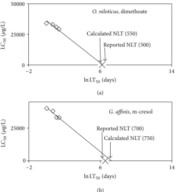
4.3.1. Toxicity at Longer Exposures Times. The novel approach of the RLE model (6) allows the acute toxicity data available in the literature to be used for estimation of LC₅₀ at other exposure times and also chronic toxicity. The equations obtained from regression analysis of LC₅₀ versus ln LT₅₀ (Table 1) can be used to estimate toxicity at any exposure time and exposure concentration for a particular fish species. For example plots of the LC₅₀versus ln LT₅₀using acute toxicity data of the toxicants dimethoate and m-cresol with the fish speciesO. niloticusandG. affinisare shown in Figures3(a) and3(b), respectively. It should be noted that the regression line intersects with the 𝑥-axis close to the Reported NLT (Figure 3) in both species. The regression equations obtained from this analysis are as described as follows:

𝑂. 𝑛𝑖𝑙𝑜𝑡𝑖𝑐𝑢𝑠 LC₅₀= −5800ln LT₅₀+ 36000 𝑅2= 0.971, (10) 0 25000 6 14 Calculated NLT (750) 0 25000 50000 Reported NLT (500) Calculated NLT (550) −2 6 14 −2 O. niloticus, dimethoate G. affinis, m-cresol Reported NLT (700) LC 50 ( 𝜇 g/L) LC 50 ( 𝜇 g/L) ln LT₅₀(days) ln LT₅₀(days) (a) (b)

Figure 3: Example of plots of LC₅₀versus ln LT₅₀using the RLE model for estimation of long term toxicity.

𝐺. 𝑎𝑓𝑓𝑖𝑛𝑖𝑠 LC₅₀= −1600ln LT₅₀+ 15000 𝑅2= 0.894. (11) Using (10), where the slope (𝑎) is−5800 and the intercept (𝑏) is 36000, the LC₅₀ of dimethoate with fishO. niloticus

at any exposure time (ln LT₅₀) can be calculated. Similarly using (11), the toxicity, as LC₅₀of m-cresol toG. affinisat any exposure time (ln LT₅₀) can be obtained.

After plotting the toxicity data (LC₅₀ versus lnLT₅₀) obtained from the literature for a particular toxicant and fish species, application of (6) will give an estimate of toxicity of that particular toxicant for any exposure time particularly long ones.

When the toxicity information available is in the form of only one endpoint, most commonly the 96 hrs LC₅₀, an estimation of toxicity at other exposure times is possible. This is done by using NLT of a particular organism as a limiting reference point. Firstly the LC₅₀versus ln LT₅₀can be plotted by using the 96 hr endpoint data from the literature, as one data point and the Reported NLT of the particular fish species as the second data point and an equation can be obtained from analysis of this relationship. This approach can be used to estimate toxicity at any exposure time, including long times for a particular fish species.

4.3.2. Estimation of Normal Life Expectancy (NLT). This approach can also be used to estimate the approximate NLT of a fish species. For the estimation of NLT, the first step is to plot LC₅₀versus ln LT₅₀recorded at various exposure times of as many data sets as possible related to that particular fish species. After calculation of the ln NLT₅₀by the use of (8)

(8)

then the average of these individual NLT can be obtained, which is the average Calculated NLT for that particular fish species.

5. Conclusions

The relationship of toxicity with exposure time for fish using the equation given below was linear in almost all cases, had a negative slope, and is expressed as

LC₅₀= 𝑎ln(LT₅₀) + 𝑏. (12) This equation with parameters derived empirically for a particular fish species can be used to estimate toxicity at any exposure time particularly long exposure times.

The use of NLT as a limiting reference point is innovative since it limits the data to the range where toxicity occurs. In addition it provides a reference point which is independent from the toxicity data set, when the toxicant concentration is zero the life span is the normal life expectancy of the fish species. The equation above then becomes ln NLT = 𝑏/𝑎. This is in contrast to Haber’s rule from which an exposure time of infinity is obtained when the exposure concentration is zero.

In support of the relationship above the Calculated NLT and Reported NLT were in good agreement as expressed by the following relationship:

Reported NLT= 0.998Calculated NLT, 𝑅2= 0.4923. (13) Available acute toxicity data can be used to calculate toxicity for a particular fish species exposed to organic biocides at any exposure time. Even with limited information (endpoint only) available the lethal toxicity estimation at any exposure is possible.

References

[1] J. Baas, T. Jager, and B. Kooijman, “Understanding toxicity as processes in time,”Science of the Total Environment, vol. 408, no. 18, pp. 3735–3739, 2010.

[2] V. Bonnomet, C. Duboudin, H. Magaud, E. Thybaud, E. Vin-dimian, and B. Beauzamy, “Modeling explicitly and mechanis-tically median lethal concentration as a function of time for risk assessment,”Environmental Toxicology and Chemistry, vol. 21, no. 10, pp. 2252–2259, 2002.

[3] D. Connell and J. Yu, “Use of exposure time and life expectancy in models for toxicity to aquatic organisms,”Marine Pollution Bulletin, vol. 57, no. 6-12, pp. 245–249, 2008.

[4] L. S. McCarty, P. F. Landrum, S. N. Luoma et al., “Advancing environmental toxicology through chemical dosimetry: exter-nal exposures versus tissue residues,”Integrated Environmental Assessment and Management, vol. 7, no. 1, pp. 7–27, 2011. [5] R. Ashauer and B. I. Escher, “Advantages of toxicokinetic and

toxicodynamic modelling in aquatic ecotoxicology and risk assessment,”Journal of Environmental Monitoring, vol. 12, no. 11, pp. 2056–2061, 2010.

[6] T. Jager and S. A. L. M. Kooijman, “A biology-based approach for quantitative structure-activity relationships (QSARs) in ecotoxicity,”Ecotoxicology, vol. 18, no. 2, pp. 187–196, 2009.

[7] F. S´anchez-Bayo, “From simple toxicological models to predic-tion of toxic effects in time,”Ecotoxicology, vol. 18, no. 3, pp. 343– 354, 2009.

[8] K. K. Rozman and J. Doull, “Dose and time as variables of toxicity,”Toxicology, vol. 144, no. 1–3, pp. 169–178, 2000. [9] K. K. Rozman and J. Doull, “The role of time as a

quan-tifiable variable of toxicity and the experimental conditions when Haber’s c x t product can be observed: implications for therapeutics,”Journal of Pharmacology and Experimental Therapeutics, vol. 296, no. 3, pp. 663–668, 2001.

[10] M. A. Beketov and M. Liess, “Acute and delayed effects of the neonicotinoid insecticide thiacloprid on seven freshwater arthropods,”Environmental Toxicology and Chemistry, vol. 27, no. 2, pp. 461–470, 2008.

[11] T. Jager, T. Vandenbrouck, J. Baas, W. M. De Coen, and S. A. L. M. Kooijman, “A biology-based approach for mixture toxicity of multiple endpoints over the life cycle,”Ecotoxicology, vol. 19, no. 2, pp. 351–361, 2010.

[12] T. Jager and E. I. Zimmer, “Simplified dynamic energy budget model for analysing ecotoxicity data,”Ecological Modelling, vol. 225, pp. 74–81, 2012.

[13] O. A. ´Alvarez, T. Jager, B. N. Colao, and J. E. Kammenga, “Temporal dynamics of effect concentrations,”Environmental Science and Technology, vol. 40, no. 7, pp. 2478–2484, 2006. [14] M. C. Newman and M. S. Aplin, “Enhancing toxicity data

interpretation and prediction of ecological risk with survival time modeling: an illustration using sodium chloride toxicity to mosquitofish (Gambusia holbrooki),”Aquatic Toxicology, vol. 23, no. 2, pp. 85–96, 1992.

[15] D. Pascoe and N. A. M. Shazili, “Episodic pollution—a com-parison of brief and continuous exposure of rainbow trout to cadmium,”Ecotoxicology and Environmental Safety, vol. 12, no. 3, pp. 189–198, 1986.

[16] K. K. Rozman, “Quantitative definition of toxicity: a mathemati-cal description of life and death with dose and time as variables,” Medical Hypotheses, vol. 51, no. 2, pp. 175–178, 1998.

[17] T. Jager and C. Klok, “Extrapolating toxic effects on individuals to the population level: the role of dynamic energy budgets,” Philosophical Transactions of the Royal Society B, vol. 365, no. 1557, pp. 3531–3540, 2010.

[18] E. Warren, “On the reaction of Daphnia magna (straus) to certain changes in its environment,”Quarterly Journal of Micro-scopical Science, vol. 43, pp. 199–224, 1900.

[19] F. Haber, “On the history of gas warfare,” inFive Lectures from the Years 1920–1923, pp. 75–92, Springer, Berlin, Germany, 1924, (German).

[20] A. J. Clark, “General pharmacology,” inHandbuch der Experi-mentellen Pharmakologie, W. Heubner and J. Schuller, Eds., vol. 4, pp. 123–142, Springer, Berlin, Germany, 1937.

[21] C. I. Bliss, “The relation between exposure time, concentration and toxicity in experiments on insecticide,” Annals of the Entomological Society of America, vol. 33, pp. 721–766, 1940. [22] H. Druckrey and K. Kupfmuller, “Quantitative analysis of

carcinogenesis,”Zeitschrift f¨ur Naturforschung B, vol. 3, pp. 254– 266, 1948 (German).

[23] F. Flury and W. Wirth, “Toxicology of the solvents (various esters, acetone, methyl alcohol),”Archiv f¨ur Gewerbepathologie und Gewerbehygiene, vol. 5, pp. 2–90, 1934 (German). [24] D. E. Gardner, F. J. Miller, E. J. Blommer, and D. L. Coffin,

“Influ-ence of exposure mode on the toxicity of NO₂,”Environmental Health Perspectives, vol. 30, pp. 23–29, 1979.

(9)

[25] E. Weller, N. Long, A. Smith et al., “Dose-rate effects of ethy-lene oxide exposure on developmental toxicity,”Toxicological Sciences, vol. 50, no. 2, pp. 259–270, 1999.

[26] S. Yoshimura, K. Imai, Y. Saitoh, H. Yamaguchi, and S. Ohtaki, “The same chemicals induce different neurotoxicity when administered in high doses for short term or low doses for long term to rats and dogs,”Molecular and Chemical Neuropathology, vol. 16, no. 1-2, pp. 59–84, 1992.

[27] Y. Chaisuksant, Q. Yu, and D. Connell, “Internal lethal concen-trations of halobenzenes with fish (Gambusia affinis),” Ecotoxi-cology and Environmental Safety, vol. 37, no. 1, pp. 66–75, 1997. [28] Q. Yu, Y. Chaisuksant, and D. Connell, “A model for

non-specific toxicity with aquatic organisms over relatively long periods of exposure time,”Chemosphere, vol. 38, no. 4, pp. 909– 918, 1999.

[29] V. Verma, J. Yu, and D. W. Connell, “Evaluation of effects of exposure time on aquatic toxicity with zooplanktons using a reduced life expectancy model,”Chemosphere, vol. 89, pp. 1026– 1033, 2012.

[30] E. Mangas-Ram´ırez, S. S. S. Sarma, and S. Nandini, “Recovery patterns of Moina macrocopa exposed previously to different concentrations of cadmium and methyl parathion: life-table demography and population growth studies,”Hydrobiologia, vol. 526, no. 1, pp. 255–265, 2004.

[31] J. L. Gama-Flores, S. S. S. Sarma, and S. Nandini, “Exposure time-dependent cadmium toxicity toMoina macrocopa (Clado-cera): a life table demographic study,”Aquatic Ecology, vol. 41, no. 4, pp. 639–648, 2007.

[32] R. Ashauer, A. B. A. Boxall, and C. D. Brown, “Predicting effects on aquatic organisms from fluctuating or pulsed exposure to pesticides,”Environmental Toxicology and Chemistry, vol. 25, pp. 1899–1912, 2006.

[33] D. W. Connell, Y. Chaisuksant, and J. Yu, “Importance of internal biotic concentrations in risk evaluations with aquatic systems,”Marine Pollution Bulletin, vol. 39, no. 1-12, pp. 54–61, 1999.

[34] B. I. Escher, R. Ashauer, S. Dyer et al., “Crucial role of mechanisms and modes of toxic action for understanding tissue residue toxicity and internal effect concentrations of organic chemicals,”Integrated Environmental Assessment and Management, vol. 7, no. 1, pp. 28–49, 2011.

[35] Y. Chaisuksiant, Q. Yu, and D. W. Connell, “The internal critical level concept of nonspecific toxicity,”Reviews of Environmental Contamination and Toxicology, vol. 162, pp. 1–41, 1999. [36] V. Maeder, B. I. Escher, M. Scheringer, and K. Hungerb¨uhler,

“Toxic ratio as an indicator of the intrinsic toxicity in the assess-ment of persistent, bioacculumulative, and toxic chemicals,” Environmental Science and Technology, vol. 38, no. 13, pp. 3659– 3666, 2004.

[37] J. Y. T. Mugisha and H. Ddumba, “On the dynamics of a fisheries model with feeding patterns and harvesting: late niloticus and O. niloticus in Lake Victoria,” in Mathamatical Biology and Biocomplexcity Workshop Africa, University of Capetown, Capetown, South Africa, 2006.

[38] S. Phommakone,The toxic effects of pesticides dimethoate and profenofos on nile tilapia fry (Oreochromis niolticus) and water flea (Moina macrocopa) [Ph.D. thesis], Asian Institute of Tech-nology, School od Environment and Resources Development, Pathumthani, Thailand, 2004.

[39] H. Boran, E. Capkin, I. Altinok, and E. Terzi, “Assessment of acute toxicity and histopathology of the fungicide captan in

rainbow trout,”Experimental and Toxicologic Pathology, vol. 64, no. 3, pp. 175–179, 2012.

[40] G. W. Holcombe, G. L. Phipps, M. L. Knuth, and T. Felhaber, “The acute toxicity of selected substituted phenols, benzenes and benzoic acid esters to fathead minnowsPimephales prome-las,”Environmental Pollution Series A, vol. 35, no. 4, pp. 367–381, 1984.

[41] M. C. Healey,Salmonid Age at Maturity, vol. 89 ofCanadian Special Publication of Fisheries and Aquatic Sciences, Dept. of Fisheries and Oceans, 1986.

[42] W. Scott and E. Crossman, “Freshwater fishes of Canada,” Fisheries Research Board of Canada Bulletin, vol. 184, p. 966, 1973.

[43] M. T. Wan, R. G. Watts, and D. J. Moul, “Effects of different dilution water types on the acute toxicity to juvenile pacific salmonids and rainbow trout of glyphosate and its formulated products,”Bulletin of Environmental Contamination and Toxi-cology, vol. 43, no. 3, pp. 378–385, 1989.

[44] E. J. Gorbach, “Age composition, growth and age of onset of sexual maturity of white Ctenopharyhgodon idella (Val) and bleck Mylopharyngodon pisceus (Rich amur) in the Amur river basin,”Voprosy Ikhtiologii, vol. 1, pp. 119–126, 1961.

[45] B. P. Moyle,Inland Fishes of California, University of California, California Press, 2nd edition, 2002.

[46] EuropeanCommission, “Fisheries: Eel (Anguilla anguilla),”

http://ec.europa.eu/fisheries/marine species/wild species/eel/

index en.htm.

[47] M. D. Ferrando, E. Sancho, and E. Andreu-Moliner, “Compar-ative acute toxicities of selected pesticides toAnguilla anguilla,” Journal of Environmental Science and Health. Part B, vol. 26, no. 5-6, pp. 491–498, 1991.

[48] M. S. S. Flower, “Contributions to our knowledge of the duration of life in vertebrate animals—I. Fishes,”Proccedings of the Zoological Society of London, vol. 1, pp. 247–267, 1925. [49] P. L. Altman and D. S. Dittmer, “Growth including reproduction

and morphological development,” in Biological Handbooks, Federation of American Societies for Experimental Biology, Washington, DC, USA, 1962.

[50] R. K. Pandey, R. N. Singh, S. Singh, N. N. Singh, and V. K. Das, “Acute toxicity bioassay of dimethoate on freshwater airbreathing catfish,Heteropneustes fossilis(Bloch),”Journal of Environmental Biology, vol. 30, no. 3, pp. 437–440, 2009. [51] R. K. Pandey, R. N. Singh, and V. K. Das, “Effect of temperature

on mortality and behavioural responses in freshwater catfish Heteropneustes fossilis(Bloch) exposed to dimethoate,”Global Journal of Environmental Research, vol. 2, no. 3, pp. 126–132, 2008.

[52] S. R. Verma, S. K. Bansal, and R. C. Dalela, “Toxicity of selected organic pesticides to a fresh water teleost fish, Saccobranchus fossilis and its application in controlling water pollution,” Archives of Environmental Contamination and Toxicology, vol. 7, no. 3, pp. 317–323, 1978.

[53] R. Froese and D. Pauly, Eds.,Fish Base, World Wide Web Electronic Publication, 2012,http://www.fishbase.org/. [54] H. J. M. Verhaar, W. de Wolf, S. Dyer, K. C. H. M. Legierse,

W. Seinen, and J. L. M. Hermens, “An LC₅₀ vs time model for the aquatic toxicity of reactive and receptor-mediated compounds. Consequences for bioconcentration kinetics and risk assessment,”Environmental Science and Technology, vol. 33, no. 5, pp. 758–763, 1999.

(10)

[55] P. P. Gautara and A. K. Gupta, “Toxicity of cypermethrin to the juveniles of freshwater fish Poecilia reticulata (Peters) in relation to selected environmental variables,”Natural Product Radiance, vol. 7, no. 4, pp. 314–319, 2008.

[56] A. Jearld Jr. and B. E. Brown, “Fecundity, age and growth and condition of channel catfish in Oklahoma reservoir,” Proceed-ings of the Oklahoma Academy of Science, vol. 51, pp. 15–22, 1971. [57] S. B. Nayak, B. S. Jena, and B. K. Patnaik, “Effects of age and manganese (II) chloride on peroxidase activity of brain and liver of the teleost, Channa punctatus,”Experimental Gerontology, vol. 34, no. 3, pp. 365–374, 1999.

[58] C. D. Nwani, N. S. Nagpure, R. Kumar, B. Kushwaha, P. Kumar, and W. S. Lakra, “Lethal concentration and toxicity stress of carbosulfan, glyphosate and atrazine to freshwater air breathing fishChanna punctatus(Bloch),”International Aquatic Research, vol. 2, pp. 105–111, 2010.

[59] S. Das, “A review of Dichlorvos toxicity in fish,”Current World Environment, 2012.

[60] R. N. Singh, R. K. Pandey, N. N. Singh, and V. K. Das, “Acute toxicity and behavioural response of common carp Cyprinus carpio(Linn) to an organophosphae (dimethoate),” World Journal of Zoology, vol. 4, no. 2, pp. 70–75, 2009. [61] A. Hedayati, T. Reza, and A. Shadi, “Investigation of acute

toxicity of two pesticides diazinon and deltamethrin, on Blue Gourami,Trichogaster trichopterus(Pallus),”Global Veterinaria, vol. 8, no. 5, pp. 440–444, 2012.

[62] E. Capkin, S. Kayis, H. Boran, and I. Altinok, “Acute toxicity of some agriculture fertilizers to rainbow trout,” inTurkish Journal of Fisheries and Aquatic Sciences, vol. 10, pp. 19–25, 2010. [63] M. S¸. Ural and N. Saˇglam, “A study on the acute

toxi-city of pyrethroid deltamethrin on the fry rainbow trout (Oncorhynchus mykissWalbaum, 1792),”Pesticide Biochemistry and Physiology, vol. 83, no. 2-3, pp. 124–131, 2005.

[64] E. Capkin, I. Altinok, and S. Karahan, “Water quality and fish size affect toxicity of endosulfan, an organochlorine pesticide, to rainbow trout,”Chemosphere, vol. 64, no. 10, pp. 1793–1800, 2006.

[65] L. A. Krumholz, “Reproduction in the western mosquitofish, Gambusia affinis affinis (Baird and Girad), and its use in mosquito control,” Ecological Monographs, vol. 18, pp. 1–43, 1948.

[66] A. B. Sangli and V. V. Kanabur, “Acute toxicity of cresol and chlorophenol to a freshwater fishGambusia affinisand their effects on oxygen uptake,”Journal of Environmental Biology, vol. 21, no. 3, pp. 215–217, 2000.

[67] W. L. Chadderton, S. Kelleher, A. Brow, T. Shaw, B. Studholme, and R. Barrier, “Testing the efficacy of rotenone as a piscicide for New Zealand pest fish species,” inManaging Invasive Freshwater Fish in New Zealand. Proceedings of a Workshop, pp. 113–130, Department of Conservation Science Publishing, Hamilton, New Zealand, 2001.

[68] P. K. Ofori-Danson and K. Kwarfo-Apegyah, “An assessment of the cichlid fishery of bontanga reservoir, Northern Ghana,”West African Journal of Applied Ecology, vol. 14, 2009.

[69] P. A. Azevedo, C. Y. Cho, S. Leeson, and D. P. Bureau, “Effects of feeding level and water temperature on growth, nutrient and energy utilization and waste outputs of rainbow trout (Oncorhynchus mykiss),”Aquatic Living Resources, vol. 11, no. 4, pp. 227–238, 1998.

[70] R. L. Beschta, R. E. Bibly, G. W. Brown, L. B. Holtby, and T. D. Hofstra, “Stream temperature and aquatic habitat,” in

Streamside Management: Forestry and Fishery Interactions, E. O. Salo and T. W. Cundy, Eds., Contribution no. 57, pp. 191–232, University of Washington, Institute of Forest Resources, 1987. [71] D. Griffiths and C. Harrod, “Natural mortality, growth

parame-ters, and environmental temperature in fishes revisited,” Cana-dian Journal of Fisheries and Aquatic Sciences, vol. 64, no. 2, pp. 249–255, 2007.

[72] A. Blanck and N. Lamouroux, “Large-scale intraspecific varia-tion in life-history traits of European freshwater fish,”Journal of Biogeography, vol. 34, no. 5, pp. 862–875, 2007.

[73] J.-F. Duchesne and P. Magnan, “The use of climate classification parameters to investigate geographical variations in the life history traits of ectotherms, with special reference to the white sucker (Catostomus commersoni),”Ecoscience, vol. 4, no. 2, pp. 140–150, 1997.

[74] E. Heibo, C. Magnhagen, and L. A. Vøllestad, “Latitudinal variation in life-history traits in Eurasian perch,”Ecology, vol. 86, no. 12, pp. 3377–3386, 2005.

[75] P. Roni and T. P. Quinn, “Geographic variation in size and age of North American chinook salmon,”North American Journal of Fisheries Management, vol. 15, no. 2, pp. 325–345, 1995.

(11)

Submit your manuscripts at

http://www.hindawi.com

Pain

_{Research and Treatment}

Hindawi Publishing Corporation

http://www.hindawi.com Volume 2014

World Journal

Toxins

Journal of

Vaccines

Journal of

Antibiotics

Toxicology

Journal of

Stroke

_{Research and Treatment}

Drug Delivery

Journal of Hindawi Publishing Corporation

http://www.hindawi.com Volume 2014 Hindawi Publishing Corporation

http://www.hindawi.com Volume 2014 Advances in Pharmacological Sciences

Tropical Medicine

Medicinal ChemistryInternational Journal of Hindawi Publishing Corporation

Addiction

Journal of

http://www.hindawi.com Volume 2014 BioMed

Research International Emergency Medicine International

Diseases

Anesthesiology Research and Practice

Scientifica

Journal of

Reduced Life Expectancy Model for Effects of Long Term Exposure on Lethal Toxicity with Fish

Research Article