Generalized Additive Modelling of Mixed Distribution Markov Models with Application to Melbourne's Rainfall.

M O N A S H U N I V E R S I T Y

AUSTRALIA

Generalized Additive Modelling of Mixed Distribution

Markov Models with Application to Melbourne’s Rainfall

Rob J. Hyndman & Gary K. Grunwald

Working Paper 2/99

January 1999

DEPARTMENT OF ECONOMETRICS

AND BUSINESS STATISTICS

Markov models with application to Melbourne’s

rainfall

Rob J. Hyndman1 and Gary K. Grunwald2 11 December 1998

Abstract: We consider modelling time series using a generalized additive model with first-order Markov structure and mixed transition density having a discrete component at zero and a continuous component with positive sample space. Such models have application, for example, in modelling daily occurrence and intensity of rainfall, and in modelling the number and size of insurance claims.

We show how these methods extend the usual sinusoidal seasonal assumption in standard chain-dependent models by assuming a general smooth pattern of occurrence and intensity over time. These models can be fitted using standard statistical software. The methods of Grunwald and Jones (1998) can be used to combine these separate occurrence and intensity models into a single model for amount. We use 36 years of rainfall data from Melbourne, Australia, as a vehicle of illustration, and use the models to investigate the effect of the El

Ni˜no phenomenon on Melbourne’s rainfall.

1 Introduction

Time series with a mixed density composed of a discrete component at zero and a continuous component on the positive real line commonly occur with meteorological and environmen-tal data where there may be no recordable level of precipitation or pollutant at some times. They also occur in some business contexts such as insurance claims and non-recurrent ex-penditure.

Most of the previous discussion about modelling such data has concentrated on modelling daily rainfall occurrence and amounts. We will also use some rainfall data as a vehicle of illustration, although our methods are generally applicable to all such time series with mixed density.

One approach, developed by Stern and Coe (1984) uses GLMs (Generalized Linear Mod-els; see McCullagh and Nelder, 1989) to model rain occurrence (probability) and intensity (amount when it rains). These methods are effective in describing typical rainfall patterns throughout the year, but they assume the same seasonal pattern for each year and thus are not capable of highlighting droughts, trends, or other effects not well-modelled by periodic seasonal patterns. The result is also separate models for occurrence and intensity rather than

1_{Department of Econometrics and Business Statistics, Monash University, Clayton VIC 3168, Australia.} 2_{Center for Human Nutrition, University of Colorado Health Sciences Center, Denver, CO 80262, USA.}

a single model for rainfall amount.

Recent developments in statistical methodology have made formulation and estimation of more complex models possible. In this paper we use the Generalized Additive Models (GAMs) of Hastie and Tibshirani (1990) to relax the assumption that each year follows the same seasonal pattern, and the Markov models for mixed distributions of Grunwald and Jones (1998) to combine the separate occurrence and intensity models into a single model for amount.

To illustrate our model and estimation methods, we use daily rainfall data from Melbourne, Australia (the Melbourne city station, 86071) for the period 1 January 1963 to 30 September 1998. During this period rainfall was recorded on 39.8% of the 13,057 days. We will show that for this series, rainfall is influenced by several factors including seasonality, drought, and rainfall occurrence and intensity the preceding day.

2 The model

LetYtbe a random variable denoting the series at timet,t=1, . . . ,n. This is referred to as the

amount process. Letpt(y|Xt−1=xt−1)denote the transition density forYt whereXt−1denotes

a vector of covariates includingYt−1, and possibly other explanatory variables. We assumep

is a mixed density comprising a discrete component aty=0and a continuous component for

y>0. Following Stern and Coe (1984) and others, we introduce the occurrence and intensity processes to simplify the expression for the transition density ofYt.

The occurrence processisJt =1ifYt >0andJt =0otherwise. Thus it is an indicator process

of whetherYtis positive. We assumeJt has conditional Bernoulli distribution withπt(xt−1) =

Pr(Jt=1|Xt−1=xt−1). Note thatJtis not strictly Markovian sinceJt may depend onYt−1and

not only onJt−1. We use the logit link function so that

πt(xt−1) =`(mt(xt−1)) where `(u) =eu/(1+eu), mt(xt−1) =α0+ p

∑

∑

Xt−1= (Jt−1, . . . ,Jt−p,Yt−1, . . . ,Yt−p,X1,t−1, . . . ,Xr−p,t−1)0 is a vector of covariates, and each gi

(i=1,2, . . . ,r+1) is a smooth function. We can generalize this model further by allowing some interaction between the covariates.

The intensity process when Yt > 0 is Wt ≡[Yt|Jt =1] with continuous conditional density ft(w|Xt−1) forw>0 and 0 otherwise. We assume that ft is a gamma density with mean µt(xt−1)and log link function so that

log(µt(xt−1)) =β0+ p

∑

∑

where eachhi is a smooth function.

The shape parameter of the density ft is assumed to be constant for all t and xt−1. Note

such as the log-normal which was used by Katz and Parlange (1995). Or, more generally, we could estimate ft nonparametrically using the methods of Hyndman, Bashtannyk and

Grunwald (1996) and Hyndman and Yao (1998). However, in this paper we shall use the gamma density.

The transition density ofYt can now be written as

pt(y|Xt−1=xt−1) = [1−πt(xt−1)]δ0(y) +πt(xt−1)ft(y|xt−1) (2.1)

whereδ0(y)denotes a Dirac delta function with support zero. Properties ofYt such as

mo-ments conditional onYt−1 can be found as in Aitchison (1955). We give such results as we

use them below.

Following Grunwald and Jones (1998), we shall assume thatπt(xt−1)and ft(w|xt−1)have no

common model terms, so that the likelihood admits a simple factorization.

The above model generalizes the model of Grunwald and Jones in several ways. First, we allow the dependence ofYt ontandXt−1and ofJt ontandXt−1 to be non-linear by using a

GAM. Second, we do not assume the same seasonal patterns recur every year, thus providing the facilities to model unusual events (such as droughts ifYt denotes rainfall).

Note that intervention effects such as changes in measurement or relocation of a recording station, which in Grunwald and Jones (1998) needed to be modelled explicitly by dummy variables, can now be modelled bygr+1(t)andhr+1(t), and need not be included in the model

separately. However, these effects will now be included in a smooth form, so if the effect is of real interest in its own right, or if it is expected to be discontinuous in effect, including a term may be useful.

One by-product of our model is a natural method for producing seasonally adjusted esti-mates of probabilities of occurrence and mean intensity.

3 Estimation

Fitting this model requires estimatingαjandβj(j=0, . . . ,p), and the functionsgiandhi, (i= 1, . . . ,r+1). Since the mixed transition density is not of a standard form, standard methods and software are not available for doing this. However, Grunwald and Jones (1998) show that for GLMs, if it is assumed that there are no common parameters in the occurrence and intensity models, the Markov likelihood function for {y2, . . . ,yn} conditional onY1=y1, as

found from (2.1), factors into separate parts for the occurrence and intensity models. Thus, the overall likelihood is maximized by the estimates ofαj,βj,giandhi which maximize the

occurrence and intensity models separately. The same argument holds for GAMs. Since the occurrence and intensity models do have standard transition densities (binary and gamma respectively) the standard methods and software of GAMs can be used.

Estimation of the functions and parameters in the separate models can be done using GAMs with any nonparametric smoothing method including moving averages, locally weighted polynomials such as loess (Cleveland, Grosse and Shyu, 1992), smoothing splines (Green and Silverman, 1994) or penalized regression splines (Eilers and Marx, 1996). The present

implementation of generalized additive modelling in S-Plus allows loess or spline smooth-ing, and we choose the latter since it is faster computationally. Repetition of various aspects of the analyses using loess does not show any notable differences.

We also need to select ther+1smoothing parameters for each of the occurrence and intensity models. As a guide to selecting these smoothing parameters, we shall use Akaike’s Informa-tion Criterion (AIC), defined by AIC=deviance+2kwherekis the total number of degrees of freedom in the model. We have had mixed success in using the AIC as a bandwidth selection method. In Grunwald and Hyndman (1998) we show that the AIC is optimal or nearly so for selecting the smoothing parameter when smoothing non-Gaussian time series, whereas the Bayesian Information Criterion (BIC) gives extreme oversmoothing (selecting very small degrees of freedom). For fitting GAMs, the BIC also tends to give extreme oversmoothing, and the AIC often suggests reasonable smoothing parameters. However, occasionally the AIC is minimized with smoothing parameters which do not appear to highlight the effect being modelled. Consequently, we use it as a guide rather than as an automatic bandwidth selector. When the AIC suggests reasonable smoothing parameters we use them, otherwise we subjectively select the smoothing parameters to provide a model which highlights the effect of interest.

4 Modelling rainfall occurrence in Melbourne

To simplify the analysis of seasonality, we omitted the 9 leap days from the series, although the leap day data were used as the lagged regressors on March 1 when it followed a leap day. As in Grunwald and Jones (1998), we use the log of previous rainfall values to improve the fit. Specifically, we use log(yt−j+c)for somec>0. (Without this transformation, a variable

bandwidth would be necessary due to the extreme skewness ofYt−1.) For the GLMs fitted by

Grunwald and Jones,c was chosen by maximum likelihood to be equal to 0.2. To facilitate comparisons between models, we shall also usec=0.2in this paper.

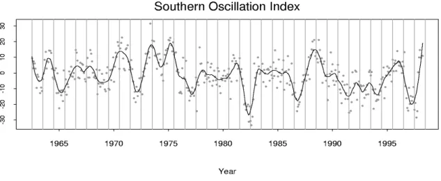
We include the covariatex1,t−1=It whereItdenotes the value of the Southern Oscillation

In-dex (SOI), the standardized anomaly of the Mean Sea Level Pressure (MSLP) between Tahiti and Darwin. IfTk denotes the Tahiti MSLP andDk denotes the Darwin MSLP for monthk,

then the monthly value ofIkis calculated asIk=10(Tk−Dk−µk)/σkwhereµkdenotes the long

term average of(Tk−Dk) for that month andσkdenotes the standard deviation ofTk−Dkfor

that month. (This is known as the Troup SOI.) Figure 1 shows the monthly values between January 1963 and September 1998. There is clearly a lot of random variation in the measure-ment. We have highlighted the underlying trend with a loess curve of degree 2 and span 6%. Negative values ofIk indicate “El Ni ˜no” episodes and are usually accompanied by

sus-tained warming of the central and eastern tropical Pacific Ocean, a decrease in the strength of the Pacific Trade Winds, and a reduction in rainfall over eastern and northern Australia. Positive values of Ik are associated with stronger Pacific trade winds and warmer sea

tem-peratures to the north of Australia (a “La Ni ˜na” episode). Together these are thought to give a high probability that eastern and northern Australia will be wetter than normal. It should be noted that the effect of the Southern Oscillation is greater in Queensland and New South Wales than Victoria (Allan, Lindesay and Parker, 1996). We define It to be the value of the

fitted loess curve at dayt. (Almost identical results are obtained ifItis calculated by linearly

Figure 1:Monthly Southern Oscillation Index with smooth line highlighting the pattern. The smooth line was computed using a loess curve of degree 2 with span of 6%.

We also include the covariate x2,t−1=St =tmod365to model the seasonal variation. The

functiongp+2is constrained to be periodic; that is, we constraingp+2(St)to be smooth at the

boundary betweenSt=365andSt=1.

Thus our occurrence model has

mt(xt−1) =α0+

p

∑

k=1

(αkjt−k+gk(log(yt−k+c)) +gp+1(It) +gp+2(St) +gp+3(t).

Models withp=1,2,3and4were fitted. The results were very similar for allpso we selected

p=1as it simplifies the interpretation.

The smooth term involvingIt was not significantly different from a linear function and so g2(It)was restricted to the linear functiong2(z) =α2z. Becauseg3(St)is a periodic function,

we model it using a Fourier function of the form

g3(St) = m

∑

k=1

[αi,ssin(2πkSt/365) +αi,ccos(2πkSt/365)],

and select the value ofmusing the AIC. (An alternative approach would be to use a periodic smoother.) The smooth termsg1(Yt−1+c)andg4(t)were fitted using smoothing splines. The

final model hadα1=0.26,α2=0.0088,m=3ing3(St)and smoothing parameters df1=4.9

and df4=50where dfidenotes the degrees of freedom for the smooth functiongi. The value

of df1 was chosen by minimizing the AIC, while the smoothing parameter for g4(t) was

selected to allow sufficient flexibility to model changes in the probability of occurrence over a period of two or three years.

The value ofα2was significant (using at-test at the 5% level). However, if the SOI term was

omitted from the model and the other terms re-estimated, the deviance of the model did not change significantly (using aχ2_{test at the 5% level). This anomaly occurs because, if SOI is}

omitted, theg4(t)term can model the variation in SOI. We choose to include SOI because we

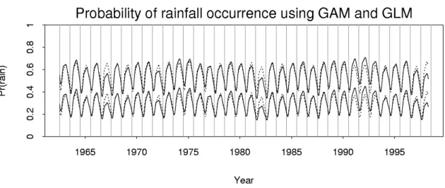
Figure 2: Lower solid line: estimated probability of rain following a dry day. Upper solid line: estimated probability of rain following a day of median intensity (2mm). These estimates are based on the GAM; dashed lines show analogous curves for the GLM.

Figure 2 shows some results for the fitted model. The lower solid line is the estimate of the probability of rain following a dry day (yt−1=0):

Pr(Jt=1|Yt−1=0) =`(α0+g1(logc) +g2(It) +g3(St) +g4(t)).

The upper solid line is the estimate of the probability of rain following a day of median intensity (2mm):

Pr(Jt=1|Yt−1=2) =`(α0+α1+g1(log(2+c)) +g2(It) +g3(St) +g4(t)).

For comparison, analogous curves for a GLM are shown as dashed lines. This model had

mt(xt−1) =α0+α1jt−1+α∗1log(yt−1+c) +α2It+

3

∑

k=1

[αi,ssin(2πkSt/365) +αi,ccos(2πkSt/365)].

Again, the AIC was used to select the number of sinusoidal terms in the seasonal pattern. Higher order AR models were tried but gave very similar results. Note that the GAM allows the modelling of non-seasonal temporal variation whereas the GLM does not.

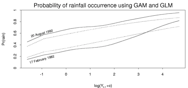
We can also look at the probability of rainfall occurrence as a function of the rainfall intensity of the previous day. Figure 3 shows this relationship for two days in the period of the data. The lower curves are for 17 February 1982 (wheng2(It) +g3(St) +g4(t)was minimized). The

upper curves are for 20 August 1992 (wheng2(It) +g3(St) +g4(t)was maximized). The solid

lines represent the probabilities calculated using the GAM, conditioning on the value oft. The dashed lines show the analogous probabilities as calculated using the GLM.

4.1 Seasonally adjusted occurrence effects

One object of the GAM analysis is to highlight unusual periods of occurrence, relative to “typical” annual occurrence patterns. For instance, comparing the GLM and GAM fits in

Figure 3: Lower solid line: estimated probability of rain on 17 February 1982. Upper solid line: estimated probability of rain on 20 August 1992. Dashed lines show analogous curves for the GLM.

Figure 2 suggests that 1982 had unusually low occurrence and 1990–1993 had unusually high occurrence. To facilitate and quantify such comparisons, we can apply a simple method of seasonal decomposition to decomposemt(xt−1)into a seasonal termst(xt−1)that repeats each

year and represents a “typical” year, and a remainder termrt(xt−1)that represents deviations

from this regular pattern. Let mt(xt−1) =st(xt−1) +rt(xt−1)where st(xt−1) =st+365k(xt−1)for k=1,2, . . .. These effects can be interpreted in terms of odds of rain, so that

Pr[Jt =1|Xt−1=xt−1]

Pr[Jt =0|Xt−1=xt−1]

=exp{mt(xt−1)}=exp{st(xt−1)}exp{rt(xt−1)}.

Thus exp{rt(xt−1)} represents the factor deviation of the odds of rain from the odds in a

typical year, at timet. The seasonally adjusted probability of rain is πa

t(xt−1) =`(s(¯ xt−1) +rt(xt−1))

wheres(¯ xt−1) =₃₆₅1 ∑t365=1st(xt−1), and the seasonal probability of rain is

πs

t(xt−1) =`(st(xt−1)).

Our model provides a convenient estimate ofst(xt−1). We let ˆ

st(xt−1) =αˆ0+αˆ1¯jt−1+g¯1+αˆ2I¯+gˆ3(St) +g¯4

where ¯jdenotes the mean of jt,I¯denotes the mean ofIt,g¯1denotes the mean ofgˆ1(log(yt−1+ c))andg¯4denotes the mean ofgˆ4(t),t=1, . . . ,n.

Figure 4 shows estimates of the seasonal probability of rain,πs

t, and the seasonally adjusted

probability of rain, πat, plotted against time t. The curves for yt−1=0and yt−1=2mm are

shown. The most striking periods of low occurrence are in 1967, 1972, 1982 and 1998. Apart from the most recent drought, these are exactly the droughts in areas encompassing Mel-bourne, as reported by Keating, 1992. The period of highest probability of occurrence is 1992 (which had the greatest number of wet days of any year in the period studied).

Figure 4:Top: Estimated seasonal probability of rain,πts. The horizontal bars show the proportion of

rainy days for each month during the data period. Bottom: seasonally adjusted estimated probability of rain,πa

t. Upper solid lines show curves following a dry day; lower solid lines show curves following

a day of median intensity (2mm). The dashed lines shows the estimated probability of rain further adjusted to show the effect of the SOI.

Our model attempts to separate the non-seasonal temporal variation,g2(It) +g4(t), into two

parts: one due to the SOI and one which is unaffected by the SOI. To help visualize the effect of this separation, the dashed lines in the bottom plot of Figure 4 show the probability of rain predicted by the model after seasonal adjustment and removing the effect ofg4(t). That is,

we plot the estimate of

`(α0+α1jt−1+g1(log(yt−1+c)) +α2I2+g¯3+g¯4).

The resulting curve shows the effect of the SOI on rainfall probability.

The differences between the solid and dashed curves are of interest. For example, in 1967, the solid curve is substantially lower than the dashed curve. This was a period of drought (reflected by the dip in the solid curve) which was not associated with a corresponding low in SOI. The drought of 1982 was associated with the SOI (hence the trough in the dashed curve), but it was more severe than the SOI suggested. Thus, the solid line dips further than the dashed line. The period 1991–1993 is one with unusually high rainfall occurrence that was not associated with a corresponding high in the SOI.

Much of the non-seasonal temporal variation in rainfall probability is being modelled by

g4(t)rather than g2(It). So while the SOI appears to have some effect on the rainfall

Figure 5: Top: Estimated mean intensity of rain following a dry day. Bottom: estimated mean intensity of rain following a day with 30.2mm of rain. Solid lines calculated from the GAM; dashed lines calculated from the GLM.

extreme values of rainfall probability.

5 Modelling intensity

Following the same sorts of modelling procedures as we used for the occurrence process, we can construct GLMs and GAMs for rainfall intensityWt. Recall thatWt≡[Yt|Yt >0], and that

we assume it has distributionG(µ(xt−1),r)whereG(µ,r)denotes a Gamma distribution with

meanµ>0and shape parameterr>0. The fitted model had conditional mean

µt(xt−1) =exp{β0+β1jt−1+h1(yt−1+c) +h2(It) +h3(St) +h4(t)}.

(As with occurrence, we also tried higher order autoregressive terms but they made little difference to the fitted models.) The seasonal term h3 hadm=4 and the bandwidths for h1(yt−1)andh3(t)were 14 and 50 respectively, df1chosen by minimizing the AIC.

The GLM we used had

µt(xt−1) =exp ( β0+β1jt−1+β1∗log(yt−1+c) +β2It+ 4

∑

The sinusoidal terms describe the seasonal pattern in rainfall intensity. The number of sinu-soidal terms was chosen using the AIC.

Figure 6: Mean rainfall intensity (calculated from the GAM) for two days: 24 January 1996 and 10 July 1997. These days were at the maximum and minimum of ˆh2(It) +ˆh3(St) +ˆh4(t)respectively.

Solid lines calculated from the GAM; dashed lines calculated from the GLM.

Figure 5 shows the mean rainfall intensityµt(xt−1)plotted againsttfor two different values

of yt−1. The top plot shows the curve following a dry day (yt−1=0). For comparison, the

analogous curve from the fitted GLM is shown. The bottom plot shows the curve where the previous day has rainfallyt−1=30.2mm. This value ofyt−1provides the maximum value of ˆh1. The GLM curve in the lower plot is clearly biased downwards due to the assumption of

a linear relationship with log(yt−1+c).

Interestingly, the drought of 1982 does not appear to have affected rainfall intensity—it ap-parently was an event mainly involving the frequency of rain, not the amount of rain when it did rain. The summer of 1996–1997 had unusually low rainfall intensity, whereas it was not unusual in the frequency of rain (compare Figure 2). While both years were associated with an El-Ni ˜no event (indicated by low values of the SOI, see Figure 1), the effect appears to have been different.

Figure 6 shows the mean rainfall intensity as a function of log(yt−1+c)for two days. The

value of t was chosen to provide the minimum and maximum values of ˆh2(It) +ˆh3(St) + ˆh4(t). Clearly, the amount of rain on one day,yt−1, has virtually no effect on the amount of

rain on the subsequent day, yt, unlessyt−1 >e3−c≈20mm. In other words, there is little

autocorrelation in the intensity series unless there is a large rainstorm, in which case it will probably extend into the following day. The clearly non-linear relationship demonstrates why there is bias in the GLM estimate of intensity as seen in Figure 5.

The seasonally adjusted mean intensity is calculated in a similar way to that for probability of occurrence described in Section 4.1. The results are shown in Figure 7. Of the major droughts, not all are clearly identified by low intensity. The droughts of 1994 and 1997 appear to have been in periods of low rainfall intensity, but not the drought of 1972. Although the SOI is significant, its effect is small. The major non-seasonal temporal variation in intensity is not associated with the SOI.

Figure 7: Top: Seasonal mean intensity. The horizontal bars show the average rainfall intensity for each month during the data period. Bottom: Seasonally adjusted mean intensity. Lower curves show the mean following a dry day; upper curves show the mean following a day with 30.2mm of rain. The dashed lines shows the probability of rain further adjusted to show the effect of the SOI.

6 Markov Generalized Additive Models for rainfall

We now consider combining the occurrence and intensity models of previous sections to give a model for rainfall amount with a mixed density as given in (2.1). In some applications this combined model will be of most interest since it has units of mm/day while intensity has units of mm/wet day. The fitted amount model yields a mixed density which can be summarized in various ways. For instance, we can calculate the mean ofYt directly from

(2.1) as

E(Yt|Xt−1=xt−1) =πt(xt−1)µt(xt−1).

We are also interested in the marginal mean

Mt =E(Yt|X1,t−1=x1,t−1, . . . ,Xr−p,t−1=xr−p,t−1)

although this is difficult to calculate analytically from the fitted model. Instead we simulate 10,000 sample paths from the model and average across the sample paths to calculateMˆt.

To find the seasonally adjusted mean ofYt, we letsˆ∗t =average(Mˆt+365k)fort=1, . . . ,365and

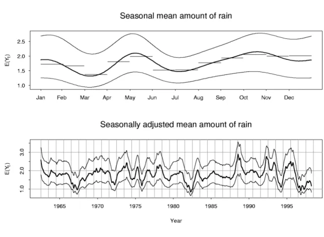
the average is taken overk=0,±1,±2, . . .. Then we smoothsˆ∗_t using a periodic smoother to obtainst, the average rainfall for dayt. Finally, the seasonally adjusted rainfall on daytis rt =Mt−st+s¯t. The results are shown in Figure 8 with the seasonal average (st) shown in the

Figure 8: Top: Seasonal mean amount. Bottom: Seasonally adjusted mean amount. In both graphs the lower curves show means conditional on previous day being dry; the upper curves show means conditional on previous day having median intensity (2mm); the centre (bold) curves show uncondi-tional means. The horizontal lines in the top graph show the average amount for each month in the data period.

Note that there is far less variability in the seasonal mean amount than in the seasonal proba-bility of occurrence or seasonal mean intensity. The probaproba-bility of occurrence is highest in the winter months while the mean intensity is highest in the summer months. These seasonal patterns largely cancel each other out to give a relatively flat daily mean amount across the year. However, the density of amount varies a lot throughout the year, even though the mean is relatively stable. This is seen, for example, in the conditional density functions shown in Grunwald and Jones (1998).

The seasonally adjusted values show that droughts in southern Victoria are more complex than may have previously been understood. Comparing Figures 4, 7 and 8, we note that the drought of 1994, for example, appears to have resulted from lower intensity than usual but that the occurrence was not particularly low for that year. However, the drought of 1982 appears to be more due to low occurrence than low intensity.

Crude estimates of the seasonally adjusted mean curves for amount, intensity and occur-rence could be obtained by relatively simple smoothing techniques. However, the modelling approach we have proposed here has enabled us to go much further in estimating curves conditional on past observations, in estimating the effect of the Southern Oscillation Index on both occurrence and intensity, and in decoupling the effects of occurrence and intensity on rainfall amounts.

6.1 Forecasting

One application of the model presented here is forecasting the series of interest. To produce forecasts, we must estimate the conditional mean functions for the occurrence and intensity models for future times.

This can be done by simulating future sample paths from the model, and then averaging these at each time point. Wherexi−p,t−1is not known in advance (such as with SOI), it must

be replaced by a forecast. The non-seasonal temporal variation must also be forecast as the functions gr+1(t) andhr+1(t) are not defined fort beyond the range of the historical data.

These can be computed by fitting stationary AR models. This approach has the advantages of (1) being able to model the cyclic fluctuations seen in the models for Melbourne’s rainfall, and (2) producing long-term forecasts which converge to the long-term mean (see Makri-dakis, Wheelwright and Hyndman, 1998).

Currently, the Bureau of Meteorology uses forecasts of the SOI to guide their long-term cli-mate prediction. The analysis presented here suggests that that procedure is not going to yield good prediction for southern Victoria because the relationship between SOI and rain-fall is not strong. The method is probably much better for locations in New South Wales and Queensland where the relationship between SOI and rainfall is stronger (Allan, Linde-say and Parker, 1996). However, even there the model presented here will probably lead to better long-term forecasts as it incorporates temporal variation not due to the SOI.

Acknowledgments

Gary Grunwald and Rob Hyndman were supported by Australian Research Council grants. Much of the work by Gary Grunwald was completed when he was in the Department of Statistics, University of Melbourne. The work by Rob Hyndman was done while he was visiting the Department of Statistics, Colorado State University.

References

AITCHISON, J. (1955) On the distribution of a positive random variable having a discrete probability mass at the origin.J. Amer. Statist. Assoc.,50, 901–908.

ALLAN, R., LINDESAY, J. and PARKER, D. (1996) El Ni ˜no: Southern oscillation and climatic variability. CSIRO Publications, Melbourne, Australia.

CLEVELAND, W.S., GROSSE, E. and SHYU, W.M. (1992) Local regression models, in J.M. Chambers and T.J. Hastie (Eds.),Statistical models in S, Wadsworth and Brooks: Pa-cific Grove.

EILERS, P.H.C. and MARX, B.D. (1996) Flexible smoothing with B-splines and penalties

(with discussion).Statist. Sci.,89, 89–121.

GREEN, P.J. and SILVERMAN, B.W. (1994)Nonparametric regression and generalized linear mod-els: a roughness penalty approach. Chapman and Hall: London.

autoregressive structure. Computational Statistics and Data Analysis,28, 171–191.

GRUNWALD, G.K. and JONES, R.J. (1998) Markov models for time series with mixed distri-bution.Environmetrics, to appear.

HASTIE, T.J. and TIBSHIRANI, C. (1990) Generalized additive models. Chapman and Hall: London.

HYNDMAN, R.J., BASHTANNYK, D.M. and GRUNWALD, G.K. (1996) Estimating and visual-izing conditional densities.J. Comp. Graph. Statist.5(4), 315–336.

HYNDMAN, R.J. and YAO, Q. (1998) “Nonparametric estimation and symmetry tests for

con-ditional density functions”. Working paper, Department of Econometrics and Business Statistics, Monash University.

KATZ, R.W. and PARLANGE, M.B. (1995) Generalizations of chain-dependent processes: ap-plications to hourly precipitation.Water Resources Research,31, 1331–1341.

KEATING, J. (1992)The drought walked through: a history of water shortage in Victoria. Depart-ment of Water Resources Victoria: Melbourne.

MAKRIDAKIS, S., WHEELWRIGHT, S. and HYNDMAN, R. (1998)Forecasting: methods and ap-plications. John Wiley & Sons: New York.

MCCULLAGH, P. and NELDER, J. (1989)Generalized linear models. 2nd ed., Chapman and Hall: London.

STERN, R.D. and COE, R. (1994) A model fitting analysis of daily rainfall data (with