SIMULTANEOUS INFERENCE IN GENERALIZED LINEAR MODEL SETTINGS
By
AMY WAGLER
Bachelor of Science in Mathematics University of Texas of the Permian Basin
Odessa, Texas, USA 1995
Master of Science in Statistics Oklahoma State University Stillwater, Oklahoma, USA
2003
Submitted to the Faculty of the Graduate College of Oklahoma State University
in partial fulfillment of the requirements for
the Degree of
DOCTOR OF PHILOSOPHY July, 2007
COPYRIGHT c By
AMY WAGLER July, 2007
SIMULTANEOUS INFERENCE IN GENERALIZED LINEAR MODEL SETTINGS
Dissertation Approved: Dr. Melinda McCann Dissertation Advisor Dr. Stephanie Monks Dr. Mark Payton Dr. Wade Brorsen Dr. A. Gordon Emslie Dean of the Graduate College
ACKNOWLEDGMENTS
There are many I would like to thank for assistance, reassurance and inspiration during the time I worked on this dissertation. First, I would like to thank the entire Department of Statistics at Oklahoma State University including all of the faculty members, staff, and students. I appreciate your kindness and concern for me. Of the faculty members, I would specifically like to thank my committee members, Dr. Stephanie Monks, Dr. Mark Payton, and Dr. Wade Brorsen, for the time and effort they put into this research project. Most importantly, I would like to thank my advisor, Dr. Melinda McCann, for her support and encouragment, perseverance in research, and friendship. I was fortunate to have an advisor such as you. I would also like to thank Trecia Kippola, Tracy Morris, and Janae Nicholson who listened to my many complaints and were just good friends.
The most emphatic thanks I reserve for my family, who are always loving and supportive. My Mom, Dad, and sisters for believing I could do this even when I didn’t believe. Most of all, I would like to thank Ron, my husband, and Olive, my daughter. When I needed help, encouragement, or a baby-sitter, my husband was always there. When I was frustrated and feeling down, a smile from Olive was all I needed to put things in perspective. Thank you and I love you both.
TABLE OF CONTENTS
Chapter Page
1 INTRODUCTION 1
2 The GLM and Estimated Quantities 6
2.1 The Expected Mean Response . . . 8
2.2 The Odds Ratio . . . 10
2.3 Other Quantities . . . 12
2.4 Interval Estimation from GLMs . . . 14
2.4.1 Logistic Regression Model . . . 14
2.4.2 Reference Coding for Logistic Regression . . . 17
2.4.3 Loglinear or Poisson Model . . . 18
3 Inferences on Quantities Estimated from a GLM 22 3.1 Inference on the Mean Response . . . 22
3.1.1 Previous Methods . . . 23
3.1.2 Proposed Methods . . . 31
3.2 Bounds for Simultaneously Estimating Functions of Model Parameters 39 3.2.1 Previous Methods . . . 40
3.2.2 Proposed Methods . . . 42
4 Simulations 49 4.1 Expected Response Function Simulations . . . 49
4.1.1 Expected Response Function Simulation Results . . . 51
4.2.1 Functions of the Parameters Simulation Results . . . 63
5 CONCLUSIONS 65 5.1 Application of Proposed Methods . . . 65
5.1.1 Diabetes among Pima Women . . . 65
5.1.2 Depression in Adolescents . . . 66
5.2 Overall Conclusions . . . 68
5.2.1 Recommendations for Estimating the Mean Response . . . 68
5.2.2 Recommendations for Estimating the Parameters . . . 69
5.3 Future Research . . . 70
BIBLIOGRAPHY 72 A FIGURES 75 B Moments of Binomial and Poisson Random Variables 92 B.1 The Binomial Random Variable . . . 92
B.2 The Poisson Random Variable . . . 93
C Restricted-Scheff´e Methodology 94
D SCR Methodology 97
E Fortran Code: Piegorsch-Casella PMLE for the Mean Response 100
F Fortran Code: SCR PMLE for the Mean Response 123
G Fortran Code: Piegorsch-Casella PMLE for the Parameters 150
LIST OF TABLES
Table Page
1.1 Maternal Stress Relative Risks and 95% Confidence Intervals . . . 3
2.1 Sample Contingency Table . . . 11
2.2 Examples of Estimated Odds Ratios . . . 18
5.1 Intervals for Proportion of Pima Women with Diabetes . . . 66
LIST OF FIGURES
Figure Page
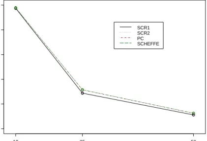
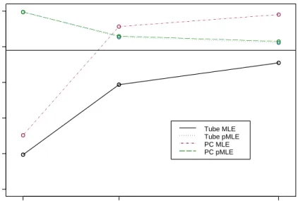
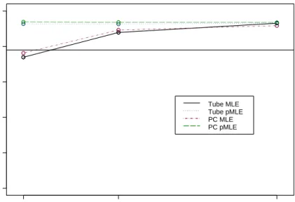
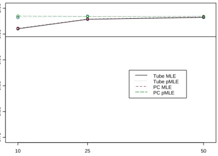
4.1 MLE and PMLE SCR Intervals with wide range . . . 51
4.2 pMLE Intervals Logit-Wide Range B=1 . . . 52
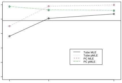
4.3 MLE and PMLE SCR Intervals with wide range . . . 54
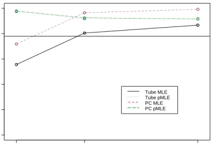
4.4 MLE and PMLE SCR Intervals with wide range . . . 54
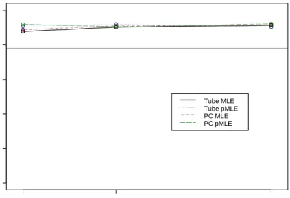
4.5 MLE and PMLE SCR Intervals with wide range . . . 55
4.6 MLE and PMLE SCR Intervals with narrow range . . . 55
4.7 MLE and PMLE SCR Intervals with narrow range . . . 56
4.8 MLE and PMLE SCR Intervals with narrow range . . . 56
4.9 MLE and PMLE SCR Intervals with narrow range . . . 57
4.10 MLE and PMLE SCR Intervals with narrow range . . . 57
4.11 MLE and PMLE SCR Intervals with narrow range . . . 58
4.12 MLE and PMLE SCR Intervals with narrow range . . . 58
4.13 MLE and PMLE SCR Intervals with narrow range . . . 59
4.14 MLE and PMLE SCR Intervals with narrow range . . . 59
4.15 MLE and PMLE SCR Intervals with narrow range . . . 60
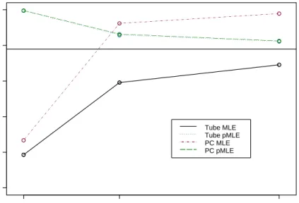
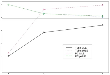
4.16 MLE and PMLE SCR Intervals for the Parameters . . . 63
4.17 MLE and PMLE SCR Intervals for the Parameters . . . 64
A.1 MLE Intervals Logit-Wide Range B=1 . . . 75
A.2 MLE Intervals Logit-Wide Range B=2 . . . 76
A.3 MLE Intervals Logit-Wide Range B=3 . . . 76
A.5 MLE Intervals Logit-Narrow Range B=1 . . . 77
A.6 MLE Intervals Logit-Narrow Range B=2 . . . 78
A.7 MLE Intervals Logit-Narrow Range B=3 . . . 78
A.8 MLE Intervals Logit-Narrow Range B=4 . . . 79
A.9 MLE Intervals Poisson-Wide Range B=1 . . . 79
A.10 MLE Intervals Poisson-Wide Range B=2 . . . 80
A.11 MLE Intervals Poisson-Wide Range B=3 . . . 80
A.12 MLE Intervals Poisson-Narrow Range B=1 . . . 81
A.13 MLE Intervals Poisson-Narrow Range B=2 . . . 81
A.14 MLE Intervals Poisson-Narrow Range B=3 . . . 82
A.15 pMLE Intervals Logit-Wide Range B=2 . . . 82
A.16 pMLE Intervals Logit-Wide Range B=3 . . . 83
A.17 pMLE Intervals Logit-Wide Range B=4 . . . 83
A.18 pMLE Intervals Logit-Narrow Range B=1 . . . 84
A.19 pMLE Intervals Logit-Narrow Range B=2 . . . 85
A.20 pMLE Intervals Logit-Narrow Range B=3 . . . 85
A.21 pMLE Intervals Logit-Narrow Range B=4 . . . 86
A.22 pMLE Intervals Poisson-Wide Range B=1 . . . 86
A.23 pMLE Intervals Poisson-Wide Range B=2 . . . 87
A.24 pMLE Intervals Poisson-Wide Range B=3 . . . 87
A.25 pMLE Intervals Poisson-Narrow Range B=1 . . . 88
A.26 pMLE Intervals Poisson-Narrow Range B=2 . . . 88
A.27 pMLE Intervals Poisson-Narrow Range B=3 . . . 89
A.28 MLE Intervals for the Parameters - Logit . . . 89
A.29 MLE Intervals for the Parameters - Poisson . . . 90
A.30 pMLE Intervals for the Parameters - Logit . . . 90
CHAPTER 1
INTRODUCTION
Modern epidemiological and medical research routinely employs generalized linear modeling. These models can be helpful in understanding what behaviors or traits can influence the incidence of a particular disease or characteristic. For example, logistic regression models provide a means of relating the incidence of some trait or disease to a set of possible predictor variables, while loglinear models help us understand associations between a trait and predictor variables.
After building a generalized linear model(GLM), one typically wishes to estimate particular quantities of interest such as response probabilities, odds ratios, or relative risks. Customarily, these are reported via confidence intervals or confidence bounds using some pre-specified level of significance for each inference. For example, using a loglinear model, one could report 100(1−α)% confidence intervals for each rela-tive risk resulting from the model. Using one-at-a-time intervals is appropriate when the investigators are not making overall conclusions about the quantities of interest. For example, if the aforementioned loglinear model was estimated and 100(1−α)% confidence intervals for the relative risks were reported, conclusions about each in-dividual relative risk could be made, but any statements comparing these relative risks would inflate the assumed α error rate. Research on simultaneous estimation procedures for quantities from generalized linear models has received little attention beyond very routine treatments, such as making Bonferroni adjustments to the usual confidence interval or constructing Scheff´e intervals. However, recent advances made in simultaneous inference for linear models may be applied in the generalized linear
model setting. Additionally, further improvements may be made by utilizing some unique properties of the estimated parameters from generalized linear models. I plan to present the justification for employing these simultaneous inference methods in the generalized linear model setting and, via simulation, compare their performance. Thus, the objective of this study is to develop simultaneous interval based procedures that will estimate functions of linear combinations of the parameters of a general-ized linear model. Specifically, this includes simultaneously estimating the expected response function, odds ratios, and relative risks from generalized linear models.
Overall, attention is focused on quantities that are estimated from a GLM, not the estimation of the GLM itself. Obviously, the performance of any of these procedures will be influenced by how well the model is estimated, but this dissertation will assume the model is well estimated. Additionally, all of the procedures developed in this paper involve constructing interval estimates. Often, procedures that account for multiplicity employ hypothesis tests to make overall conclusions about a set of data. It is more appropriate in the applications I will discuss to use simultaneous intervals instead of stepwise procedures, since I wish to not only detect statistical differences between quantities, but also to assess the practical significance of these differences. Thus, all methods discussed are interval-based procedures.
Before presenting the details of generalized linear models, a practical example of the implementation of a GLM may provide a frame of reference. A 2003 study from the American Journal of Epidemiology explored the relationship between ma-ternal stress and preterm birth [1]. Several previously identified sources of mama-ternal stress, such as high incidence of life events, increased anxiety, living in a dangerous neighborhood, and increased perception of stress, were explored for any association with preterm births. Specifically, the study focused on predicting the prevalence of preterm birth among pregnant women aged 16 or older from two prenatal clinics in central North Carolina. Upon admission to the study, women were asked to complete
Table 1.1: Maternal Stress Relative Risks and 95% Confidence Intervals
Life Events Stress RR 95% CI No Stress 1.00
Med-Low Stress 1.5 (1.0, 2.2) Med-High Stress 1.4 (0.9, 2.1) High Stress 1.8 (1.2, 2.7)
questionnaires in addition to completing a psychological instrument. Also, several blood, urine, and genital tract tests were conducted in order to assess the physical health of the candidates. In all, 2,029 women were eligible, recruited, and completed the preliminary tests in order to participate in the study. Of these participants, 231 delivered preterm, less than 37 weeks gestation. A loglinear model was employed to assess the relationship between the sources and levels of maternal stress and preterm birth. As a result, the authors considered the resulting model relative risks for each individual stress factor or level of a stress factor and its association with preterm birth. Additionally, 95% confidence intervals were computed for each relative risk. The relative risk will be discussed in detail later, but note that for this study each relative risk is the risk of preterm birth for an individual with one particular maternal stress factor relative to the risk of preterm birth for an individual with none of the other identified sources of maternal stress present. Thus a large relative risk for a particular source of maternal stress indicates a strong association between that stress factor and preterm birth. In general, other quantities derived from the generalized linear model may also be of interest. Table 1.1 contains results from the preterm birth study discussed, though these results have been simplified from the actual im-plemented model for ease of presentation. In particular, the relative risks for different levels of stress due to general life events is presented. As previously discussed, note
that the 95% confidence intervals for each relative risk presented in Table 1.1 estimate the risk of preterm birth for each individual subject to a particular level of a maternal stress factor (life event stress) with reference to the control (the case with no identified source of maternal stress). For this scenario, one-at-a-time inferences are reasonable if the researcher wishes to answer questions such as, “how does the presence of one source of maternal stress affect the risk of preterm birth?” Note that this question is only concerned with the presence of a particular stress factor and how it affects the incidence of preterm births. If one wishes to make any overall conclusions comparing how the multiple sources of maternal stress affect the risk of preterm birth, then an-other estimation procedure that accounts for multiplicity needs to be implemented. For instance, in the preterm birth study, the researchers reported the above relative risks and confidence intervals, and then remarked that “(w)omen in the highest neg-ative life events impact quartile had the highest risk (RR=1.8, 95% CI: 1.2, 2.7); however, the middle categories did not show increasing risk with increasing measures of stress.” This kind of conclusion is inappropriate given that the researchers only computed one-at-a-time 95% confidence intervals for the relative risks. Therefore, this is a case that would benefit from simultaneous inference on the relative risks.
As another example where simultaneous inference would be appropriate, consider the case where the researcher wishes to identify the set of the sources and levels of maternal stress that are significantly associated with preterm birth. In this case the one-at-a-time intervals are again inappropriate. In order to make this kind of conclu-sion, the researcher needs to determine which groups of relative risks are significantly different from 1. If the researcher additionally wants to determine the practical sig-nificance of the differences between the varying sources and levels of maternal stress and the control, then confidence intervals with a multiplicity adjustment are required. Stepwise procedures are not adequate as they only determine where statistically sig-nificant differences exist, but do not provide a way to estimate the scale of these
differences. Additionally, it is often desirable to make conclusions such as “if the sub-ject has one level of a predictor variable, then he is twice as likely to have the disease than if he has any other level of that predictor variable”. Many other examples of similar conclusions could be given, but generally, these conclusions are comparing one parameter to another and the desired outcome is to somehow relate these parameters. Thus, if one wishes to make any comparisons of these parameters, it is desirable to control the overall type I error rate by accounting for the multiplicity of inferences.
In the following chapters, I will present the motivation for simultaneous inference of certain parameters and outline both the current methodologies and my proposed methodologies. Additionally, the simulation results of the proposed methods are presented and analyzed. Specifically, in chapter two, I present the generalized linear model and the typical quantities that are estimated from the model, and discuss why simultaneous inference of these quantities is essential in some situations. Additionally, I review some methods for computing one-at-a-time confidence intervals on various quantities resulting from generalized linear models. In chapter three, I outline the current methodologies used for simultaneously estimating various functions resulting from generalized linear models, and I propose four new methods to estimate these parameters from GLMs. In chapter four, I summarize how I evaluated these new methods using simulation and present the simulation results. Finally, I propose some future research questions regarding simultaneous estimation of a GLM and present some applications of the new methods in the concluding chapter.
CHAPTER 2
The GLM and Estimated Quantities
There are several generalized linear models (GLM) that permit estimates, such as the odds ratio or relative risk, where multiplicity adjustments often seem warranted. Some of these models include the logistic regression model, loglinear model, Poisson regression model, and the probit or complementary log-log model. In general, a GLM can be expressed as
Yi=g−1(xi′β+ǫi), i= 1, . . . , n (2.1)
or alternatively,
φi =g(E(Yi|xi)) =x′iβ, i= 1, . . . , n (2.2) whereg links the expected response, E(Yi|xi), to φi, with xi the vector of covariates corresponding toYi,βthek×1 vector of regression parameters, andǫi independently and identically distributed random variables. In the later sections,Y = (Y1, . . . , Yn)′ is the vector of responses andX = (x1, . . . ,xn)′ is the full rank matrix of predictor variables. Each GLM corresponds to a particular link functiong, typically called the canonical link when it transforms the mean to the natural parameter. In general, the maximum likelihood estimate (MLE) of the regression parameters is denoted
ˆ
β= ( ˆβ1, . . . ,βˆk). The MLE is asymptotically multivariate normal with mean β and covariance matrix
where W is a diagonal matrix with diagonal elements wi = (∂µi/∂φi)2/var(Yi) for
µi =E(Yi|xi) and φi in (2.2). Thus, ˆ
β∼· Nk(β,V). (2.4)
We can estimate the covariance matrix, V, by ˆ
V = ˆcov( ˆβ) = (X′W Xˆ )−1 (2.5) with ˆW =W|β= ˆβ. Further results will require the estimated covariance of x′iβ for a given xi vector with k known elements. This is given by
ˆ
σ2GLM(xi) =
q x′
iV xˆ i, i= 1, . . . , n. (2.6)
At times I will need to refer to a linear model in this proposal. A linear model is generally given by
Yi =x′iθ+ǫi, i= 1, . . . , n (2.7)
or alternatively,
E(Y) =Xθ (2.8)
where θ is the vector of regression parameters, Y and X are as previously defined,
and ǫi ∼ iid N(0, σLM2 ). The MLEs forθ = (θ1, . . . , θk) are denoted θˆand
ˆ
θ ∼Nk(θ, σLM2 F) (2.9)
whereσ2
LM is the variance of the model residuals for a linear model andF = (X′X)−1. Whenever a linear model is referenced in this paper, the notation presented above will be utilized.
As discussed previously, the objective of this research is not to merely estimate a GLM, but to simultaneously estimate quantities derived from a GLM. There are many natural quantities that can be of interest when modeling data with a GLM. These include measures such as the expected mean response, the odds ratio, the relative
risk, and possibly others. While the focus of this paper is on the estimation of these quantities from GLMs, it should be mentioned that they may be estimated directly from the data. I will first present these measures in general, and then discuss them specifically in the context of generalized linear models.
2.1 The Expected Mean Response
The expected mean response is a generic term for either the response probability or the mean response. Depending on the sampling distribution of the data, either one or the other is of interest. For example, if we assume binomial sampling, the expected mean response function is the probability of a success for a given level of the predictor variables, or the response probability. When a Poisson sampling scheme is assumed, the expected mean response is the average for a particular cell in the contingency table, or the mean response.
A response probability is the proper quantity of interest if one wishes to under-stand the probability of developing a disease or another characteristic for a given set of predictor variables that are believed to be associated with the disease. For example, a response probability could be used to inform a particular patient of their probability of developing a particular disease given their history and profile. With respect to the preterm birth example, if a doctor has a patient known to be experiencing a major life event, such as a death in the family, then she could ascertain that patient’s risk of preterm birth and take appropriate measures.
Conversely, the mean response might be used in a situation where a clinician has recorded a host of risk factors for a particular disease and wishes to predict how many of the subjects will develop the disease. This communicates how many patients on average will or will not develop a certain characteristic. In the context of the preterm birth example, the Poisson mean response could be used to estimate how many subjects out of the total sample size will experience a preterm birth. The
Poisson mean response is simply estimated directly from the frequencies given in a contingency table when it is not estimated from a model.
In general, a one-at-a-time 100(1−α)% confidence interval for the response prob-ability is given by ˆ πi±zα/2( ˆvar( ˆπi))1/2 (2.10) where var( ˆπi) = πi(1−πi) mi and ˆvar(ˆπi) = ˆ πi(1−ˆπi)
mi . (Note that confidence intervals on
the mean response for Poisson sampling distribution models are not typically com-puted.) This one-at-a-time confidence interval forπi is often employed to estimate an expected mean response for binomial or multinomial sampling scenarios. If the re-searcher simply wants to know how a particular level of the predictor variables affects the incidence of disease, this is all that needs to be calculated. First, consider the case where the predictor variable is categorical, as in the preterm birth example. Suppose a clinician wishes to estimate the risk of preterm birth for a particular patient in her clinic. Then the one-at-a-time interval would be adequate. Alternatively, consider a scenario where a researcher wants to make some kind of overall conclusion about the relationship between all the sources and levels of maternal stress and preterm birth. For example, suppose the researcher wishes to compare the risk of preterm birth for all the maternal stress factors and their levels. In order to simultaneously estimate these differences, the researcher would need to employ some kind of proce-dure that accounts for the multiple inferences being made. Additionally, it would be of practical interest to identify a group of maternal stress factors and levels that are “most associated” with preterm birth and another group of maternal stress factors and levels that are “least associated” with preterm births. This too would necessitate a procedure that adjusts for multiplicity while also providing interval estimates of the response probabilities for each stress factor. Finally, consider the case where the researcher would want to compare the probability of preterm birth for each maternal stress factor or level with the probability of preterm birth for a control or reference
level. In this example, the reasonable reference level would be subjects that have no identified sources of maternal stress. Again the appropriate procedure would adjust for multiplicity.
Now consider the case where the predictor variable is continuous. Often, with a continuous predictor variable, a specific range of the domain is of particular interest. For example, if we added a continuous measure of each patient’s prepregnancy body mass index (BMI) in the preterm birth study, we might have particular interest in BMI’s less than 19.8 (underweight), 19.8 to 26.0 (normal weight), 26.0 to 29.0 (over-weight), and over 29.0 (obese). It may be of interest to compare the expected number of preterm birth cases for subjects within these BMI groups within a particular ma-ternal stress factor group. In order to make conclusions such as the obese patients have the largest number of preterm birth cases, interval estimates need to be used that account for the multiple inferences being made. The methods I propose will adjust for this kind of multiplicity.
2.2 The Odds Ratio
The odds ratio is a widely used measure in epidemiological and medical applica-tions. The odds ratio is generally defined as the ratio of the odds of a characteristic (or disease) occurring in one group to the odds of it occurring in another group. With reference to the preterm birth study, odds ratios could have been computed that would estimate the relative odds of preterm birth for a particular level of a ma-ternal stress factor to the odds for those mothers with no identifiable stress factors. Thus, an odds ratio of 2.11 for mothers who live in a neighborhood perceived to be dangerous, would be interpreted as: the odds of delivering a preterm infant when living in a neighborhood that is perceived to be dangerous is 2.11 times greater than the odds of having a preterm infant when a subject is not exposed to any identifiable sources of maternal stress.
Table 2.1: Sample Contingency Table
X =x1 X =x2
Y = 1 a b m1
Y = 0 c d m2
n1 n2 n
The sample odds ratio can easily be computed from the raw data and is given by ˆη = ad
bc for counts as given in Table 2.1 irrespective of which sampling model (binomial, multinomial, or Poisson) is assumed for the cell counts. For large samples, again under all sampling models, the log odds ratio,log(ˆη) is asymptotically normal with mean log(η) and estimated standard error ˆσlogηˆ = (1a +1b + 1c + 1d)1/2. Thus, a
100(1−α)% one-at-a-time large sample confidence interval for the log odds ratio is given by
log(ˆη)±zα/2σˆlog(ˆη). (2.11)
Exponentiating the lower and upper bounds of this interval yields confidence bounds for the odds ratio.
It is common to see one-at-a-time confidence intervals for odds ratios reported along with their point estimates. Suppose a researcher wants to report the estimated odds ratio for a particular patient profile with confidence limits. For example, in the preterm birth example, she may want to report the odds ratio of preterm birth for those exposed to a particular maternal stress factor compared to those with no identifiable maternal stress factors. In this case, the one-at-a-time intervals are ap-propriate. Alternatively, consider the case where the researcher wants to identify which, if any, of the maternal stress factors or levels of a stress factor are statistically associated with a preterm birth or to identify a set of stress factors or level of a stress
factor whose association with preterm birth is larger than that for no stress factors present. The one-at-a-time intervals will not suffice for these kinds of questions as there are multiple inferences being made. In order to control the type I error rate, a simultaneous estimation procedure should be utilized. Additionally, the researcher may wish to compare the odds of preterm birth for any maternal stress factor to the odds of preterm birth for all other sources of maternal stress. In order to do this, a multiple comparison procedure must also be utilized as the researcher actually wants to compare the probabilities of preterm birth across all the possible sources of ma-ternal stress. It is tempting to make overall conclusions about the odds ratios when reporting estimated odds ratios via one-at-a-time confidence intervals. However, the error rate associated with these overall conclusions based on multiple one-at-a-time intervals is not controlled, or even known. In this case, a method that simultaneously estimates the parameters is warranted.
2.3 Other Quantities
Another quantity frequently reported is the relative risk. The relative risk com-municates the risk of developing a disease at one level of the predictor variable relative to another level of the predictor variable. An example of a study employing relative risks is the preterm birth study. In Table 2, the estimated relative risk would be given by ˆγ = a/n1
b/n2 where the counts are as in Table 2.1. Suppose a researcher reports that
the estimated relative risk of preterm birth is 1.75, given the subject lives in a neigh-borhood perceived to be dangerous. Thus the proportion of those that experience a preterm birth among those that live in the dangerous neighborhood is estimated to be 1.75 times the proportion of those who experience a preterm birth among those with no identified sources of stress. Again, the log scale is often utilized and large sample derivations show that the log of the sample relative risk,log(ˆγ) is asymptoti-cally normal with meanlog(γ) and estimated standard error ˆσlog(γ) = (1ˆπ−1nˆπ11+1ˆπ−2nˆπ22)1/2
where ˆπi for i = 1,2 is the estimated probability of disease among those in group i andni is the sample size for groupi= 1,2. Thus, the 100(1−α)% confidence interval for the log relative risk is
log(ˆγ)±zα/2σˆlog(ˆγ). (2.12)
These resulting bounds may be exponentiated in order to obtain confidence limits on the relative risk.
It is sufficient to report an estimated relative risk via a one-at-a-time confidence interval when a researcher only needs to understand how one level of the predictor variable affects the incidence of disease. The preterm birth study reported relative risks and the associated confidence intervals, thus only individual inferences about each source of maternal stress or level of a maternal stress factor relative to the case with no source of stress can be made. However, suppose a researcher wishes to pick out which risk factor or level of a risk factor contributes most to a disease or condition, or obtain ranking information for the sources and levels of maternal stress with respect to risk of disease or condition. As estimation is still also of interest, multiplicity adjustments need to be made to the confidence intervals.
In addition to the relative risk, other quantities should be considered as well. For example, many epidemiological researchers find the attributable proportion a useful measure. Suppose we have a disease and several risk factors for that disease. Then the attributable proportion would be the probability that a diseased individual in the given risk factor has the disease because of that risk factor [2]. This is of interest when there are multiple risk factors for a disease. Thus, this measure is of particular interest in case-control studies where the incidence of disease is related to several risk factors as it allows the researcher to understand how much the disease could be reduced by eliminating a particular risk factor.
One-at-a-time confidence intervals can also be utilized to estimate the attributable proportions. Model-based confidence interval formulas can be computed on the usual
attributable proportion. Often transformations of the relative risk are utilized to com-pute bounds on the attributable proportion since they can be more efficient asymptot-ically. However, the MLE-based interval performs adequately [3] and is more easily adjusted for simultaneous inference in the sequel. Thus, a one-at-a-time confidence interval for the attributable proportion, denotedκ, is given by,
ˆ
κ±zα/2×varˆ (ˆκ)1/2 (2.13)
where zα/2 is the z critical value that gives 100(1 − α)% confidence. (Details for
computing ˆvar(ˆκ) are given in [4].)
Again, this interval is all that is required in many applications. However, if the researcher wishes to compare the attributable proportions for a group of risk factors, an adjustment for multiplicity would be necessary. This might be necessary if, for example, one wished to understand which risk factor should be focused on most for prevention of the disease. Here we would want to identify the largest attributable proportion and focus on disease prevention via reducing the effect of that risk factor.
2.4 Interval Estimation from GLMs
Though we have introduced notation for both linear models and GLMs, the rest of this section focuses on the particular GLMs utilized to illustrate the results in this paper. While the methods derived apply to any GLM, particular attention will be devoted to the logistic and Poisson models due to their applicability and popularity.
2.4.1 Logistic Regression Model
The logistic regression model is widely used in epidemiological and health science applications. The predictor variable in a logistic regression model can be either a single variable or a vector of variables. Thus, letxi = (xi1, xi2, . . . , xik) be a vector of
is the number of predictor variables. Thus,xi is theith vector of predictor variables. Recall that for qualitative covariates, the xi’s would be defined as appropriate indi-cator variables. For example, in the preterm birth study xi could be the maternal stress vector of predictor variables with binary elements indicating the presence of a particular source or level of a source of maternal stress. Thus, if the ith case is a patient exposed only to dangerous neighborhoods as a source of maternal stress, we would code xi = (1,1,0,0,0, . . . ,0) where the first element has a 1 for the intercept term, the second place has a 1 to indicate the presence of stress in the form of a dangerous neighborhood, and the other elements of the vector are 0 indicating the patient was not exposed to the other sources of maternal stress. A logistic regression model assumes that the probability of a success for theith observation isπ(xi) where
π(xi) =P[Yi = 1] = ex′ iβ 1 +ex′ iβ = eβ1xi1+...+βkxik 1 +eβ1xi1+...+βkxik, i= 1, . . . , n. (2.14)
The matrixX, as previously defined, contains information relating to the predicted value, Y, for the model. Alternatively, we can express this model as
φ(xi) =logit[π(xi)] = ln[ π(xi)
1−π(xi)] =x
′
iβ, i= 1, . . . , n. (2.15)
Now let the MLE of π(xi) be denoted ˆπ(xi). We will make the usual assump-tion that the Yi random variables are independent and binomially distributed with parameters mi (assumed known) and π(xi) given by (2.14), i = 1, . . . , n. Thus,
W = diag[miπ(xi)(1−π(xi))], i = 1. . . , n and the asymptotic distribution of the MLE of β is given by (2.4). For ˆW = diag[miπˆ(xi)(1 −πˆ(xi))], i = 1, . . . , n, the estimated covariance matrix of ˆβ is given by (2.5).
When it is assumed that a logistic regression model is appropriate, the typical quantities of interest are the coefficients of the regression model, or the log odds ratios, βi, i= 1, . . . , k, and the response probabilities, π(xi). These quantities relate to what was generally referred to as the expected response function. In particular, the
expected response function for a logistic regression model is the response probability since this model assumes binomial sampling.
When considering response probabilities for single experimental units, one-at-a-time confidence intervals seem appropriate. (Confidence intervals provide addi-tional information about the precision of the estimated response probability, so are often preferable to point estimates.) An appropriate confidence interval on the
logit(π(xi)) = x′iβ is computed by
x′iβˆ±z1−α/2σˆGLM(xi) (2.16)
where z1−α/2 is a z-percentile and ˆσGLM(xi) is given by (2.6) with ˆW as previously defined. Let the upper and lower limits of (2.16) be denoted byULOGIT and LLOGIT, respectively. Then we can apply the anti-logit and obtain bounds on the response probability. Thus, a 100(1−α)% confidence interval for the response probability is given by exp(LLOGIT) 1 +exp(LLOGIT) , exp(ULOGIT) 1 +exp(ULOGIT) . (2.17)
Another quantity of interest from a logistic regression model is the odds ratio. One-at-a-time large sample confidence intervals can easily be constructed on the log odds ratios, as they are linear functions of the k logistic regression coefficients, β. Thus we may utilize the asymptotic multivariate normal distribution of the maximum likelihood estimates of thesek logistic regression coefficients, given by (2.4), to obtain large sample confidence intervals for the appropriate odds ratios. For illustration, suppose a particular odds ratio is given byexp(ciβ) for ci = (ci1, . . . , cik), a vector of
appropriate constants. Then a one-at-a-time large sample confidence interval for this particular odds ratio is given by
exp{ciβˆ−zα/2σˆGLM(ci)}, exp{ciβˆ+zα/2σˆGLM(ci)}
(2.18) where ˆσGLM(ci) is given by (2.6). Typically, in epidemiological applications, the logistic regression model employed for computing the model-based odds ratios utilizes
reference coding. When reference coding, as explained below, is utilized, special care must be taken in interpreting the model-based odds ratios.
2.4.2 Reference Coding for Logistic Regression
If a logistic regression model is employed for a categorical predictor variable, the design coding typically used necessitates that one of the levels ofxbe a reference level. Then odds ratios that result from the model coefficients are observed and compared to that reference level. Most often the reference level is a true control, but at times the reference level is arbitrary. When the reference level is informative, we may wish to: (1) estimate all the odds ratios relative to the reference level simultaneously, thereby allowing the researcher to assess the practical significance of any observed difference from the reference level while also providing the ability to evaluate which non-reference levels are significantly greater than or less than the reference level and (2) make comparisons for a pre-specified set of contrasts of the odds ratios. If the reference level is arbitrary, it seems reasonable to simultaneously compute all odds ratios or all odds ratio differences and then emulate one of the two scenarios described above. Again, if we wish to assess the practical significance of any estimates we need to estimate these quantities simultaneously rather than utilize a stepwise procedure. Note that for both above cases, when there is only one categorical predictor variablex, then all inference procedures performed on the odds ratios resulting from the logistic regression model are equivalent to any similar analysis performed on the crude data in contingency table format. Differences will occur in models with multiple covariates.
The standard method for computing the odds ratios resulting from a logistic regression model using reference coding for the design matrix is to exponentiate the appropriate linear combinations of the estimated regression coefficients. For example, if we have a logit model such as (2.15), where there arek levels for our single predictor variable, then we can utilize the explanatory variablesx1, . . . , xk−1 with the covariate
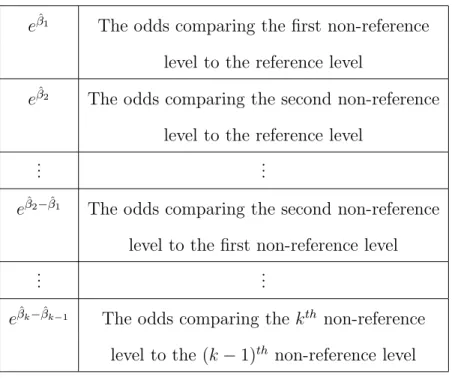
Table 2.2: Examples of Estimated Odds Ratios
eβˆ1 The odds comparing the first non-reference
level to the reference level
eβˆ2 The odds comparing the second non-reference
level to the reference level
... ...
eβˆ2−βˆ1 The odds comparing the second non-reference
level to the first non-reference level
... ...
eβˆk−βˆk−1 The odds comparing the kth non-reference
level to the (k−1)th non-reference level
vector at the reference level of our predictor variable equal to 0, that is, x1 = . . .=
xk−1 = 0. Thus, x1, . . . , xk−1 would be defined as indicator variables for the k−1
non-reference levels of our predictor variable. When this model is assumed, then we can interpret eβˆ1 as follows: the odds that Y = 1 for the first non-reference
level is eβˆ1 times greater than that for the reference level. Table 2.2 illustrates other
estimated odds ratios and their corresponding interpretations. The estimated odds ratios defined in Table 2.2 could then be utilized to construct confidence intervals that would aid in interpreting the model.
2.4.3 Loglinear or Poisson Model
Another model often employed in epidemiological studies is the loglinear model. The loglinear model relates the counts of a Poisson or multinomial distribution to a set of covariates. It may assume the total sample size is random or fixed, depending on whether the model assumes Poisson or multinomial sampling, respectively. For an
I×J contingency table letN =I×J. Note that the number of cells in a contingency table, N, is distinct from the sample size or number of observations, denoted n, although they can be equal. Whenever the number of observations, n, is fixed, we have multinomial sampling for Yi, i= 1, . . . , N −1. However, when the sample size
n is not fixed, we usually assume Poisson sampling for Yi, i = 1, . . . , N. For ease in notation let n∗ = N −1 for multinomial sampling and N for Poisson. Then the
loglinear model is
log(µ(xi)) = x′iβ, i= 1, . . . , n∗ (2.19) where E(Y) = µ = (µ(x1), . . . , µ(xn∗))′ is the vector of expected counts of the
respective cells of the contingency table,xi is a 1×k vector of covariates as described in (2.2), andβ is ak-dimensional vector of model parameters. A loglinear model may also be expressed as log(µ(xi)) = k X j=1 βjxij, i= 1, . . . , n∗, (2.20)
where each xij is the covariate value corresponding to βi for the ith level of Y, i =
1, . . . , n∗, and j = 1, . . . , k. Recall the assumption thatY
i is a Poisson or multinomial random variable. Thus, the expectation of any Yi is a positive value, µ(xi) for i =
1, . . . , n∗.
The derivation of the large sample distribution of the model parameters depends on the sampling assumptions. When n is not fixed, we assume Poisson sampling. Then the MLE of βˆ is asymptotically normal with mean β and covariance matrix
V = (X′diag(µ)X)−1. Notice that W = diag[µ]. Thus, the estimated covariance
matrix of ˆβ is given by ˆV = ˆcov(βˆ) = [X′diag(ˆµ)X]−1. For Poisson sampling, we have,
ˆ
β ∼· N(β,(X′diag(µ)X)−1). (2.21)
Alternatively, whenn, the overall sample size, is fixed we assume multinomial sam-pling. Typically, under multinomial sampling, we have interest in cell probabilities,
ˆ
π = µˆ/n. Here the πˆ are multivariate normal with mean π and covariance matrix
V =cov(βˆ) ={X′[diag(µ)−(µµ′/n)]X}−1 ={nX′[diag(π)−ππ′]X}−1. Notice thatW =diag(µ)−(µµ′/n). Additionally, the estimated covariance matrix for the regression parameters is given by ˆV = ˆcov(βˆ) = {X′[diag( ˆµ)−(ˆµµˆ′/n)]X}−1 = {X′[diag(ˆπ)−πˆπˆ′]X/n}−1 when we have one multinomial sample. Thus for multi-nomial sampling,
ˆ
β ∼· N(β,(X′[diag(µ)−(µµ′/n)]X)−1). (2.22) Notice that the asymptotic normality of the parameters holds for both Poisson and multinomial sampling. When Poisson sampling is assumed, the expected response function is the mean cell count, µ. Alternatively, when multinomial sampling is assumed, the expected response function isπ. All inferences on the model parameters or any functions of the model parameters can be made via the asymptotic distributions previously stated. I will focus on the case where Poisson sampling is assumed as it is the customary assumption. Additionally, when Poisson sampling is assumed, the loglinear model is often referred to as a Poisson model. Intervals for response probabilities from multinomial loglinear models could be formed in a manner similar to that described for logistic regression, but this is rarely done with loglinear models. Instead, focus is usually on the estimated relative risks.
When utilizing a loglinear model the relative risk yields point estimates that are often more applicable to clinical situations than the odds ratio; thus we consider relative risk here. The use of the relative risk is very common in epidemiological applications, thus discussion of the relative risk will focus on these types of scenarios. Estimating the relative risk from a loglinear model is a particularly easy implemen-tation since it may be shown that the estimated relative risk is simplyexp( ˆβ1) where
ˆ
β1 is the slope coefficient for x1, the predictor variable indicating presence of the
intervention. Other models, such as the logistic model, could be used similarly to estimate the relative risk, although other models do not always yield simple formulas.
Consider for instance, the case where we are estimating the relative risk from a loglinear model. The estimated relative risks would be of the formexp( ˆβj) where ˆβj is the estimated slope coefficient for the covariatexj, j = 1, . . . , k. Letci be a vector with thejth element equal to 1 and all other elements equal to 0. A confidence band is formed by
exp{βˆj−zα/2×σˆGLM(cj)}, exp{βˆj+zα/2 ×σˆGLM(cj)}
where ˆσGLM(cj) is given by (2.6) and W for Poisson sampling is given previously in by equation 2.21.
Other models using alternative canonical links could also be considered. For example, other GLMs are formed by utilizing the probit link, where g = Φ−1(π(x)),
and the complementary log-log link, where g = log(−log(1−π(x))). These both assume a binomial sampling scenario and the usual focus is on the resulting probability of success, π(x).
CHAPTER 3
Inferences on Quantities Estimated from a GLM
When utilizing GLMs, several quantities may be of interest. For example, the expected response, odds ratio, or relative risk may be estimated via the GLM. This section focuses on the case where the expected response function is of primary concern. All the methods discussed utilize the fact that GLMs may be expressed as
g(E(Yi|xi)) = x′iβ (3.1) where Yi is the response for the ith observation, xi = (xi1, . . . , xik) is the vector of appropriate covariate values for the ith observation, β = (β
1, . . . , βk) is the vector of
parameters, and g is the canonical link. (Specific assumptions and details on this model are given in equations (2.1) and (2.2).)
3.1 Inference on the Mean Response
This section will focus on the response probability or estimated mean response,
π(xi) =E(Yi|xi),i= 1, . . . , nin a GLM assuming binomial or multinomial sampling.
Alternatively, if we assume Poisson sampling, we would have interest in the expected cell counts,µ(xi) =E(Yi|xi),i= 1, . . . , n. This general methodology can be extended to the Poisson sampling scheme provided our inferences are on µ(xi), rather than
π(xi). Suppose we have a covariate X with k-dimensional domain I in a GLM of
the form g(E(Y|xi)) = x′iβ, i = 1, . . . , n. Then let X ⊂ I be a compact subset of the domain which is of special interest. The intention of this section is to bound the expected response function, E(Y|xi), for all xi ∈ X using confidence bounds on a
GLM. The subset X can be a set of the domain that is of special interest or it may
be selected to answer a particular question. Discussion is restricted to the case where there is one covariate, but the methodologies may be extended to cases with many covariates. Even in the single covariate case,X may be a matrix if, for example, the model employs reference coding.
3.1.1 Previous Methods
Two primary approaches for simultaneously estimating the mean response func-tion are discussed. The first is a convenfunc-tional approach utilizing bounds similar to the well-known Scheff´e bounds. The second is a modern approach utilizing solutions referred to as tube-formulas for constructing simultaneous intervals.
Scheff´e bounds are a well-known methodology in simultaneous inferences, and are widely applied in linear models and generalized linear models. Some of the regularity conditions necessary for applying Scheff´e bounds include that the sample size is suffi-ciently large and that the domain for the predictor variable is fixed [5]. Under these suitable regularity conditions, the maximum likelihood estimates (MLEs) of a linear model are multivariate normal with mean vector β and covariance matrix equal to the inverse of the Fisher information matrixσ2
LMF where F = (X′X)−1. (See (2.8) for details on model assumptions.) In a standard regression model, Scheff´e bounds are often utilized to obtain simultaneous intervals. These bounds are simultaneous for allxi ∈Rkand thus are conservative for any finite set of such comparisons. Alter-natively, Casella and Strawderman [6] derived Scheff´e-type bounds for a regression model with restrictions assumed on the domain. These intervals are exact for this restricted domain. The advantage of assuming these restrictions is that the usual Scheff´e bounds are conservative when the entire domain is not used. Piegorsch and Casella [7] utilized the Casella and Strawderman (CS) method to obtain simultaneous bounds on a logistic regression model. Specifically, they obtained Scheff´e-type bounds
on the x′iβ in a logistic regression utilizing a restricted predictor variable domain of rectangular form. The method originally developed by Casella and Strawderman, and later extended by Piegorsch and Casella, is less conservative than the usual Scheff´e bounds as it restricts the predictor variable space.
It is desirable at this point to reparameterize the model so that it is in the so-called diagonalized form (Casella and Strawderman [6]). This will simplify the calculations used hereafter. By the Spectral Theorem for symmetric matrices [8], the matrix
F may be decomposed, given that F is symmetric. Thus, a linear model may be diagonalized by noting that F = U DU′ where D = diag(λi), a diagonal k ×k matrix of the ordered eigenvalues of F, and U = (u1, . . . ,uk) is the k ×k matrix
of corresponding orthonormal eigenvectors. Now define Zn×k = XU D−1/2 and
ηk×1 =D1/2U′θ where U U′=I since each row,ui, is orthonormal. Thus,
Zη=[XU D−1/2][D1/2U′θ]=XU U′θ =XIθ =Xθ
where the model may be written as Y = Zη +ǫ. Note that ηˆ = D1/2U′θˆ is distributed Nk(η, σ2
LMI), given that (2.4) holds.
The authors Casella and Strawderman [6] consider bounding linear models of the formYi =xiθ+ǫi with the usual restrictions onǫ(see (2.7)) and with a domain forxi of the form Ωxi ={xi :
Pr
j=1x2ij ≥q2
Pk
j=r+1x2ij} where q is a fixed constant. When
r= 1 these regions are cone-shaped regions, and ifr >1 there is no easy visualization of the space. Casella and Strawderman achieve exact results for bounding linear models for domains of this general form. Alternatively, both Casella and Strawderman [6] and Piegorsch and Casella [7] consider a more defined set of interval constraints onX which are of the form
Rxi ={a11< xi1 < a12, a21< xi2 < a22, . . . , ak1 < xik < ak2} ⊂Ωxi
for a specifiedq. These intervals would be of particular interest in many experimental settings and thus are assumed for the remainder of this section.
The goal of the restricted-Scheff´e procedure developed by Casella and Strawder-man is to bound the regression function for allxi ∈ Ωxi. Thus, keeping in mind the
objective of inference onE(Yi|xi) =x′iθ, consider
S(Ωxi) ={θ : (x
′
iθˆ−x′iθ)2 ≤d2σLM2 x′iF−1xi ∀xi ∈Ωxi} (3.2)
where d is an arbitrary constant. Casella and Strawderman derive a procedure to calculate the value ofd that yields,
P[S(Ωxi)] = 1−α. (3.3)
Their derivation involves considering a domain for Z similar to Ωxi,
Ωzi ={zi : r X j=1 zij2 ≥q2 k X j=r+1 zij2}
whereqis a fixed constant. Thus, Casella and Strawderman prove that for a specified
d
P[S(Ωzi)] = P[{η : (z
′
iηˆ−z′iη)2 ≤d2σLM2 zi′zi ∀zi ∈Ωzi}] = 1−α (3.4)
where ˆη is the MLE under spectral decomposition. Notice that the only difference between the sets S(Ωxi) andS(Ωzi) is the space we are operating in. Recall the form
assumed about the domain of interest, Rxi. This is a convex set in R
k. Thus, the image of this set, Rzi, will also be convex, since a linear map preserves convexity.
Note that forγ = ηˆ−η
σLM, the quantity
S(Ωzi) = {γ: (γzi)
2
≤d2z′izi ∀zi ∈Ωzi}. (3.5)
Assume this form of S(Ωzi) henceforth. Since we have a domain of the form Ωzi and
wish to obtain a Scheff´e-type probability band, then via Theorem 1 in [6] we have
P(S(Ωzi)) =P(χ 2 k≤d2) +P(Er,s(b, d2)) (3.6) whereEr,s(b, d2) ={(χ2 r, χ2s) :χ2r+χ2s ≥d2,(aχr+bχs)2 ≤d2, χ2r ≤q2χ2s},a2+b2 = 1, and χ2
fixed constant determined by Ωzi and b, r, and s are determined by the value of d
and the parameters of the problem. (For specific details see Casella and Strawderman [6].) A solution for the quantity d which yields appropriate simultaneous intervals may be found by setting the right hand side of (3.6) equal to 1−α and solving for
d. Casella and Strawderman applied this theorem to a linear model achieving exact results for all xi ∈ Ωxi, thus yielding a conservative solution for all xi ∈ Rxi ⊂Ωxi.
The details of the derivation of the appropriate Ωzi (and hence Ωxi) are given by
Casella and Strawderman [6]. The resulting restricted-Scheff´e intervals are of the form ˆY ±dσˆ(xi) where d is a critical value determined by an algorithm which is described in Appendix C.
Piegorsch and Casella applied this procedure specifically to logistic regression. However, it has not been applied for use in a generic GLM, and it is unclear how these bounds will perform for other generalized linear models. Note that although this method is still conservative, it is less conservative than the conventional Scheff´e bounds, as it is not applicable for the entire predictor variable space.
As another alternative to the Scheff´e-type bounds, Sun, Loader, and McCormick (2000) [9] (SLM) proposed a solution for simultaneously estimating the mean response for the general class of GLMs with all xi in a compact set. This general method of bounding a regression function, called simultaneous confidence regions (SCR), can account for a variety of linear and nonlinear models. Specifically, the SCR bounds can be applied when there are heteroscedastic and non-additive error terms, as is the case for many GLMs. The SCR bounds utilize error expansions to approximate the non-coverage probability for a GLM. They are far less conservative than Scheff´e solutions and perform exceptionally well for moderate sample sizes.
The SCR bounds are based on applying the so-called tube formula due to Naiman [10] with various possible adjustments. The tube formula provides a lower bound for the coverage probability of a confidence band of a regression function over a specified
closed set. However, the tube-formula assumes the error distribution of the model is normal. Clearly, this is not a valid assumption if we have a GLM, although it does provide a starting point for constructing confidence bounds, as the large sample error distribution is approximately normal. Obviously, this assumption will be problematic for smaller sample sizes.
The basic tube-formula methodology is described by Naiman in his 1986 paper (Naiman [10]). This paper outlines a solution for constructing simultaneous confi-dence bands on polynomial regression models of the form
Yi =
k
X
j=1
θjfj(xi) +ei, i= 1, . . . , n, xi ∈I. (3.7)
Here it is assumed thatI is a closed interval in R, thatei ∼iidN(0, σ2
LM) with σLM2 unknown, and thatθj (j = 1, . . . , k) are unknown constants. The vector
f(xi) = (f1(xi), . . . , fk(xi))′
maps from I to Rk. Naiman’s intent is to provide simultaneous confidence bounds on E(Yi|xi) = θ′f(xi) for all xi ∈ I where an estimate θˆ= (ˆθ1, . . . ,θˆk)′ is available
such that ˆθ is distributed N(θ, σ2
LMF) with σLM2 unknown, F known and s2LM an independent estimator ofσ2 LM such that νs2 LM σ2 LM ∼χ 2 ν (ν =n−k).
In order to understand how Naiman derives these bounds, consider alternatively another mapping,γ, fromI to the unit sphereSk−1 centered at the origin ofRk, such that γ is piecewise differentiable and
Λ(γ) =
Z
I||
γ′(x)||∂x (3.8)
is finite. Sinceγ mapsI to the unit sphere, Sk−1, it will be considered in place of the
primary mappingf(xi). Specifically, it is the projection of f(xi) on Sk−1. Note that
γ(x) =kP f(xi)k−1P f(xi) forx
i ∈I whereP is ak×k matrix such thatF =P′P. The quantity Λ(γ) is called the path length, as it measures the length of the path,
image of the path in Sk−1 is then denoted by Γ(γ) = {γ(x) :x ∈ I}. The goal is to
bound Γ with a tube via bounding the Λ(γ), which equivalently bounds the regression function,f(xi), on I as they share the same domain.
Regarding the image of the path function, Γ(γ), Naiman demonstrates that
µ(Γ(γ)(g))≤min(Fk−2,2[ 2(g−2−1) k−2 ]× Λ 2π + 1 2Fk−1,1[ g−2−1 k−1 ],1) (3.9) where g ∈[0,1] such that Γg ={u ∈Sk−1 : cΓ(u)≥g}(a set of points in Sk−1 that
surround Γ) with cΓ(u) = sup{u′v : v ∈Γ} for any u ∈Sk−1 and µ is the uniform
measure. Naiman then applies these results to obtain confidence bands of the form ˆ
θ′f(xi)±d(ˆσLM)(f(xi)′F f(xi)). The intervals are formed utilizing the critical value d which is determined by setting
1− Z 1/d 0 min(Fk−2,2[ 2(dt−2−1) k−2 × Λ π + 1 2Fk−1,1[ dt−2−1 k−1 ],1)fT(t)∂t (3.10) equal to 1−α and solving for d. Here fT(t) is the density of a random variable T whererT2 ∼Fν,r.
Utilizing these tube-formula bounds, SLM form simultaneous bounds on the ex-pected response function for a GLM. Recall that Naiman derived these bounds assum-ing normally distributed residuals. Clearly, generalized linear models only have nor-mally distributed residuals asymptotically. Thus, the tube-formulas were originally applied directly via the asymptotic normality of the residuals to obtain asymptotic si-multaneous confidence bands. Modifications were then made to the usual tube-based bounds to improve them for small to moderate sample sizes.
The following description outlines how to apply the tube-formula bounds to GLMs. Let the maximum likelihood estimate (MLE) of a predicted response for a GLM at
xi be denoted by ˆYi. Ultimately, the interval desired is of the form
Id(xi) = (g−1(xi′βˆ−dσˆGLM(xi)), g−1(x′iβˆ+dσˆGLM(xi))) ∀xi ∈X
subset of the domain. The tube formulas will enable us to find a value d such that
P[g(E(Yi|xi))∈Id(xi), f or all xi ∈X]≥1−α. (3.11)
Applying the tube formula directly to solve for d, yields what SLM term a naive SCR. We will utilize the notation dT U BE to indicate a critical value calculated in this manner. This solution performs adequately when the asymptotic distribution of the residuals is nearly normal. However, this method will not attain the desired confidence level when the sample size is relatively small, as typically the residuals are nonnormal discrete random variables for GLMs. In order to improve the small sample performance, the authors consider some modifications to the tube-formula.
They begin by approximating the sampling distribution of the residual via con-struction of expansions on the estimated model. This approximation of the sampling distribution will be utilized to obtain a critical point for the confidence interval for-mula that is adjusted with respect to the bias introduced by the MLEs. Consider the random process Wn(xi) = g( ˆYi)−σˆgG((Ex(iY)i|xi)) where xi = (xi1, . . . , xik) is the ith vector of
X = (xi, . . . ,xn)′ and [ˆσG(xi)]2 is the asymptotic variance of g( ˆYi). This converges
in distribution to a Gaussian random field. LetW(xi) be a random variable with the same distribution as the limiting distribution of Wn(xi). Then the bias behaves like |Wn(xi)−W(xi)|. This equivalent expression of the bias may be bounded via inverse Edgeworth expansions. SLM propose three corrections that can aid in correcting the bias introduced from estimating the regression parameters in a GLM with MLEs. These three solutions are based on the inverse Edgeworth expansion of the random process given by,
|Wn(xi)|=|W(xi)| −p2(xi, Wn(xi)) (3.12) where the term subtracted can be thought of as a correction for the bias of the process. It is based on the centered moments of the processWn(xi) denotedκi fori= 1,2,3,4
and is given by, p2(xi, Z) =−Z{ 1 2[κ2(xi)−1 +κ 2 1(xi)] + 1 24[κ4(xi) + 4κ1(xi)κ3(xi)](Z 2 −3) + 1 72κ 2 3(xi)(Z4 −10Z2+ 15)}=O(n−1). (3.13)
The κi’s may be computed as detailed by Hall(1992, [11]). Details are provided in Appendix D.
The inverse Edgeworth expansions (3.13) are then also utilized to account for the bias typically observed in the MLEs of generalized linear models. A first version of a corrected SCR, denoted SCR1, is a solution where the bias term, p2(xi, Wn(xi)), is bounded. First consider the supremum of the bias term,R′
p = sup
xi ∈X{
p2(xi, Wn(xi))}=
Op(1/n). We want to find a positive constant R
′ p such that P[R ′ p ≤ r ′ p] = 1−α as
n −→ ∞. Details are given in Sun, Loader, and McCormick [9] and Hall [11]. Additionally, specific calculation procedures are described in Appendix D.
These r′
p values are then used to correct the bias in the choice of d via the tube-formula method. Namely, our new interval is given by
g−1(x′iβˆ−dSCR1σˆGLM(xi)), g−1(x′iβˆ+dSCR1σˆGLM(xi))
(3.14) where the new critical point, dSCR1 is equal to dT U BE − |rp|′ where dT U BE is the aforementioned solution.
Another version of the corrected SCR, SCR2, considers the modified process,
W0
n(xi) =
Wn√(xi)−κ1(xi)
κ2(xi) , such that|W
0
n(xi)|=|W(xi)|−q2(xi, Wn0(xi)) withq2 similar
top2. The tube formula is then applied toWn0(xi). Bounding this normalized process,
W0
n(xi), further corrects the bias. Doing this results in confidence bounds on the
E(Yi|xi) which are an improvement of the tube method applied directly toWn(xi). It is of interest to note that this method corrects the bias via a first level approximation. The resulting confidence region is of the form,
g−1(x′iβˆ−dSCR2σˆGLM(xi)), g−1(x′iβˆ+dSCR2σˆGLM(xi))
where dSCR2 is this bias-corrected solution for the critical value. Note that this is
just a critical value, like d, that is corrected for the bias. SLM term this a two-sided corrected SCR. Recall that it utilizes the modified Gaussian process that corrects the bias inherit in the MLE estimates and finds a critical value that adjusts for that bias. A last solution, called the centered SCR (SCR3), begins by estimating the mean and variance of the Gaussian process Wn(xi). These are the centered moments and are given by ˆκ1(xi) and ˆκ2(xi), respectively. These essentially move and rescale the confidence region so it is no longer biased. The tube-based critical value dT U BE is again involved, so the final interval is
g−1((x′iβˆ)∗−dT U BEσˆi∗), g−1((x′iβˆ)∗+dT U BEˆσi∗) (3.16) where (x′iβˆ)∗ =x′ iβˆ−κˆ1(xi)ˆσGLM(xi) and ˆσi∗ = ˆσGLM(xi) p ˆ
κ2(xi)). These formulas
are given in Appendix D.
3.1.2 Proposed Methods
Expanding on the methodologies presented in the previous section, I have devel-oped two new approaches for estimating a mean response function over a specified compact set via confidence regions.
The first proposed method is based on the restricted-Scheff´e bounds developed by Casella and Strawderman and further refined by Piegorsch and Casella. In Piegorsch and Casella [7], the authors derive and implement conservative simultaneous bounds on the response probabilities of logistic regression models for rectangular domains. I have generalized these bounds on the expected response function for any GLM. Outlined below is the method by which these bounds may be computed.
For any GLM, let the anti link function be g−1 so that
E(Yi|xi) = g−1(x′iβ), i= 1, . . . , n (3.17)
response (loglinear models or Poisson regression) for the specified covariate levels given by xi (Complete model specifications are given in (2.2)). Recall that the MLE ofβ, ˆβ, is asymptotically normal with mean β andk×k covariance matrixV where
V = (X′W X)−1 with W defined in (2.3).
Applying the restricted-Scheff´e procedure of Casella and Strawderman to GLMs yields appropriate conservative simultaneous confidence intervals for the mean re-sponse. Casella and Strawderman assumed that the MLEs of the regression param-eters were normally distributed with a specified mean vector and covariance matrix. For our case we only have asymptotic normality of the MLEs and therefore, the probability in (3.6) is not exactly 1−α but instead converges to 1−α as n → ∞. We will also require a slightly different definition for S(Ωxi) and S(Ωzi). Recall
S(Ωxi) = {θ : (x
′
iθˆ−x′iθ)2 ≤ d2σLM2 x′iF−1xi ∀xi ∈ Ωxi} for linear models. Here
however S(Ωxi) = {β : (x ′
iβˆ−x′iβ)2 ≤ d2xi′V−1xi ∀xi ∈ Ωxi}. Notice that the
inequalities in both sets have an upper bound given by the variance of x′iβˆ or x′iθˆ, respectively. S(Ωzi) will have a similar definition for GLMs and the diagonalization
described in section 4.1 applies withF =V. Thus, for any S(Ωzi) of the form (3.5)
generalized appropriately for a GLM,
P(S(Ωzi))→P(χ 2 k≤d2) +P(Er,s(b, d2)) (3.18) asn → ∞ where Er,s(b, d2) ={(χ2r, χ2s) :χ2r+χ2s ≥d2,(aχr+bχs)2 ≤d2, χ2r ≤q2χ2s}, (3.19) wherea2+b2 = 1 and χ2
r and χ2s are independent chi-square random variables. Note that q is a fixed constant determined by the particular Ωxi. (Recall we will choose
the smallest Ωxi ⊃ Rxi.) Additionally, the constants b, r, and s are determined by
the value ofd and the parameters of the problem. (Details of the computation ofb,
r, and s specifically for GLMs are given in Appendix C.) Notice that the coverage probability of the setS(Ωzi) is the sum of the usual coverage probability of the Scheffe
set (P(χ2
p ≤d2)) and a probability that adjusts for the restricted domain. Recall that these bounds are derived assuming a domain of the form Ωxi. If a set of the formRxi
is of interest, an approximate answer may still be found as in Piegorsch and Casella. In order to find a bound for a domain of the formRxi, the smallest set of the form Ωxi
is established such that Ωxi contains Rxi. (This procedure is detailed in Appendix
C.) We may consider sets on either theX domain, Ωxi and Rxi, or their equivalent
sets on the Z domain, Ωzi and Rzi.
Recall that the method of Casella and Strawderman provides simultaneous bounds on a linear model for a transformed domain of the form Ωzi, and thus equivalently
for Ωxi. The adapted method of Piegorsch and Casella computes these bounds for
domains of the form Rxi in logistic regression models. I propose extending these
bounds for use in any generalized linear model with a canonical link. The simultaneous bounds may be transformed from x′iβ, xi ∈ Rxi, to the expected response function
via the anti-link function.
In order to apply the Casella-Strawderman results to GLMs, we must first show that the probability of the setS(Ωxi) converges to 1−α.
Corollary 3.1 If βˆ is asymptotically normal with mean vector β and covariance matrix V, then
P(S(Ωzi))→P(χ
2
k ≤d2) +P(Er,s(b, d2)) as n→ ∞. (3.20) withEr,s(b, d2) given by (3.19) where q is determined by the particular Ω
zi considered
and appropriate constants b, r, ands.
Proof: Recall Ωzi = {zi :
Pr
j=1zij2 ≥ q2
Pk
j=r+1z2ij} for a specified constant q. Herezi is the diagonalized form of xi. Theorem 1 from Casella and Strawderman [6] gave exact equality of the same probabilities in (3.20) under exact normality for ˆβ. Consequently, under asymptotic normality we have (3.20).