Compositional Time Series: Past and Present

Compositional Time Series

Past and Present

Juan M. C. Larrosa1

CONICET – Universidad Nacional del Sur

Abstract

This survey reviews diverse academic production on compositional dynamic series analysis. Although time dimension of compositional series has been little investigated, this kind of data structure is widely available and utilized in social sciences research. This way, a review of the state-of-the-art on this topic is required for scientist to understand the available options. The review comprehends the analysis of several techniques like autoregresive integrate moving average (ARIMA) analysis, compositional vector autoregression systems (CVAR) and state space techniques but most of these are developed under Bayesian frameworks. As conclusion, this branch of the compositional statistical analysis still requires a lot of advances and updates and, for this same reason, is a fertile field for future research. Social scientists should pay attention to future developments due to the extensive availability of this kind of data structures in socioeconomic databases.

FIRST DRAFT September 15, 2005 [COMMENTS ARE WELCOME]

1. Introduction

Compositions evolve with time. While this is hardly observed in geological sciences where individuals under scrutiny (solid rocks, sand, sediments, for instance) usually change their composition only through a long period of time (usually longer than the own researcher’s lifetime), these changes usually take shorter time in social sciences data and becomes a powerful dimension for determining the explanation of several social events. While this has long been take it into account for non-constrained data and an enormous amount of literature has been written on Time Series Analysis (Anderson 1994, Hamilton 1994, Enders 1995, remain as good examples) little has been said about Compositional Time Series (CTS). This paper briefly reviews literature focused on how different research works have dealt with the inclusion of time dimension in compositional statistical analysis.

The goal of the paper is to describe four principal aspects on each quoted work: what transformation have been applied to raw data for avoiding spurious analysis? What statistical methodology has been used for analyzing transformed data? Has this methodology brought new insight into CTS analysis? And lastly, what CTS features, if any, remain unanswered?

We find that academic literature is scant and sparse and there seems to be no clear mainstream. Several authors freely use the two main Aitchison’s transformations and ad-hoc statistical model and sometimes these infrequent modelling approaches seem to be the center of the investigation rather the compositional nature of data. The paper follows with section 2 where approaches for CTS divided in two subsections: one for Bayesian approaches and the second for the non-Bayesian approaches. Section 3 summarizes main findings and Section 4 ends the paper with conclusions.

1 _{Contact Address: 12 de Octubre & San Juan, Planta Baja, Oficina 5, Zip Code 8000, Bahía Blanca,}

2. Approaches to CTS Analysis

While non-Bayesian approaches may be considered the mainstream for non-constrained time series analysis, it could be argue that this has not been the case for CTS analysis. Many of the work that will be quoted have been designed under the Bayes’ theorem spirit and in some cases that requires a quick review of these statistics approaches. Chronologically, earlier papers worked with transformed data on the log-normal distribution and latter papers introduce the Dirichlet distributions as assumption in parameters behavior. Original notations are preserved so this could make reading a little bit diffuse. This is an issue to solve in future updates. We begin next section describing Bayesian CTS models.

2.1 Bayesian Approaches to CTS

As Broemeling and Shaarawy (1986) summarize, non Bayesian time series analysis can be relative easily transformed to Bayesian technique analysis. Bayesian techniques require that researchers explicit their expectations on the actual distribution data under analysis have (see Poirier and Tobias, 2005, and especially Zellner, 1984: part 3, for an extensive and illustrative text on Bayesian inference).

Bayesian approach applied to compositional time series requires that prior information on time series evolution must be defined. Grunwald (1987) works with compositional time series by using state space modelling for non-Gaussian time series. He opts for the centered logratio transformation for dealing with the constant-sum constraint of data. Then he applies a state space modeling with a Bayesian twist: He specifies initial observations and state distributions “which describe either diffuse or well-defined initial beliefs” (Grunwald, 1987: 16) for time series forecasting. This process is recursively done by the Kalman filter implemented on the filtering stage.

For those that are unrelated with state space modelling, we can briefly state that a time series w1, w2, …

could be thought as a steady model

(

y_t | ,θ τ_{t t}

)

~ Dir

(

τ θ_{t t}

)

, (2.1)

where, in the case of continuous proportions, we assume yt follows a Dirichlet distribution. This is called

the observation equation, that evolve conditional to a state θt with spread τt.2 The state

{ }

θt is assumed to evolve over time according to the steady state model, namely

(

t 1| Dt

)

{

(

t| Dt

)

}

p θ₊ ∝ p θ γ with 0< <γ 1 (2.2)

There, Dt is defined recursively by Dt =

{

I Dt, t−1

}

where, for t≥1, It ={ ,yt all other relevant information available at time t but not at t – 1} and D0 are the externally determined estimated parameters

and all available relevant information at t = 0.

Dirichlet distribution in (2.15) has the following form:

( )

( )

_{( )}

1 1 1 1 1 1 1 d j d d j j f p τ pβ pβ β + − − + + = Γ = Γ ∏ K with τ β= 1+ +K βd+1 (2.3)

with sample space Sd _{and parameter space}

{

(

)

}

1, , d 1 : j 0 for j 1, ,d 1

β _K β ₊ β > = _K +

.

As for any state space model3_{, it must be defined (i) the assumptions underlying the state behavior, (ii) the}

description of the (recursive) filtering process, as Grumwald stated as described by:

2_τ

t is deliberated introduced by the author to cope with a problem of forecasting. τtis updated separately

from θ_t. See Grunwald (1987: Ch. 4) and Grunwald, Raftery and Guttorp (1993: 108-109) for details.

Observation Distribution f y

(

t+1|θt+1

)

(2.4)

State Forecast Distribution

(

1| ( )

)

(

1| ( )

)

(

| ( )

)

t t t

t t t t

f θ₊ y = ∫ f θ₊ y f θ y dθ (2.5) State Distribution Posterior

(

( )

)

(

)

( )

(

)

( )

(

)

1 1 1 1 1 | | | | t t t t t t _t t f y f y f y f y y θ θ θ₊ + + + + ∫ = (2.6)

(Note that the state posterior distribution is described by Bayes’ theorem.), (iii) the forecasting stage (described in the denominator of the state distribution posterior), and (iv) the smoothing stage (again, derived from state distribution posterior for t ≤n). Finally, a crucial item is the likelihood function that can be used for estimating parameters outside the internal updating procedure. This function is usually maximized through numerical methods. If it is assumed that the observation distribution f yφ

(

_t |θ_t

)

and the state forecasting mechanism fφ

(

θt+1|θt

)

are known in form but depend on an unknown parameter φ. The log-likelihood for φ is

( )

(

( )

)

1 1log | t _t t i L φ f yφ + y = = ∑ (2.7)

Grunwald finally uses US Federal Government data (on tax revenues and external trade) for testing his models and applies the Dirichlet distribution in the updating and forecasting procedures and obtains acceptable good fitting and forecasted values.

Quintana and West (1988) model Mexican import time series by using Aitchison’s additive log transformation. They model series as a class of dynamic multivariate regression (DMR), close related to state space modelling. This technique allows for multiseries variate time series modeling by using a basic structure that assume the existence of an observation equation (observed values), evolution equation (state equation) and prior information (assumptions on state equation probability distribution). We could write as follows: Observation Equation yt′= Θ +xt′ t et′ et ~N

(

0,vtΣ

)

(2.8) Evolution Equation Θ = Θ +t Gt t−1 Ft Ft ~N

(

0,Wt,Σ

)

(2.9) Prior Information

(

Θ Σt |

)

~N M

(

t−1,Ct−1,Σ

)

~W 1

(

St 1,dt 1

)

− − − Σ (2.10)

In the above equations, yt is a

(

q×1

)

vector of observations made at time t, xt is a

(

p×1

)

vector of

independent variables, Θt _{is an unknown}

(

p q×

)

matrix of system (regression) parameters, et is a

(

q×1

)

observation error vector, vt is a scalar variance associated with et and Σ is an unknown

(

q q×

)

system

scale variance matrix providing cross sectional correlation structure for the components of yt. N (M, C, Σ)

and W –1 _{(S, d) denote the general matrix normal and inverted-Wishart distributions (this are derived in}

the Appendix of the original paper).

The nature of the model component series can be seen as follows. For j=1, ,_K q let ytj be the

observation on the jth _{series, simply the j}th _{element of y}

t; etj the corresponding element of et; θt the jth

column of Θt; ftj the jth column of Ft; mtj the jth column of Mt; and σt2 the jth diagonal element of Σ. Then, ytj marginally follows the DRM

Observation Equation ytj=xt tjθ′ +etj etj~N

(

0,vtσ2j

)

(2.11) Evolution Equation θtj=Gt tθ−1+ ftj ftj ~N

(

0,Wtσj2

)

(2.12) Prior Information

(

θt−1,j|Σ

)

~N m

(

t−1,j,Ctσj2

)

~W 1

(

St 1,dt 1

)

− − − Σ (2.13)

The join structure comes in via the covariances, conditional upon Σ,

(

ti, tj

)

t ij,

(

_ti, _tj

)

_{t ij},

Cov f f =Wσ (2.15)

(

ti, tj

)

t 1 ij,

Cov θ θ =C₋σ (2.16)

for i ≠ j, where σij is the ij off-diagonal element of Σ.

They use the clr-transformation by Aitchison (1986). More specifically they concentrate on

(

1, ,

)

t t tq

z′ = z K z , t=1, 2,_K, be a multivariate time series such that zti > 0 for all i and t. They are

concerned only in the proportions pt

(

iq1zti

)

1zt

− =

= ∑

Logratio transformations map the vector of proportions pt into a vector of real-valued quantities yt. A

particular, symmetric log ratio transformation is given by

( )

( )

log tj log log , 1, , ,

tj tj tj tj p y p g p j q g p     = = − =     K (2.17)

where g(ptj) is the geometric mean of the pij. This is known as the centered logratio transformation.

Modelling yt with the DRM previously presented implies a conditional multivariate normal structure.

Thus the observational distribution of the proportions pti is the multivariate logistic-normal distribution as

defined in Aitchison and Shen (1980).

A difference between state space modelling and DRM approach is that DRM include discount factors to adapt Wt to subjective or exogenously given interventions. Thus, for a given discount factor δ, such that

0< ≤δ 1, we have that

(

1

)

1 1 t t t t W δ− G C G − ′ = − (2.18)

When δ = 1, Wt = 0 and Θt will evolve purely deterministic, or static model, or with smaller values model greater variation in Θt. This is use, for example, for taking into account shocks or trends they could modify Wt evolution. Notice that state space modelling approach simply add covariates (for

instance, dummies that represents such shocks or trends) explicitly and then it could measure their statistically impact.

Following Quintana and West (1988) noted the first complication on the transformed data. As we suppose that yt in (2.1) follows (2.11) then emerges the singularity of the model due to the zero-sum constraint,

where 1 0y_t′ = , for all t, where 1′ =

(

1, ,1_K

)

. This follows from the definition and leads to singularity of the matrices Σ, Vt, Vt*, etc. The way they deal with this problem is by transforming yt using y Kt′ where

[

]

1_{11 , 1 1, ,1}

K_{= −}I q− _{′ =} ′

K (2.19)

Now we have to retransform (2.11) by including (2.18), so we get:

Observation Equation y K_t′ = Ψ +x_t′ _t

( )

Ke_t ′, Ke_t ~N

(

0,v_tΞ

)

, (2.20) Evolution Equation Ψ = Ψ +t Gt t−1 F Kt , F Kt ~N

(

0,Wt,Ξ

)

(2.21) Prior Information Ψt−1~N M K C

(

t−1 , t−1,Ξ

)

, ~W 1

(

K S K dt 1 , t 1

)

− − − ′ Ξ (2.22)

Where Ψt = ΘtK and Ξ = K´ΣK. By these linear transformations, quantities xt′, vt, Gt, Wt, and Ct remain

unaffected by the transformation. This way, the constrained data follows now a DMR. Quintana and West end the paper with an application to Mexican import composition with very good results.

Grunwald, Raftery, and Guttorp (1993) review Grunwald (1987) thesis. They specify transformation on raw data as symmetric logratios (centered logratios) and delineate more concisely the Dirichlet state space modelling approach described as based on the idea that dynamic proportions are made up of an unobserved random walk component and a noise component. They apply their stylized model in world car production composition forecasting.

Cargnoni, Müller, and West (1995) use the forecasting of the number of high school students in Italy as the motivating case study for CTS analysis. They divide students as (i) students that repeat the same grade in consecutive years, (ii) students that proceed to the following grade and do not leave the school, and (iii) students that leave the school. They don’t clearly specify the transformation to apply, but they put in the options of transformation those of Aitchison’s (1986). As previous investigations, they rely on a kind of state space time series modelling. By assuming that there exists cross-sectional conditional independence of the series (independence among individuals) they derive a class of conditionally Gaussian dynamic models, a bit more complex than Quintana and West’s.

Ravishanker, Dey, and Iyengar (2004) study the relationship between air pollution and mortality proportions in Los Angeles by using a Hierarchical Bayesian modeling framework. They first transform raw data by the additive logratio (alr) transformation. Then they use linear regression with vector autoregressive moving average (VARMA) errors. Inference is derived from Bayesian framework using Markov chain Monte Carlo algorithm in order to simultaneously generate samples from the posterior distributions of the parameters.

The framework can be described as follows: Let xt denote a g-dimensional composition at time t; i.e. a

vector of quantities Xtj, j = 1,…,G such that ∑Gj=1Xtj =1, t = 1,…., T. Let yt denote the vector resulting

from the alr transformation of xt, i.e.,

ln tj , tj tG X Y X   =     with j=1, ,K g, t=1, ,KT (2.23)

Let zt be a t-dimensional vector of covariates at time t. A normal linear regression model with VARMA

errors for the g-dimensional vector time series yt is given by

,

t t t

y = +α η′z +w (2.24)

( )

B w_t

( )

B a_t

Φ = Θ (2.25)

where α is a g-dimensional intercept term, η is a t g× matrix of regression coefficients, wt denotes the g

-dimensional vector of regression errors, at are g-variate iid N (0,Σ) variates with unknown positive

definite covariance matrix Σ. It is assumed that wt = (W1,t,…, Wg,t) are generated by a zero mean VARMA

(p, q) process. Once this model is estimated arises the problem that solution may be non-unique, so the authors apply a Bayesian selection mechanism among best solution candidates. For this to be done they maximize a Gaussian likelihood function, then they specify a prior density function and, using Bayes’s theorem, they specify the posterior density. As this last posterior density is analytically intractable they must rely on numerical simulations. They use Monte Carlo simulations for the expected composition proportions based on the samples from the (simulated) posterior density function.

All of this enormous and complex simulated process makes difficult for direct interpretation of the steps of the estimation procedure. As final result, they obtain twelve possible models from where they choose, by selecting those with lower Bayesian Information Criterion (BIC).

Next section explores non-Bayesian models of CTS.

2.2 Non-Bayesian Approaches to CTS

While Bayesian approaches rely on the research specifying a priori what distribution she believes to have that data and then updating with the observed values, non-Bayesian procedures, as linear regression, assume some known (usually Gaussian) probability distribution of the stochastic part of the model.

Although the data constitute a multivariate time series, ARIMA techniques based on multivariate autoregressive integrated moving average are usable due to the sum-constraint. Time as inter-periodic correlated is the base of the ARMA approach. Brunsdon (1987), Brundson and Smith (1988) and Smith and Brundson (1989) use the additive logistic transformation for modelling time series as autoregressive processes. On the second paper, they review main Aitchinson’s findings on compositional data and adapt them into a time series framework. Finally, they try to test subcompositional independence on time series by applying their methodology to UK vote-intention’s poll time series data, in the first and third paper, and try to forecast unemployment rate in Australian labor force in the second one.

So, they transform data by applying alr transformation like:

( )

(

)

1 log i , 1, , i m i m u v a u i m u ₊   = = _{ } =   K (2.26)

where um+1= − ∑1 im=1ui with inverse 1

( )

(

)

1 , 1, , 1 t j v i m i m v j e u a v i m e − = = = = + ∑ K 1

(

)

1 _{, 1} 1 m vj j i m e = = = + + ∑

where um+1 is the so-called fill-up value.

In Brunsdon (1987) and Smith and Brundson (1989), they first try to test whether subcompositions in time series compositional data could be analyzed independently. They finally define a test for causality under Granger’s test of causality framework (Granger 1969) on data from UK Gallup poll test. They verify in the survey that independence exists between vote intentions on main political and other kinds of responses in political survey questions but that there was no independence within vote intentions on main political parties.

In Brundson and Smith (1988), they apply Box-Jenkins methodology directly to alr-transformed data. This is by far the most common technique taught in time series courses. The goal is to predict labor force components in the Australia. They model transformed data as a VARMA process and helped with autocorrelograms and partial autocorrelograms they identify the order of the time series. Forecasted proportions were reasonably close to actual data.

Brandt, Monroe, and Williams (1999) implement a vector autoregression (VAR) representation for dealing with compositional series that vary with time. The VAR was originally proposed by Sims (1980) for non-constrained data. They try to elucidate how the evolution of economic and political indexes affects vote intentions in the USA.

As VAR models assume that we can best explain the current values of the endogenous variables (both compositions and non-compositions) using a sequence of predetermined past values. Formally, they write a system of compositions in reduced form for each observation as:

1

P j

t t j t j t

Y =γZ +∑ = βY− +ε (2.27)

where Yt is an M× 1 = (Q + S) × 1 vector. Zt is a matrix of exogenous variables (including an intercept)

and Yt – j is the jth lag of Yt. If we assume that the M× 1 error term εt ∼ N(0,Σ) then we have a time series

model for the symmetric (clr-transformed) log-ratios of the components. Assuming that the series Yt are

multivariate log-normal is a sufficient condition for the proportions to have a logistic-normal distribution (Aitchison 1986, Quintana and West 1988). They called this system a Compositional VAR or CVAR. As noted by Quintana and West (1986), there is singularity into this VAR model due to the zero-sum constraint of the transformed values of the dependent variables. A traditional solution implemented in economic literature has been to drop one of the variables (usually the last variable) as Theil (1971: 326-356) suggested. So, they adopt Quintana and West proposal and create a matrix K defined as:

1 , K I hh q ′ = − (2.28)

where, again, q is the number of components, I is a q q× identity matrix and h is a q×1 vector of ones. The matrix performs an elementary row operation that maps the logarithms of the proportions to the symmetric logratio space. By using K they impose a constraint in the VAR system represented by (2.27) which is modified by (2.28) in the following way:

1

P j

t t j t j t

KY =δZ +∑ =θY− +Kε (2.29)

where δ =Kγ , and θ_j =Kβ_j. This way, as in Quintana and West (1988), the transformation leaves the lagged and exogenous right-hand side variables unaffected.

Final estimation requires the usual procedure for VAR estimation (i.e., to estimate the q equations one by one or the system simultaneously), and then used a numerically extensive work for compute bootstrap samples and Monte Carlo integration for computing the moments of the posterior distribution. They apply the model to estimate the incidence of socioeconomic and political variables to voters’ partisanship in the USA.

A summary is presented on the next section.

3. Summary

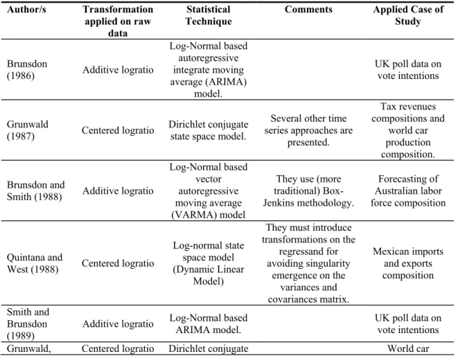
The following Table summarizes the previous reviews. There it can observed the respective paper reference, the transformation applied to raw data, the statistical technique, specific comments of the reviewer (if any), and the application field authors’ did for testing their models. As observed, alr and clr transformations were both applied in the different papers, the predominant statistical method is (variations of) state space modelling and most of the cases of study are from social sciences area.

Table 1. Summary of papers Author/s Transformation

applied on raw data

Statistical

Technique Comments Applied Case of Study

Brunsdon (1986) Additive logratio Log-Normal based autoregressive integrate moving average (ARIMA) model. UK poll data on vote intentions Grunwald (1987) Centered logratio Dirichlet conjugate state space model.

Several other time series approaches are

presented. Tax revenues compositions and world car production composition. Brunsdon and

Smith (1988) Additive logratio

Log-Normal based vector autoregressive moving average (VARMA) model

They use (more traditional) Box-Jenkins methodology. Forecasting of Australian labor force composition Quintana and

West (1988) Centered logratio

Log-normal state space model (Dynamic Linear

Model)

They must introduce transformations on the regressand for avoiding singularity emergence on the variances and covariances matrix. Mexican imports and exports composition Smith and Brunsdon (1989)

Additive logratio Log-Normal based _{ARIMA model.} UK poll data on _{vote intentions} Grunwald, Centered logratio Dirichlet conjugate World car

Raftery, and Guttorp (1993)

state space model production

composition. Cargnoni, Müller, and West (1995) Logratio Conditionally Gaussian dynamic model Forecasting of number and composition of secondary school students in Italy. Brandt, Monroe, and Williams (1999) Centered logratio Compositional Vector Autoregression (CVAR) system.

They deal with the same problem that Quintana and West (1988) and introduce analogous transformations on regressands. Socioeconomic and political determinants of Partisanship composition. Ravishanker, Dey, Iyengar (2004) Additive logistic Linear regression with (VARMA) errors and Hierarchical Bayesian selection model. Los Angeles mortality composition.

We finish the paper in the next section with the conclusions.

4. Conclusions

Throughout the review three main variables have been observed: the transformations, the statistical models, and the cases of study. For the first ones, additive and centered logratios have been equaled used for the scant literature. However, none of the papers have compared the efficiency or appropriateness of each of the transformations for the specific case of study or statistical modelling. We know that alr transformation is not isometric and the clr transformation is isometric but constrained4_{. As a good remark}

has to be noted that Quintana and West (1988) and Brandt, Monroe, and Williams (1999) have deal with the problems of clr-tranformation zero-sum constraint by exogenously modifying the regressands in the linear regression equation. Further studies are required, again, for the appropriateness of this ad-hoc solution.

Second, several statistical techniques have been quoted. Such diversity ironically points out the lack of any methodology conventionally applied for dealing with CTS. Traditional time series analysis has a stock of available techniques that has not been applied using transformations from compositional data analysis, for instance, error-correction models, panel data analysis (Baltagi, 1995), dynamic panel data (Arellano and Bond, 1991). While works that use VAR and ARIMA modelling procedures have been quoted, most of the literature relies on state space modelling variants that diverse degree of success have shown in dealing with constrained data. But for many social scientists this specific model usually is not study in regular courses of Statistics or Econometrics.

Finally, the majority of the motivational cases of study of these papers came from social sciences problems. This is paradoxical with the finding that only some of these statistical techniques are widely available for the average social scientist. We could argue the same in terms of the required transformation for solving the constant-sum constraint.

Dynamic compositional problems are of substantive interest for social sciences. Examples like the evolution of federal budgets components, tax revenues compositions, income distribution, savings and investment composition during periods of crisis, represent interesting issues for future analysis. We think that it is lacking the application of well known transformations into also well known least squares methods for widening the knowledge and understanding of these methods in time series social sciences research and teaching.

References

Abril, J.C. (1999). Análisis de series de tiempo basado en modelos de espacio de estado. Buenos Aires: EUDEBA. 215 p. (In Spanish).

Aitchison, J. (1986). The Statistical Analysis of Compositional Data. London, New York: Chapman and Hall. 417 p.

Aitchison, J. and S.M. Shen (1980). “Logistic-normal distribution: some properties and uses”. Biometrika 2 (67), 261-272.

Anderson, T.W. (1994). The Statistical Analysis of Time Series. John Wiley & Sons.

Arellano, M. and S. Bond (1991). “Some Tests of Specification for Panel Data: Monte Carlo Evidence and an Application to Employment Equations”. Review of Economic Studies 58, 277-294. Baltagi, B.H. (1995). Econometric Analysis of Panel Data. New York: John Wiley and Sons.

Brandt, P.T., B.L. Monroe, and J.T. Williams (1999). “Time Series Models for Compositional Data”. Unpublished paper. Department of Political Science. Indiana University, Bloomington.

Broemeling, L.D. and S. Shaarawy (1986). “A Bayesian Analysis of Time Series”. In P. Goel and A. Zellner (eds.). Bayesian Inference and Decision Techniques. Elsevier Science Publishers B.V. Brunsdon, T.M. (1986). Times series of compositional data. Ph.D. Thesis dissertation. University of

Southampton

Brunsdon, T.M. and T.M.F. Smith (1988). “The Time Series Analysis of Compositional Data”. Journal of Official Statistics 14 (3): 237-253.

Cargnoni, C., P. Müller, and M. West (1995). “Bayesian Forecasting of Multinomial Time Series through Conditionally Gaussian Dynamic Models”. Unpublished paper. Universitá di Firenze and Duke University.

Egozcue, J., V. Pawlowsky-Glahn, G. Mateu-Figueras, and C. Barceló-Vidal (2003). “Isometric Logratio Transformations for Compositional Data Analysis”. Mathematical Geology 35 (3): 279-300. Enders, W. (1995). Applied Econometric Time Series. Toronto: John Wiley & Sons. 433 p.

Grunwald, G.K. (1987). Time Series Models for Continuous Proportions. Ph.D. Thesis Dissertation. Department of Statistics. University of Washington. 104 p.

Grunwald, G.K., A.E. Raftery, and P. Guttorp (1993). “Time Series of Continuous Proportions”. Journal of the Royal Statistical Society, Series B 55 (1): 103-116.

Hamilton, W. (1994). Time Series Analysis. Princeton: Princeton University Press.

Harvey, A.C. (1989). Forecasting Structural Time Series Models and the Kalman Filter. Cambridge: Cambridge University Press.

Porier, D.J. and J.L. Tobias (2005). “Bayesian Econometrics”. Unpublished paper. Iowa State University. Quintana, J.M. and M. West (1988). “Time Series Analysis of Compositional Data”. In J.M. Bernardo,

M.H. DeGroot, D.V. Lindley and A.F.M. Smith (Eds.). Bayesian Statistics 3: 747-756.g

Ravishanker, N., D.K. Dey, and N. Iyengar (2004). “Compositional Time Series of Mortality Proportions”. Unpublished paper. Department of Statistics, University of Connecticut.

Sims, C. (1980). “Macroeconomics and Reality”. Econometrica 48 (1): 1-48.

Smith, T.M.F. and T.M. Brunsdon (1989). “The Time Series Analysis of Compositional Data”. Proceedings of the American Statistical Association: 1-12.

Theil, H. (1971). Principles of Econometrics. New York: Wiley.