www.elsevier.com/locate/camwa
Logic classification and feature selection for biomedical data
P. Bertolazzi
a,∗, G. Felici
a, P. Festa
b, G. Lancia
caIstituto di Analisi dei Sistemi ed Informatica “Antonio Ruberti” del CNR, Viale Manzoni 30, 00185, Rome, Italy bDipartimento di Matematica e Applicazioni “R.M. Caccioppoli”, Universit´a degli Studi di Napoli Federico II, Italy
cDipartimento di Informatica e Matematica, Universit´a di Udine, Italy
Abstract
In this paper we investigate logic classification and related feature selection algorithms for large biomedical data sets. When the data is in binary/logic form, the feature selection problem can be formulated as a Set Covering problem of very large dimensions, whose solution is computationally challenging. We propose an alternative approximated formulation for feature selection that results in an extension of Set Covering of compact size, and use the logic classifierLsquareto test its performances on two well-known data sets. An ad hoc metaheuristic of the GRASP type is used to solve efficiently the feature selection problem. A simple and effective method to convert rational data into logic data by interval mapping is also described. The computational results obtained are promising and the use of logic models, that can be easily understood and integrated with other domain knowledge, is one of the major strengths of this approach.
c
2007 Elsevier Ltd. All rights reserved.
Keywords:Logic data mining; Combinatorial feature selection; Set Covering
1. Introduction
In past years, research in molecular biology and molecular medicine has accumulated enormous amounts of data. Such large amount of information must be thoroughly analyzed to gain a better understanding of the underlying biological processes. Methods of knowledge discovery and data mining are the best candidates for this challenging task.
Important examples of large data sets are found in: (i) genomic sequences gathered by the Human Genome Project and sequences of Single Nucleotide Polymorphisms (SNPs); (ii) gene expression data from microarray experiments; (iii) protein identification and quantification data from proteomics experiments.
For each of these problems, different modeling, algorithmic, and interpretation problems arise (see [1–3] for presentation and discussion of fundamental issues and methodologies).
The study of both genomic sequences and SNP sequences is aimed at identifying the positions of base pairs responsible for function, mechanism or interaction. The analysis of SNPs permits us to understand the relationship
∗Corresponding author.
E-mail addresses:[email protected](P. Bertolazzi),[email protected](G. Felici),[email protected](P. Festa),[email protected]
(G. Lancia).
0898-1221/$ - see front matter c2007 Elsevier Ltd. All rights reserved.
between genotypic and phenotypic information, as well as to identify polymorphisms that can be related to specific genetic diseases. One application is the identification of gene/SNP patterns impacting cure/drug development for various diseases. Data sets are made of genomic or SNP sequences (in both cases, sequences of base pairs) of given individuals of the same species or of different but related species. The general analysis problem to be solved requires us to associate diversities and commonalities among individuals with differences and identities between their base pairs sequences.
Microarrays are semiconductor devices used to detect the DNA makeup of a cell. They contain hundreds of thousands of tiny squares, each designed to hybridize with a sequence encoding a particular gene. The microarray squares react to the liquified human cells poured over them, and capture the sequences that they are targeted to hybridize with. After the reaction, the amount of captured gene sequences is detectable by a laser, that reads the “expression” of each gene at the corresponding square. Microarrays are used, e.g., to identify drug targets (the proteins with which drugs actually interact) and can also help us to identify individuals with similar biological patterns. This way, drug companies can choose the most appropriate candidates for participating in clinical trials of new drugs. Data from microarray experiments are two-dimensional arrays, in which each entry corresponds to the expression of one specific gene. Given a set of arrays (experiments on the same microarray), the analysis problem is to classify the experiments, taking into account the value of gene expressions for a small number of genes.
Finally, data bases of proteins exist that contain primary, secondary, and tertiary structures of each protein. There are protein families with common properties, whose functions are characterized by patterns in their three-dimensional structure. Here one wants to detect subsets of amino acids of the chains that are linked to the analyzed properties. In particular, with each amino acid is associated the measure of the studied properties.
All these data sets are typically represented by matrices whose rows are associated with the objects, or records, while the columns are associated with the many measures taken on each object. Such measures are often referred to as variables, orfeatures. For the analysis of such type of data there are analysis tools with different degree of complexity, where the complexity is to be found in the models that are needed and in the large dimension of the data that are to be processed. Such techniques are being referred to asdata mining(DM), indicating a collection of methods inherited mainly from the classical multivariate and nonparametric statistics, the Computer Science oriented Learning Theory, mathematical programming, and Artificial Intelligence.
Data mining is used to systematically explore the possibility of relations between variables when there are no (or incomplete) a priori expectations as to the nature of those relations. Its use in biology and medicine has grown rapidly since 1997. When dealing with large data sets, it is often the case that the information available is somehow redundant for the scopes of the DM application; many mining tools deal with this issue by trying to provide classification or association rules that are as much compact as possible.
In conjunction with data mining techniques it is common to applyfeature selection(FS), by which we address a set of methods to identify, in a large set, those features that are best useful for the specific analysis task, be it the identification of a classification model, of association rules, or a statistical regression model. The role of feature selection is particularly important when computationally expensive data mining tools are used, or when the data collection process is difficult or costly, as it is the case in the type of applications that we consider here.
In this paper, we test the efficacy of a particular class of feature selection methods for classification on data sets represented in binary, or logic form, in conjunction with a method to mine logic relations in the data, theLsquare system (see [4,5]).Lsquaremodels the classification problem as a sequence of minimum cost satisfiability problems (MINSAT) and is able to find separating formulas optimized according to certain criteria. To reduce the intractable dimensions of the data sets analyzed, we consider FS methods based on another well-known combinatorial problem, the Set Covering Problem (SC). We propose a simplified version of such models that significantly reduces the dimension of the Set Covering problem to be solved showing that also in this case we are able to identify a good and small subset of the available features.
The paper is organized as follows.
Section2introduces the main issues in designing a FS method and the most basic and widely known techniques; then, describes the basic ideas of the Set Covering formulation, focusing both on the quadratic formulation already presented in [6], and on the simplified linear version proposed in this paper. A specific subsection deals with the complexity issues related with the solution of a large SC problem and describes the metaheuristic algorithm used to solve the large instances associated with FS. In Section3, the basic steps of theLsquaremethod for logic learning are presented. Then, Section4describes the techniques used to preprocess the data, in particular to obtain data in logic
form from measures expressed through real numbers, as it is the case for microarray data. Such a process, known as discretizationorbinarization, is not to be overlooked in the entire process as it accomplishes a relevant transformation of the available information and influences the work of FS and DM. Then, in Section 5we synthesize the whole analysis process, and report and discuss the experimental results obtained. Conclusions are drawn in Section6together with some consideration on future work in this challenging research area.
2. Feature selection methods
In many applications FS may be considered as an independent task in the mining process; it is used to reduce the data to a treatable size before it can be processed by a DM algorithm. A reason behind this strategy is that sophisticated DM algorithms often may fail, or have significant computational problems, when treating directly data set with a very large number of features, as in the case of biomedical data. A very extensive treatment of the use of FS in DM applications is given by Liu and Motoda [7], who provide a complete overview of the methods developed since the 70s, comparing the results of several applications and providing suggestions on how to drive the choice of the proper method for each specific problem. Feature selection problems are typically solved in the literature using search techniques, where the evaluation of a specific subset is accomplished by a proper function (filter methods), or directly by the performance of a data mining tool (wrapper methods). A general overview of different methods is also available in [8,9]. In this paper, we focus on data represented by binary features and try to exploit particular methods that are designed for such cases. As we will see later in Section4, our proposal is to convert, by proper binarizationtechniques, rational features into binary features in order to apply logic-based classification methods. Such a binarization process induces a further proliferation of the number of features, and thus demands even more strongly a valid method to reduce the size of the problem to a treatable one. In the following sections we describe such methods.
2.1. Feature selection for biological data analysis
Many FS methods have been applied in biological data analysis. Most of such work concerns microarrays classification, where the number of features is in the range of several thousands. In [10] the authors propose a hybrid of filter and wrapper approaches to feature selection, based on Unconditional Mixture Modeling, Information Gain Ranking, and Markov blanket Filtering. In [11,12] redundancy-based methods are applied. Support Vector Machines are used as a classification method to prove the goodness of a selected feature set in [13,14]. In [15], Nearest Neighbor methods and Support Vector Machines are used for predicting protein functional classes from binary vectors obtained by comparing functional domains in the SBASE database to each protein sequence. In [16] a global search mechanism, weighted decision tree, decision-tree-based wrapper, a correlation-based heuristic, and the identification of intersecting feature sets are employed for selecting significant genes/SNPs for predicting drug effectiveness. 2.2. Set Covering formulation for feature selection: The minimal test collection
When dealing with binary features, the problem of selecting a subset of features of minimal size that guarantees the separation between two sets can be formulated as an Integer Linear Programming Problem, more specifically as a Set Covering problem. Here we consider a known formulation, that suffers from the fact that its size, in terms of number of rows, increases quadratically with the number of rows of the data matrix.
A formal definition of the problem of feature selection (calledtest cover) is presented in [17]. The input is a set of items{1, . . . ,m}(e.g., arrays of gene expression from a microarray experiment) and a collectionFof features (e.g. a feature could be a gene){f1, . . . , fn}. The item set is divided into two classes, (e.g., microarrays obtained from DNA of sick patients and microarrays obtained from DNA of healthy ones). By convention, we indicate the two classes byclass Aandclass B, respectively. For each itemh, each feature fi takes a value in a given metric. In a binary setting each feature has two possible values{1,0}, representing the presence or the absence of a given characteristic, associated with that feature, in itemh. To represent the value of featureifor itemhwe use the notation fi h, that would then take value 0 or value 1. A feature fi differentiates (covers) item pair{k,h}if fi k 6= fi h. If we consider all the pairs of items{k,h}wherekbelongs to a class (say, “healthy patients”) andh belongs to the other class (say, “sick patients”), then a subcollectionF ⊂ Fof features is a cover if each of such pairs{k,h}is covered by at least one
element inF. Obviously, the number of pairs is equal to the product of the cardinalities of the two classes, that grows quadratically withm. The problem of finding a subset of features of minimal size that cover all the pairs of distinct elements is calledCombinatorial Feature Setorminimal test collection. A mathematical formulation of the problem is given below: min n X i=1 xi n X i=1 ai jxi ≥1 j =1. . .M xi ∈ {0,1} i =1. . .n, (1)
wherexi =1 if fi is chosen and 0 otherwise; each of the M constraints is associated with a pair of items belonging to different classes; e.g., if row j is associated with the item pair{k,h}then we have that for featurei ai j =1 if and only if fi k 6= fi h. Here we refer to the above problem as QSC (Quadratic Set Covering).
For the QSC problem, in [6] a branch-and-bound procedure is presented, based on a new definition of branching rules and lower bounds. Nevertheless, when problem size is significantly large, the use of optimization algorithms to produce guaranteed optimal solutions becomes impractical, and one has to resort to heuristics schemes, such as, among the others, the one proposed in [18]. The above approach to the FS problem presents also additional drawbacks. Its purpose is to find a minimal set that can separate the given data, that plays the role oftrainingdata in the general process. The features associated with the minimal set are then used to project the training data and to derive classification rules, that are then applied to testdata, once the latter has been projected using the same feature set. When the data is noisy or not well sampled, it may happen that the very thrifty representation of the data overlooks some features that, although not strictly needed for separating the training data, may play a role in formulas that behave well on testing data. In other words, maintaining a certain measure of redundancy in the information that is retained by the FS process may be a good strategy for the production of rules with good predictive power. This is particularly true when FS is followed by classification algorithms that can perform an additional selection of the features based on the separating model. For this reason, we want to evaluate the quality of the QSC formulation also when the requirement on the number of covering features is raised, that is when therhsof the covering constraints is greater than 1. This would result in the selection of a larger set that brings more information in the classification step. In the present setting, such modification is easy to make on the modeling side, as it is sufficient to rewrite the covering constraints of QSC as follows: min n X i=1 xi n X i=1 ai jxi ≥α j=1. . .M xi ∈ {0,1} i =1. . .n, (2)
whereαis an integer representing the degree of redundancy required. In such case, the standard Set Covering problem is transformed into a Generalized Set Covering (GSC) problem and many of the known results and algorithms cannot be applied in a straightforward fashion. To any extent, the QSC formulation is computationally very expensive to solve, and we propose a more compact model based on a GSC formulation that does not guarantee to find a subset of the features that perform perfect separation in the training set, but identifies a small set of highly informative and loosely correlated features. This is done with a consistently smaller computational effort as compared with that of QSC.
2.3. An approximated formulation of the feature selection: The “Linear” Set Covering
The approximated Set Covering formulation described in this section is based on a very simple idea. Given a feature fi, letPA(i)andPB(i)be the proportion of items where feature fi has value 1 in setsAandB, respectively. IfPA(i) >PB(i), then the presence of fi with value 1 is likely to characterize items that belong to A, and viceversa.
Let us assume that we are in this case, that is,PA(i) >PB(i), and define for fi the following vectordi j, j =1, ..,m (note that here j is used to refer a single item, and not a pair of items as in models(1)and(2)):
di j =
1, if item jis in classAand fi has value 1; 0, if item jis in classAand fi has value 0; 1, if item jis in classBand fi has value 0; 0, if item jis in classBand fi has value 1.
For the casePA(i) < PB(i), the corresponding vectorai j is computed in the same way by exchanging the roles of AandB. A feature fi withai j =1 for all j ∈1, ..,mwould be able to discriminate perfectly betweenAandB, as it would suffice to tell whether an item belongs to one of the two classes. Obviously, such a feature is not likely to exist, but we may assume that the number of ones in vectorai j is positively correlated with the discriminating power of feature fi. Moreover, we would like to select a subset of the features that exhibit, as a set, a good discriminating power for all the items considered, so that we may use more features combined together, among the ones in the set, to obtain a complete separation between AandB. According to this line of reasoning, we formulate the following Set Covering problem: min n X i=1 xi n X i=1 di jxi ≥α j =1. . .m xi ∈ {0,1} i =1. . .n, (3)
where, as in QSC,xi =1 implies that feature fi is selected in the final set andαrepresents the degree of redundancy of the information provided by the selected features. Although such formulation does not guarantee exact separation, it identifies good features that exhibit their discriminating power in a distributed way over the item set, due to the presence of the samerhsαfor each item. The problem above is referred to as LSC (Linear Set Covering) and has the same nature as QSC but only a linear number of constraints. Some of the results conducted on large data sets show experimentally that the trade-off between the approximation of the LSC model and its computational simplicity may be worth considering.
In the above QSC and LSC formulations we have presented very trivial objective functions, that simply minimize the size of the feature sets. It is important to note that both models are designed to host additional information by means of proper weights associated with the features, that can be taken into account to drive the solution algorithm towards the choice of particular features, according to contextual consideration. For example, we may want to drive the algorithm towards particular features that, a priori, have a special role in the genetic phenomenon under study; or we may choose the weights in such a way that those features associated with the extremes of the measuring scale of a gene expression in microarray data are preferred as they are less prone to measuring errors.
2.4. GRASP heuristic
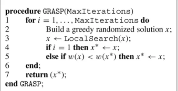
To solve the generalized Set Covering problems we pursue a non-deterministic and heuristic method known in the literature as GRASP, acronym of Greedy Randomized Adaptive Search Procedure. GRASP is a randomized multistart iterative metaheuristic initially proposed in Feo and Resende [19,20]. For a comprehensive study of GRASP strategies and variants, the reader is referred to the survey chapter by Resende and Ribeiro [21], as well as to the annotated bibliography of Festa and Resende [22] for a survey of applications. Generally speaking, GRASP is a randomized heuristic having two phases: a construction phase and a local search phase. The construction phase adds one element at a time to a set that ends up with a representation of a feasible solution. At each iteration, an element is randomly selected from arestricted candidate listRCL, whose elements are among the best ordered, according to some greedy function. Once a feasible solution is obtained, the local search procedure attempts to improve it by producing a locally optimal solution with respect to some neighborhood structure. The construction and the local search phases are repeatedly applied. The best solution found is returned as an approximation of the optimal one.Fig. 1depicts the pseudo-code of a generic GRASP heuristic for a minimization problem.
Fig. 1. Pseudo-code of a generic GRASP for a minimization problem.
The construction phase makes use of an adaptive greedy function, a construction mechanism for the restricted candidate list, and a probabilistic selection criterion. The greedy function takes into account the contribution to the objective function achieved by selecting a particular element. In the case of the generalized unweighted Set Cover problem, the selection involves candidate features and it is intuitive to relate the greedy function to the number of constraints still to be fully covered that a feature not yet chosen would cover if selected. More formally, at a generic iteration of the GRASP construction phase letF⊂Fbe the subset of features already selected as the partial solution and letC⊆Cbe the subset of constraints still to be fully covered. Then, for each f ∈F\Fwe defineσ(f)= |Cf|, whereCf ⊆ C is the subset of constraints not yet fully covered that feature f would cover. This greedy function measures how much additional cover will result from the selection of f. The greedy choice consists in selecting the feature f ∈ F \F with the highest greedy function value. To define the construction mechanism for the restricted candidate list RCL, let
σmin=min{σ(f)| f ∈ F\F} and
σmax=max{σ(f)| f ∈F\F}. (4)
Denoting byµ=σmin+β·(σmax−σmin)the cut-off value, whereβis a parameter such that 0≤β ≤1, the restricted candidate list RCL is made up by all features whose value of the greedy function is greater than or equal toµ. A feature is randomly selected from the restricted candidate list and the setsFandCare updated accordingly to the just made selection (adaptive component).
Since we are dealing with the problem in its unweighted variant, the local search procedure only checks for redundancy of the current solution built by the GRASP construction phase, which is replaced by its best improving neighbor. The search stops after all possible moves have been evaluated and no improving neighbor has been found. 3. The learning systemLsquare
The learning tool used in this application,Lsquare, is a particular learning method that operates on data represented by logic variables and produces rules in propositional logic that classify the items in one of two classes. The general scheme of this method is the one of automatic learning, where the items presented in atraining setare used to infer the rules that link the class of an item with the value of some of its features; these rules are then used to classify new records and predict their class.
The choice ofLsquareis motivated by the fact that it uses a logic representation of the description variables, that are to all extents logic variables, and of the classification rules, that are logic formulas in Disjunctive Normal From (DNF). Such property enables us to analyze and interpret the classification results also from the semantic point of view, as the classification rules determined by the method express combination of the features that can be interpreted by domain experts and bring to light new knowledge in an easily understandable format.
The learning of propositional formulas from data is tackled also by other learning methods, such as the strongly heuristic, simple and widely used decision trees (originally proposed in [23]), to the more sophisticated LAD system, originally proposed by Hammer in [24,25], with complexity and mathematical programming issues similar to those faced inLsquare, to the greedy approach proposed in [26].
TheLsquaresystem and some of its additional components have been described in other papers [4,27,5] and its detailed description is out of the scope of this paper. Here, we simply mention the fact that the rules are determined using a particular problem formulation that amounts to be a well-known and hard combinatorial optimization problem, the minimum cost satisfiability problem, or MINSAT, that is solved using a very sophisticated solver based on decomposition and learning techniques [5]. The DNF formulas identified have the property of being created by conjunctive clauses that are searched for in order of coverage of the training set. Therefore, they usually are formed by few clauses with large coverage (the interpretation of the trends present in the data) and several clauses with smaller coverage (the interpretation of the outliers).
4. Preprocessing and data binarization
The preprocessing phase was conceived to transform input data from a problem dependent format to a problem independent format. In general, biological data sets are large arrays of integers or real numbers, that correspond to measures on the items. Such data are not suitable for logic methods, and a transformation is needed to adapt the data sets. This transformation consists of the identification of a set of intervals of values for each feature, the computation of the number of samples in each interval, and a reduction of the number of these intervals through the elimination of empty intervals and unification of contiguous intervals with the same meaning. In binarized data, the new features can be viewed as binary, or logic, variables, that indicate whether the measure of one of the original real features belongs to a certain interval.
To obtain an initial set of intervals for feature fi we consider its meanµi and varianceσi over the training items, and create a number of equal sized intervals symmetrical with respect toµand proportional in size toσi. Once such intervals have been created, we iterate a set of steps that merge two adjacent classes if one of them is empty, if the proportion of elements inAandB is not altered when the two classes are merged (class entropy), and finally if the reduction obtained in the entropy of the feature is negligible.
For a given feature fi, let Ki be the set of the intervals in which fi is discretized; its entropyhi is given by −P
k∈Ki fi klog fi k, where flk =plk/n, and plkis the number of samples included in the intervalk; sincehi =0 if
the number of intervalsKi is equal to 1, the goal is to obtain a good trade-off between a high level of entropy and a small number of intervals. The procedure performs the following steps on the training data set:
1. for each feature fi, the mean valueµiand the varianceσi of the values of the feature over the items of the training set are evaluated;
2. Nintervals aroundmi are computed, so that each interval widthwiis equal to √
σi/N(such intervals are indicated withCi k, fork=1, ..,N);
3. for each intervalCi k, the total numberpi kof samples that are included in the interval is determined, together with the number of samples that are in classA,pi kAand the number of samples that are in class B,pi kB.
4. The Nintervals are reduced on the basis of the following three criteria:
• if an interval is empty then it is unified with one of the smaller of its adjacent intervals;
• if in two adjacent intervals class A(B) samples are strongly prevalent over those of B (A) samples, the two intervals are unified;
• if one interval is poorly populated it is unified with one of the two adjacent classes if the entropy level of the feature does not fall below a given threshold.
Given the final set of intervals, a binary representation of the values of the feature is obtained by mapping the rational value of that feature into its corresponding interval, and setting the corresponding binary variable to 1. 5. Experiments and results
We have applied the classification procedures described above to two data sets characterized by a very large number of features, that have already been considered in other similar works. Such choice is driven by the intention to test the efficacy of the methods for problems in this application area, in order to gain the sufficient thrust to apply them in real problems where the results may be of some potential interest. The experiments described below have the same structure: atrainingset of data is analyzed with the FS Set Covering models to extract a significant and small subset of the features; then,Lsquareis applied to extract a logic model that separates at best the two setsAandBwith the
Table 1
Thrombin data set: Correct recognition rate for 50% split testing with LSC FS and increasing value ofα
Values ofα % correct onA % correct onB Total correct
10 0.673 0.399 0.426 20 0.629 0.617 0.618 30 0.588 0.757 0.740 40 0.609 0.790 0.772 50 0.622 0.829 0.809 60 0.622 0.822 0.803 70 0.620 0.858 0.835 80 0.620 0.857 0.834
available features. Finally, such a model is applied ontestdata, i.e., data of the same nature of the training set, for which we know the classification in AandB, but that has not been considered in the training phase. The percentage of correct recognition on thetestset is a reasonable measure of the quality of the whole method, and can be compared with other ones already presented in the literature. According to the purpose of the paper, we investigate the behavior of the performances of the system when the main experimental parameters are varied.
In Section 5.1, we describe the experiments conducted on the thrombin data set. Here no preprocessing and binarization is needed, as the data has been already made available in binary form. The problem is of large size and we were able to solve the QSC problem optimally and with the proposed heuristic procedure, and compare its results with those obtained with the LSC feature selection method.
In Section5.2, we consider a typical case of classification of microarray data where the genes should differentiate between patients with two different types of leukemia. Here the whole process is tested, including the binarization. The behavior of the LSC and QSC models with different values ofαis analyzed.
5.1. Thrombin data set
Thrombin data set was extracted from KDD competition [28] for testing the performances of various procedures for data mining. The problem of analyzing the molecular bioactivity of drugs w.r.t. a receptor, in order to separate the active (binding) compounds from the inactive (non-binding) ones was proposed. The data set1includes compounds that binds to thrombin, a key receptor in blood clotting, and compounds that do not bind. The problem was to identify a small set of sites of the compound molecules that allow us to separate active vs inactive compounds. Two sets of data are provided: the training data set includes 1909 known molecules (42 actively binding thrombin), the test data set includes 639 new compounds with unknown capacity to bind thrombin; 139.351 binary features describe the three-dimensional properties of each compound. The chemical structures of these compounds are not relevant for our analysis and are not included. The definitions of the individual bits are not included — we do not know what each individual bit means, only that they are generated in an internally consistent manner for all compounds. Thrombin data set was not preprocessed since it is a binary data set and was used straightforwardly to generate the LSC problem. The performance of our method is compared with the Jie Cheng method, the winner of the KDD cup 01 [28], that used a Bayesian network predictive model.
Table 1reports the results obtained when the LSC method is used, for values ofαranging from 10 to 80. Each experiment is obtained by a 50% random split of the available data into training and testing, repeated 8 times and then averaged. The level of the recognition percentages is comparable with those characterizing the best results obtained on the same data available in the literature [28], when the value ofα reaches 80. The best formulas obtained use approximately 60 features, and it explains why the good results are obtained whenαreaches that value.
It is of some interest to compare the results ofTable 1with those obtained using a subset of features selected by the optimal solution of the associated QSC. Such solutions have been obtained at an unpractical computational cost by a Branch & Cut algorithm that uses the latest version of the ILOG Cplex solver for integer programming. The minimal test is composed of only 41 features, but the performances measured with the same metric are significantly worse than the ones obtained with LSC. Moreover, the optimal solution of 41 features is not unique, and the many solutions of that
Table 2
Leukemia data set: Correct recognition rate and solution dimensions for testing set with LSC FS and increasing value ofα
Values ofα Dimensions of features set Used features Correct onA Correct onB Total correct
1 2 1 0.900 0.500 0.735 2 3 3 0.950 0.500 0.765 3 5 4 1.000 0.643 0.853 4 6 3 0.700 0.571 0.647 5 7 3 0.850 0.857 0.853 10 14 4 0.950 0.643 0.824 15 20 3 0.950 0.714 0.853 20 26 2 0.900 0.929 0.912 30 39 3 0.900 0.643 0.794 35 46 2 0.900 0.929 0.912 65 85 2 0.900 0.929 0.912 75 97 2 0.900 0.929 0.912 Table 3
Leukemia data set: Correct recognition rate and solution dimensions for testing set with QSC FS and increasing value ofα
Values ofα Dimensions of features set Used features Correct onA Correct onB Total correct
1 2 2 0.650 0.643 0.647 2 4 2 0.850 0.929 0.882 3 6 2 0.850 0.429 0.676 4 7 3 1.000 0.357 0.735 5 9 2 0.950 0.500 0.765 10 17 3 0.850 0.929 0.882 15 23 3 0.850 0.929 0.882 30 31 2 0.850 0.571 0.735 35 49 2 0.900 0.286 0.647 50 58 3 1.000 0.214 0.676 65 75 2 0.900 0.929 0.912
dimension show high variances in their performances. It so appears that better FS solutions are obtained by enforcing a significant level of redundancy in the information retained by the selected features, devolving to the classification algorithm (Lsquare, in this case) the task of selecting a good separating model and the features that support it. 5.2. Leukemia data set
The other data set was derived from microarray experiments. It is a collection of 72 samples from leukemia patients; each sample gives the expression level of 7130 genes [29]. The collection includes 47 samples from type I leukemias (called AL L) and 25 from type II leukemias (called AM L). The collection is split into two sets, the first with 38 samples(AL L/AM L =27/11)serving as a training set, and the other 34(20/14)as a test set. Here, we deployed also the preprocessing and the binarization stage. Each feature was initially divided into intervals with high granularity (according to the scheme described in Section4). From each feature we derived 30 intervals, obtaining 213,900 initial features, that were then reduced to approximately 120,000 using the proposed procedure. Such a still large set of features were used to build the formulation of the LSC and QSC, that were then solved with different values ofα. A synthesis of the results obtained is given inTables 2and3, where we report the values ofα, the correct recognition percentages, the size of the feature set selected by the solution of the LSC and QSC models respectively, and also the number of features effectively used by the classification algorithm to build the separating logic model.
Comparing the two tables, it is easy to see that the LSC model performs as good as the QSC one, at times even better, although computationally less expensive. But the very interesting result in this case is that, besides having recognition percentages that match in quality with those obtained by many other methods presented in the literature [10], the size of the good formulas obtained is very small, usually composed of only 2 features, regardless of the dimension of the set of features selected by the solution of LSC/QSC. This implies that we can indicate not only the two genes that seem to differentiate the two types of leukemia, but also the levels at which such genes should
express in order to be significant. For example, if we consider one of the separating formulas obtained on 2 features, we may “translate” it into its original values and describe it as follows:
IF the expression of gene in position 5 is less than −429.99
OR larger than −420.77
AND the expression of gene in position 6 is below −148.1325
THEN the item is of type ALL, ELSE is of type AML.
Obviously such a statement may lack significance for a geneticist, but its compactness surely makes it understandable and potentially interesting from the semantic point of view. We recall that the rule above is able to separate exactly the observations in the training set, while it achieves an overall precision of 0.922 on provided testing data.
6. Conclusions
In this work, an approach for the solution of classification problems in data sets with a large number of features has been presented. The method is based on the representation of data in binary/logic form; when the data is not naturally available in this form, discretization procedures as the one presented in Section4of this paper can be used. The feature selection step is the main focus of the paper. We propose an alternative and more compact formulation as a Generalized Set Covering (where therhsmay assume values larger than 1) and solve it using a GRASP metaheuristic for the quite large data sets used for the experiments. The results obtained show that the method has some potential and its simplicity does not seem to affect the quality of the results. Additional considerations have to be drawn as conclusive remarks to the work done.
First, we note that the computationally challenging Set Covering formulation, known also as the minimal test collection, does not always produce guaranteed quality feature subsets. The objective of minimizing the number of features that guarantee separability may give results too strict, and produce solutions that completely overlook certain aspects of the data that are useful for predictive and interpretative purposes. Some degree of redundancy may come in use, as proposed and experimentally validated in this paper. Moreover, the simpler and lighter formulation here presented as LSC turns out to be experimentally effective and more robust.
Second, the use of mathematical formulations as(1) and(3)allows the use of costs associated with features in the objective function. Such costs may very well represent prior knowledge of domain experts, and could be used to drive the solution towards those features that are more interesting or significant in the particular application. Another interesting aspect in the use of costs with binarized data is that they can be used to mitigate the effect of noise in the data, by assigning higher costs to those features that are associated with intervals close to the center of the measuring scale of the original numeric feature, and smaller costs to those with extreme values. In this way, the solution would tend to use features whose binary value is less affected by measuring errors and noise.
Last but not the least, the approach presented is strongly characterized by the representation of both data and separating model in logic form. This implies that the knowledge extracted from the data is easier to understand, to combine with previously existing knowledge, and to interact with, for domain experts. In our opinion, such a characteristic is extremely important in a research field where the previous experience has to be combined with knowledge extracted directly from data, and where the results of a mathematical/algorithmic tool have to be understood and validated ex post before they may be transferred to real applications.
References
[1] A. Tramontano, The Ten Most Wanted Solutions in Protein Bioinformatics, in: Mathematical Biology and Medicine Series, Chapman Hall/CRC Press, UK, 2005.
[2] D.B. Allison, G.P. Page, T.M. Beasley, J.W. Edwards (Eds.), DNA Microarrays and Related Genomic Techniques, in: Biostatistics Book Series, Chapman Hall/CRC Press, UK, 2005.
[3] Pui-Yan Kwok (Ed.), Single Nucleotide Polymorphism: Methods and Protocols, in: Methods in Molecular Biology, Human Press Inc, Totowa, New Jersey, 2003.
[4] G. Felici, K. Truemper, A minsat approach for learning in logic domains, INFORMS Journal on Computing 13 (3) (2001) 1–17. [5] K. Truemper, Design of Logic-Based Intelligent Systems, Wiley-Interscience, New York, 2004.
[6] M.J. De Bontridder Koen, B.J. Lageweg, J.K. Lenstra, J.B. Orlin, L. Stougie, Branch-and-bound algorithms for the test cover problem, in: ESA 2002: 10th Annual European Symposium on Algorithms, in: Lecture Notes in Computer Science, Springer, Berlin, 2002, pp. 737–742.
[7] H. Liu, H. Motoda, Feature Selection for Knowledge Discovery and Data Mining, Kluwer Academic Publishers, 2000.
[8] P. Langley, Selection of relevant features in machine learning, in: Proceedings of the AAAI Fall Symposium on Relevance, AAAI Press, 1994, pp. 140–144.
[9] V. De Angelis, G. Felici, G. Mancinelli, Feature selection for data mining, in: E. Triantaphyllou, G. Felici (Eds.), Data Mining and Knowledge Discovery Approaches Based on Rule Induction Techniques, Springer Massive Computing, 2006, pp. 227–252.
[10] E.P. Xing, M.I. Jordan, R.M. Karp, Feature selection for high-dimensional genomic microarray data, in: Proc. 18th International Conf. on Machine Learning, Morgan Kaufmann, San Francisco, CA, 2001, pp. 601–608.
[11] C. Ding, H. Peng, Minimum redundancy feature selection from microarray gene expression data, in: CSB ’03: Proceedings of the IEEE Computer Society Conference on Bioinformatics, IEEE Computer Society, Washington, DC, USA, 2003.
[12] L. Yu, H. Liu, Redundancy based feature selection for microarray data, in: KDD ’04: Proceedings of the Tenth ACM SIGKDD International Conference on Knowledge Discovery and Data Mining, ACM Press, 2004, pp. 737–742.
[13] D.A. Peterson, M.H. Tahut, Model and feature selection in microarray classification, in: IEEE Symposium on Computational Intelligence in Bioinformatics and Computational Biology, 2004, pp. 56–60.
[14] M.L. Chow, E.J. Moler, I.S. Mian, Identifying marker genes in transcription profiling data using a mixture of feature relevance experts, Physiological Genomics 5 (2001) 99–111.
[15] Y. Cai, A.J. Doig, Prediction of saccharomyces cerevisae protein functional class from functional domain composition, Bioinformatics 20 (8) (2004) 1292–1300.
[16] S.C. Shah, A. Kusiak, Data mining and genetic algorithm based gene/snp selection, Artificial Intelligence in Medicine 31 (3) (2004) 183–196. [17] M.R. Garey, D.S. Johnson, Computer and Intractability: A Guide to the Theory of NP- Completeness, Freeman, San Francisco, 1979. [18] P. Bonizzoni, G. Lancia, R. Rizzi, A practical approach to the healthy versus diseased minimal test collection problem when the tests are
powerful, manuscript, 2005.
[19] T.A. Feo, M.G.C. Resende, A probabilistic heuristic for a computationally difficult set covering problem, Operations Research Letters 8 (1989) 67–71.
[20] T.A. Feo, M.G.C. Resende, Greedy randomized adaptive search procedures, Journal of Global Optimization 6 (1995) 109–133.
[21] M.G.C. Resende, C.C. Ribeiro, Greedy randomized adaptive search procedures, in: F. Glover, G. Kochenberger (Eds.), State-of-the-Art Handbook of Metaheuristics, Kluwer, 2002, pp. 219–249.
[22] P. Festa, M.G.C. Resende, Grasp: An annotated bibliography, in: C.C. Ribeiro, P. Hansen (Eds.), Essays and Surveys on Metaheuristics, Kluwer Academic Publishers, 2002, pp. 325–367.
[23] Breiman, Friedman, Olshen, Stone, Classification & Regression Trees, Wadsworth, Pacific Grove, 1984.
[24] E. Boros, T. Ibaraki, K. Makino, Logical analysis of binary data with missing bits, Artificial Intelligence 107 (1999) 219–263.
[25] E. Boros, T. Ibaraki, A. Kogan, E. Mayoraz, I. Muchnik, An implementation of logical analysis of data, RUTCOR Research Report, Rutgers University, NJ, 1996, pp. 29–96.
[26] E. Triantaphyllou, A.L. Soyster, On the minimum number of logical clauses which can be inferred from examples, Computers and Operations Research 23 (1996) 783–799.
[27] G. Felici, K. Truemper, The Lsquare System for Mining Logic Data, in: J. Wang (Ed.), Encyclopedia of Data Warehousing and Mining, vol. 2, Idea Group Inc., 2006, pp. 693–697.
[28] C. Hatzis, D. Page, Kdd-2001 cup: The genomics challenge,http://www.cs.wisc.edu/dpage/kddcup2001/, 2001.
[29] T.R. Golub, D.K. Slonim, P. Tamayo, C. Huard, M. Gaasenbeek, J.P. Mesirov, H. Coller, M.L. Loh, J.R. Downing, M.A. Caligiuri, C.D. Bloomeld, E.S. Lander, Molecular classification of cancer: Class discovery and class prediction by gene expression monitoring, Science 286 (1999) 531–537.