Sparse model identification and learning for ultra-high-dimensional additive partially linear models

2019

Sparse model identification and learning for

ultra-high-dimensional additive partially linear models

Xinyi Li

University of North Carolina at Chapel Hill

Li Wang

Iowa State University, [email protected]

Dan Nettleton

Iowa State University, [email protected]

Follow this and additional works at:

https://lib.dr.iastate.edu/stat_las_pubs

Part of the

Multivariate Analysis Commons, and the

Statistical Models Commons

The complete bibliographic information for this item can be found at

https://lib.dr.iastate.edu/

stat_las_pubs/248. For information on how to cite this item, please visit

http://lib.dr.iastate.edu/

howtocite.html.

This Article is brought to you for free and open access by the Statistics at Iowa State University Digital Repository. It has been accepted for inclusion in Statistics Publications by an authorized administrator of Iowa State University Digital Repository. For more information, please contact

additive partially linear models

The additive partially linear model (APLM) combines the flexibility of nonparametric regression with the parsimony of regression models, and has been widely used as a popular tool in multivariate nonparametric regression to alleviate the “curse of dimensionality”. A natural question raised in practice is the choice of structure in the nonparametric part, i.e., whether the continuous covariates enter into the model in linear or nonparametric form. In this paper, we present a comprehensive framework for simultaneous sparse model identification and learning for ultra-high-dimensional APLMs where both the linear and nonparametric components are possibly larger than the sample size. We propose a fast and efficient two-stage procedure. In the first stage, we decompose the nonparametric functions into a linear part and a nonlinear part. The nonlinear functions are approximated by constant spline bases, and a triple penalization procedure is proposed to select nonzero components using adaptive group LASSO. In the second stage, we refit data with selected covariates using higher order polynomial splines, and apply spline-backfitted local-linear smoothing to obtain asymptotic normality for the estimators. The procedure is shown to be consistent for model structure identification. It can identify zero, linear, and nonlinear components correctly and efficiently. Inference can be made on both linear coefficients and nonparametric functions. We conduct simulation studies to evaluate the performance of the method and apply the proposed method to a dataset on the Shoot Apical Meristem (SAM) of maize genotypes for illustration.

Keywords

Dimension reduction, Inference for ultra-high-dimensional data, Semiparametric regression, Spline-backfitted local polynomial, Structure identification, Variable selection

Disciplines

Multivariate Analysis | Statistical Models

Comments

This is a manuscript of an article published as Li, Xinyi, Li Wang, and Dan Nettleton. "Sparse model

identification and learning for ultra-high-dimensional additive partially linear models."Journal of Multivariate Analysis173 (2019): 204-228. doi:10.1016/j.jmva.2019.02.010. Posted with permission.

Ultra-high-dimensional Additive Partially Linear Models

Xinyi Lia, Li Wangb and Dan Nettletonb

a_{SAMSI / University of North Carolina at Chapel Hill and}b_{Iowa State University}

Abstract: The additive partially linear model (APLM) combines the flexibility of nonparametric regression with the parsimony of regression models, and has been widely used as a popular tool in multivariate nonparametric regression to alleviate the “curse of dimensionality”. A natural question raised in practice is the choice of structure in the nonparametric part, that is, whether the continuous covariates enter into the model in linear or nonparametric form. In this paper, we present a comprehensive framework for simultaneous sparse model identification and learning for ultra-high-dimensional APLMs where both the linear and nonparametric components are possibly larger than the sample size. We propose a fast and efficient two-stage procedure. In the first stage, we decompose the nonparametric functions into a linear part and a nonlinear part. The nonlinear functions are approximated by constant spline bases, and a triple penalization procedure is proposed to select nonzero components using adaptive group LASSO. In the second stage, we refit data with selected covariates using higher order polynomial splines, and apply spline-backfitted local-linear smoothing to obtain asymptotic normality for the estimators. The procedure is shown to be consistent for model structure identification. It can identify zero, linear, and nonlinear components correctly and efficiently. Inference can be made on both linear coefficients and nonparametric functions. We conduct simulation studies to evaluate the performance of the method and apply the proposed method to a dataset on the Shoot Apical Meristem (SAM) of maize genotypes for illustration.

Key words and phrases: Dimension reduction, inference for ultra-high-dimensional data, semipara-metric regression, spline-backfitted local polynomial, structure identification, variable selection.

1

Introduction

In the past three decades, flexible and parsimonious additive partially linear models (APLMs) have been extensively studied and widely used in many statistical applications, including biol-ogy, econometrics, engineering, and social science. Examples of recent work on APLMs include Liang et al. (2008), Liu et al. (2011), Ma and Yang (2011), Wang et al. (2011), Ma et al. (2013), Wang et al. (2014) and Lian et al. (2014). APLMs are natural extensions of classical

Address for correspondence: Li Wang, Department of Statistics and the Statistical Laboratory, Iowa State University, Ames, IA, USA. Email: [email protected]

parametric models with good interpretability and are becoming more and more popular in data analysis.

Suppose we observe {(Yi,Z(i), X(i))}ni=1. For subject i = 1, . . . , n, Yi is a univariate

re-sponse, Z_(i) = (Zi1, . . . , Zip1)

> _{is a p}

1-dimensional vector of covariates that may be linearly associated with the response, andX_(i)= (Xi1, . . . , Xip2)

>_{is ap}

2-dimensional vector of contin-uous covariates that may have nonlinear associations with the response. We assume{(Yi,Z(i),

X(i))}ni=1 is an i.i.d sample from the distribution of (Y,Z,X), satisfying the following model:

Yi =µ+Z>_(i)α+ p2 X `=1 φ`(Xi`) +εi =µ+ p1 X k=1 Zikαk+ p2 X `=1 φ`(Xi`) +εi, (1)

whereµ is the intercept,αk,k= 1, . . . , p1, are unknown regression coefficients,{φ`(·)}p<sub>`=1</sub>2 are

unknown smooth functions, and each φ`(·) is centered with Eφ`(Xi`) = 0 to make model (1)

identifiable. The X(i) is ap2-dimensional vector of zero-mean covariates having density with a compact support. Without loss of generality, we assume that each covariate {Xi`}p`=12 can be rescaled into an interval χ = [a, b]. The εi terms are iid random errors with mean zero and

varianceσ2.

The APLM is particularly convenient whenZis a vector of categorical or discrete variables, and in this case, the components ofZenter the linear part of model (1) automatically, and the continuous variables usually enter the model nonparametrically. In practice, we might have reasons to believe that some of the continuous variables should enter the model linearly rather than nonparametrically. A natural question is how to determine which continuous covariates have a linear effect and which continuous covariates have a nonlinear effect. If the choice of linear components is correctly specified, then the biases in the estimation of these components are eliminated and root-nconvergence rates can be obtained for the linear coefficients. However, such prior knowledge is rarely available, especially when the number of covariates is large. Thus, structure identification, or linear and nonlinear detection, is an important step in the process of building an APLM from high-dimensional data.

When the number of covariates in the model is fixed, structure identification in additive models (AMs) has been studied in the literature. Zhang et al. (2011) proposed a penaliza-tion procedure to identify the linear components in AMs in the context of smoothing splines ANOVA. They demonstrated the consistency of the model structure identification and estab-lished the convergence rate of the proposed method specifically under the tensor product design. Huang et al. (2012b) proposed another penalized semiparametric regression approach using a group minimax concave penalty to identify the covariates with linear effects. They showed consistency in determining the linear and nonlinear structure in covariates, and obtained the convergence rate of nonlinear function estimators and asymptotic properties of linear coefficient

estimators; but they did not perform variable selection at the same time.

For high-dimensional AMs, Lian et al. (2015) proposed a double penalization procedure to distinguish covariates that enter the nonparametric and parametric parts and to identify significant covariates simultaneously. They demonstrated the consistency of the model struc-ture identification, and established the convergence rate of nonlinear function estimators and asymptotic normality of linear coefficient estimators. Despite the nice theoretical properties, their method heavily relies on the local quadratic approximation in Fan and Li (2001), which is incapable of producing naturally sparse estimates. In addition, employing the local quadratic approximation can be extremely expensive because it requires the repeated factorization of large matrices, which becomes infeasible when the number of covariates is very large.

Note that all the aforementioned papers (Huang et al., 2012b; Lian et al., 2015; Zhang et al., 2011) about structure identification focus on the AM with continuous explanatory variables. However, in many applications, a canonical partitioning of the variables exists. In particular, if there are categorical or discrete explanatory variables, as in the case of the SAM data studies (see the details in Section 5) and in many genome-wide association studies, we may want to keep discrete explanatory variables separate from the other design variables and let discrete variables enter the linear part of the model directly. In addition, if there is some prior knowledge of certain parametric forms for some specific covariates, such as a linear form, we may lose efficiency if we simply model all the covariates nonparametrically.

The above practical and theoretical concerns motivate our further investigation of the si-multaneous variable selection and structure selection problem for flexible and parsimonious APLMs, in which the features of the data suitable for parametric modeling are modeled para-metrically and nonparametric components are used only where needed. We consider the setting where both the dimension of the linear components and the dimension of nonlinear components is ultra-high. We propose an efficient and stable penalization procedure for simultaneously identifying linear and nonlinear components, removing insignificant predictors, and estimat-ing the remainestimat-ing linear and nonlinear components. We prove the proposed Sparse Model

Identification, Learning and Estimation (referred to as SMILE) procedure is consistent. We propose an iterative group coordinate descent approach to solve the penalized minimization problem efficiently. Our algorithm is very easy to implement because it only involves simple arithmetic operations with no complicated numerical optimization steps, matrix factorizations, or inversions. In one simulation example withn= 500 and p1 =p2 = 5000, it takes less than one minute to complete the entire model identification and variable selection process on a regular PC.

After variable selection and structure detection, we would like to provide an inferential tool for the linear and nonparametric components. The spline method is fast and easy to

implement; however, the rate of convergence is only established in mean squares sense, and there is no asymptotic distribution or uniform convergence, so no measures of confidence can be assigned to the estimators. In this paper, we propose a two-step spline-backfitted local-linear smoothing (SBLL) procedure for APLM estimation, model selection and simultaneous inference for all the components. In the first stage, we approximate the nonparametric functions φ`(·),

` = 1, . . . , p2, with undersmoothed constant spline functions. We perform model selection

for the APLM using a triple penalized procedure to select important variables and identify the linear vs. nonlinear structure for the continuous covariates, which is crucial to obtain efficient estimators for the non-zero components. We show that the proposed model selection and structure identification for both parametric and nonparametric terms are consistent, and the estimators of the nonzero linear coefficients and nonzero nonparametric functions are both

L2-norm consistent. In the second stage, we refit the data with covariates selected in the first step using higher-order polynomial splines to achieve root-nconsistency of the coefficient estimators in the linear part, and apply a one-step local-linear backfitting to the projected nonparametric components obtained from the refitting. Asymptotic normality for both linear coefficient estimators and nonlinear component estimators, as well as simultaneous confidence bands (SCBs) for all nonparametric components, are provided.

The rest of the paper is organized as follows. In Section 2, we describe the first-stage spline smoothing and propose a triple penalized regularization method for simultaneous model iden-tification and variable selection. The theoretical properties of selection consistency and rates of convergence for the coefficient estimators and nonparametric estimators are developed. Sec-tion 3 introduces the spline-backfitted local-linear estimators and SCBs for the nonparametric components. The performance of the estimators is assessed by simulations in Section 4 and illustrated by application to the SAM data in Section 5. Some concluding remarks are given in Section 6. Section A of the online Supplemental Materials evaluates the effect of differ-ent smoothing parameters on the performance of the proposed method. Technical details are provided in Section B of the Supplemental Materials.

2

Methodology

2.1 Model Setup

In the following, the functional form (linear vs. nonlinear) for each continuous covariate in model (1) is assumed to be unknown. In order to decide the form of φ`, for each `= 1, . . . p2, we can decomposeφ` into a linear part and a nonlinear part: φ`(x) =β`x+g`(x), whereg`(x)

is some unknown smooth nonlinear function (see Assumption (A1) in Appendix E.1). For model identifiability, we assume that E(Xi`) = 0, E{g`(Xi`)} = 0 and E{g0`(Xi`)} = 0. The

first two constraints E(Xi`) = 0 and E{g`(Xi`)}= 0, are required to guarantee identifiability

for the APLM, that is, E{φ`(Xi`)} = 0. The constraint E{g`0(Xi`)} = 0 ensures there is no

linear form in nonlinear functiong`(x). Note that these constraints are also in accordance with

the definition of nonlinear contrast space in Zhang et al. (2011), which is a subspace of the orthogonal decomposition of RKHS. In the following, we assume Yi values are centered so that

we can express the APLM in (1) without an intercept parameter as

Yi = p1 X k=1 Zikαk+ p2 X `=1 Xi`β`+ p2 X `=1 g`(Xi`) +εi. (2)

In the following, we define predictor variable Zk as irrelevant in model (2), if and only if

αk = 0, andX` as irrelevant if and only if β` = 0 and g`(x`) = 0 for all x` on its support. A

predictor variable is defined as relevant if and only if it is not irrelevant. Suppose that only an unknown subset of predictor variables is relevant. We are interested in identifying such subsets of relevant predictors consistently while simultaneously estimating their coefficients and/or functions.

For covariatesZ, we define

Active index set forZ:Sz ={k= 1, . . . , p1 :αk6= 0},

Inactive index set for Z:N_z={k= 1, . . . , p1 :αk= 0}.

For continuous covariate X`, we say it is a linear covariate if β` 6= 0 and g`(x`) = 0 for

all x` on its support, and X` is a nonlinear covariate if g`(x`) 6= 0. Explicitly, we define the

following index sets forX:

Active pure linear index set for X :Sx,P L ={`= 1, . . . , p2:β`6= 0, g` ≡0},

Active nonlinear index set for X :S_x,N ={`= 1, . . . , p2:g` 6= 0},

Inactive index set for X :Nx={`= 1, . . . , p2 :β` = 0, g`≡0}.

Note that the active nonlinear index set for X, S_x,N, can be decomposed asS_x,N = S_x,LN ∪ S_{x,P N}, where S_x,LN = {` = 1, . . . , p2 : β` 6= 0, g` 6= 0} is the index set for covariates whose

linear and nonlinear terms in (2) are both nonzero, andS_{x,P N} ={`= 1, . . . , p2 :β`= 0, g`6= 0}

is the index set for active pure nonlinear index set for X.

Therefore, the model selection problem for model (2) is equivalent to the problem of iden-tifying Sz,Nz,Sx,P L,Sx,LN,Sx,P N and Nx. To achieve this, we propose to minimize

n X i=1 ( Yi− p1 X k=1 Zikαk− p2 X `=1 Xi`β`− p2 X `=1 g`(Xi`) )2 + p1 X k=1 pλn1(|αk|)+ p2 X `=1 pλn2(|β`|)+ p2 X `=1 pλn3(kg`k2), (3)

where kg`k22 = E{g`2(X`)}, andpλn1(·),pλn2(·) and pλn3(·) are penalty functions explained in

detail in Section 2.3. The tuning parameters λn1, λn2 and λn3 decide the complexity of the selected model. The smoothness of predicted nonlinear functions is controlled byλn3, andλn1, λn2 and λn3 go to∞ asn increases to∞.

2.2 Spline Basis Approximation

We approximate the smooth functions {g`(·) :`= 1, . . . , p2} in (2) by polynomial splines for their simplicity in computation. For example, for each ` = 1, . . . , p2, let υ0,`, . . . , υNn+1,` be

knots that partition [a, b] with a = υ0,` < υ1,` < . . . < υNn,` < υNn+1,` = b. The space

of polynomial splines of order d ≥ 1, B(<sub>`</sub>d)[a, b], consisting of functions s(·) satisfying (i) the restriction of s(·) to subintervals [υJ,`, υJ+1,`), J = 1, . . . , Nn+d, and [υNn,`, υNn+1,`], is a

polynomial of (d−1)-degree (or less); (ii) for d ≥ 2 and 0 ≤ d0 ≤ d−2, s(·) is d0 times continuously differentiable on [a, b]. Below we denote b(_J,`d)(·), J = 1, . . . , Nn+d, the basis

functions ofB(`d)[a, b].

To ensure E{g`(Xi`)}= 0 and E{g0`(Xi`)}= 0, we consider the following normalized

first-order B-splines, referred to as piecewise constant splines. We define for any ` = 1, . . . , p2 the piecewise constant B-spline function as the indicator function IJ,`(x`) of the (Nn+ 1)

equally-spaced subintervals of [a, b] with lengthH=Hn= (b−a)/(Nn+ 1), that is,

IJ,`(x`) = ( 1 a+J H ≤x` < a+ (J+ 1)H, 0 otherwise, J = 0,1, . . . , Nn−1, INn,`(x`) = ( 1 a+NnH ≤x` ≤b, 0 otherwise.

Define the following centered spline basis

b(1)<sub>J,`</sub>(x`) =IJ,`(x`)−(kIJ,`k2/kIJ−1,`k2)IJ−1,`(x`),∀ J = 1, . . . , Nn, `= 1, . . . , p2,

with the standardized version given for any`= 1, . . . , p2,

B<sub>J,`</sub>(1)(x`) =b(1)<sub>J,`</sub>(x`)/kb(1)_J,`k2,∀J = 1, . . . , Nn. (4)

So E{B<sub>J,`</sub>(1)(Xi`)} = 0, E{B(1)<sub>J,`</sub>(Xi`)}2 = 1. In practice, we use the empirical distribution of

X1`, . . . , Xn` to perform the centering and scaling in the definitions ofb(1)<sub>J,`</sub>(x`) and B<sub>J,`</sub>(1)(x`).

We approximate the nonparametric functiong`(x`),`= 1, . . . , p2, using the above normal-ized piecewise constant splines

g`(x`)≈g`s(x`) = Nn X J=1 γJ,`B (1) J,`(x`) =B (1)> ` (x`)γ`, (5)

where B(1)<sub>`</sub> (x`) = (B1(1),`(x`), . . . , BNn,`(1) (x`))>, and γ` = (γ1,l, . . . , γNn,`)> is a vector of the

spline coefficients. By using the centered constant spline basis functions, we can guarantee that n−1Pn

i=1g`s(Xi`) = 0, andn−1Pni=1g`s0 (Xi`) = 0 except at the location of the knots.

Denote a length Nn vector B(1)_{i`</sub> = (B<sub>1</sub>(1)<sub>,`}(Xi`), . . . , B(1)<sub>Nn,`</sub>(Xi`))>. For any vector a ∈ Rp, denote kak = (Pp

`=1a2`)1/2 as the L2 norm of a. Following from (5), to minimize (3), it is

approximately equivalent to consider the problem of minimizing

n X i=1 ( Yi− p1 X k=1 Zikαk− p2 X `=1 Xi`β`− p2 X `=1 B(1)_{i`</sub> γ<sub>`} )2 + p1 X k=1 pλn1(|αk|) + p2 X `=1 pλn2(|β`|) + p2 X `=1 pλn3(kγ`k).

2.3 Adaptive Group LASSO Regularization

We use adaptive LASSO (Zou, 2006) and adaptive group LASSO (Huang et al., 2010) for vari-able selection and estimation. Other popular choices include methods based on the Smoothly Clipped Absolute Deviation penalty (Fan and Li, 2001) or the minimax concave penalty (Zhang, 2010). Specifically, we start with group LASSO estimators obtained from the following mini-mization: (αe,βe,γe) = arg min α,β,γ n X i=1 ( Yi− p1 X k=1 Zikαk− p2 X `=1 Xi`β`− p2 X `=1 B(1)_{i`</sub> γ<sub>`} )2 +eλ_n1 p1 X k=1 |αk|+eλ_n2 p2 X `=1 |β`|+eλ_n3 p2 X `=1 kγ<sub>`</sub>k. (6) Then, letwα_k =|α_ek|−1I{|αek|>0}+∞×I{|αek|= 0},w β ` =|βe<sub>`</sub>|−1I{|βe_{`</sub>|>0}+∞×I{|βe<sub>`}|= 0}, wγ_{`</sub> =kγ<sub>e`}k−1_I{k e

γ_{`</sub>k>0}+∞ ×I{kγ<sub>e`}k= 0}, where by convention,∞ ×0 = 0. The adaptive group LASSO objective function is defined as

L(α,β,γ;λn1, λn2, λn3) = n X i=1 ( Yi− p1 X k=1 Zikαk− p2 X `=1 Xi`β`− p2 X `=1 B(1)_{i`</sub> γ<sub>`} )2 +λn1 p1 X k=1 wα_k|αk|+λn2 p2 X `=1 w<sub>`</sub>β|β`|+λn3 p2 X `=1 wγ_{`</sub>kγ<sub>`}k. (7)

The adaptive group LASSO estimators are minimizers of (7), denoted by

(α_b,βb,γ_b) = arg min α,β,γ

L(α,β,γ;λn1, λn2, λn3).

The model structure selected is defined by

b S_z={1≤k≤p1:|αbk|>0}, Sbx,P L = n `:|βb<sub>`</sub>|>0,k b γ_{`</sub>k= 0,1≤`≤p2 o , b Sx,LN = n `:|βb<sub>`}|>0,kγ_{b`</sub>k>0,1≤`≤p₂ o , Sb_{x,P N} = n `:|βb<sub>`}|= 0,kγ<sub>b`</sub>k>0,1≤`≤p₂ o .

The spline estimators of each component function are b g`(x`) = Nn X J=1 b γJ,`B<sub>J,`</sub>(1)(x`)−n−1 n X i=1 Nn X J=1 b γJ,`B<sub>J,`</sub>(1)(Xi`).

Accordingly, the spline estimators for the original component functions φ`’s are φb<sub>`</sub>(x_`) = b

β`x`+bg`(x`).

The following theorems establish the asymptotic properties of the adaptive group LASSO estimators. Theorem 1 shows the proposed method can consistently distinguish nonzero com-ponents from zero comcom-ponents. Theorem 2 gives the convergence rates of the estimators. We only state the main results here. To facilitate the development of the asymptotic properties, we assume the following sparsity condition:

(A1) (Sparsity) The numbers of nonzero components |S_z|, |S_{x,P L}| and |S_x,N| are fixed, and there exist positive constantscα,cβandcgsuch that mink∈Sz|α0k| ≥cα, min`∈Sx,P L|β0`| ≥

cβ, and min`∈Sx,N kg0`k2 ≥cg.

Other regularity conditions and proofs are provided in Appendix E.1– E.3.

Theorem1. Suppose that Assumptions (A1), (A2)–(A6) in Appendix E.1 hold. Asn→ ∞, we

have Sb_z=S_z, Sb_{x,P L}=S_{x,P L}, Sb_x,LN =S_x,LN and Sb_{x,P N} =S_{x,P N} with probability approaching

one.

In the following, to avoid confusion, we useα0 = (α01, . . . , α0p1)

>_{, β}

0 = (β01, . . . , β0p2)

>

to denote the true parameters in model (2), and g₀= (g01, . . . , g0p2)

> _{to denote the nonlinear}

functions in model (2). Let α0 = (α>_0,Sz,α

>

0,Nz)

>_{, where α}

0,Sz consists of all nonzero

compo-nents of α0, and α0,Nz = 0 without loss of generality; similarly, let β0 = (β>0,Sx,L,β

>

0,Nx)

>_,

whereβ_0,Sx,L consists of all nonzero components ofβ0, andβ0,Nx =0without loss of generality.

Theorem 2. Suppose that Assumptions (A1), (A2)–(A6) in Appendix E.1 hold. Then

X k∈Sz |α_bk−α0k|2 =OP n−1Nn +O N_n−2 +OP  n−2 3 X j=1 λ2_nj  , X `∈Sx,L |βb<sub>`</sub>−β<sub>0`</sub>|2 =O<sub>P</sub> n−1N<sub>n</sub> +O N<sub>n</sub>−2+OP  n−2 3 X j=1 λ2<sub>nj</sub>  , X `∈Sx,N k_bg`−g0`k22 =OP n−1Nn +O N_n−2+OP  n−2 3 X j=1 λ2_nj  .

3

Two-stage SBLL Estimator and Inference

After model selection, our next step is to conduct statistical inference for the nonparametric component functions of those important variables. Although the one-step penalized estima-tion in Secestima-tion 2.3 can quickly identify the nonzero nonlinear components, the asymptotic distribution is not available for the resulting estimators.

To obtain estimators whose asymptotic distribution can be used for inference, we first refit the data using selected model,

Yi= X k∈Sbz Zikαk+ X j∈Sb_{x,P L} Xijβj+ X `∈Sb<sub>x,N</sub> φ`(Xi`) +i. (8)

We approximate the smooth functions nφ`(·) :`∈Sb_x,N o

in (8) by polynomial splines intro-duced in Section 2.2. Let B_`(d) be the space of polynomial splines of order d, and B0

` = {b ∈ B(<sub>`</sub>d) : E{b(X`)} = 0, E{b2(X`)} < ∞}. Working with B0` ensures that the spline functions

are centered, see for example Wang et al. (2014); Wang and Yang (2007); Xue and Yang (2006). LetnB_J,`(d)(·)oMn

j=1 be a set of standardized spline basis functions for

B0 ` with dimension Mn=Nn+d−1, whereB<sub>J,`</sub>(d)(x`) =b (d) J,`(x`)/kb (d) J,`k2,J = 1, . . . , Mn, so that E{B (d) J,`(X`)} ≡0,

E{B<sub>J,`</sub>(d)(X`)}2 ≡1. Specifically, if d= 1, Mn =Nn and B_J,`(1)(·) is the standardized piecewise

constant spline function defined in (4).

We propose a one-step backfitting using refitted pilot spline estimators in the first stage followed by local-linear estimators. The refitted coefficients are defined as

(α_b∗,βb ∗ ,γ_b∗) = arg min α,β,γ n X i=1   Yi− X k∈Sbz Zikαk− X j∈Sb_{x,P L} Xijβj − X `∈Sb<sub>x,N</sub> B(<sub>i`</sub>d)γ_`    2 . (9)

Then the refitted spline estimator for nonlinear functionsφ`(·) is

b

φ<sub>`</sub>∗(x`) =B<sub>`</sub>(d)(x`)γb

∗

`, `∈Sb_x,N. (10) Next we establish the asymptotic normal distribution for the parametric estimators. To make β_0,SZ estimable at the

√

n rate, we need a condition to ensure X and Z are not func-tionally related. Define F₊ = nf(x) =P

`∈Sx,N f`(x`), E{f`(X`)}= 0, kf`k2<∞

o

as the Hilbert space of theoretically centered L2 additive functions. For any k ∈ Sz, let zk be

the coordinate mapping that maps Z to its k-th component so that zk(Z) = Zk, and let

ψz_k= argmin_ψ∈F+kzk−ψk

2

2 = argminψ∈F+E{Zk−ψ(X)}

2 _{be the orthogonal projection of z}

k

onto F+. LetZe_Sz ={ψ_kz(X), k∈ S_z}>. Similarly, for any `∈ S<sub>x,P L</sub>, let x<sub>`</sub> be the coordinate mapping that maps X to its `-th component so thatx`(X) =X`, and let

ψ<sub>`</sub>x= argmin<sub>ψ</sub>∈F+kx`−ψk

2

2= argminψ∈F+E{X`−ψ(X)}

be the orthogonal projection ofx`ontoF+. LetfX<sub>S</sub> x,P L ={ψ x `(X), `∈ Sx,P L}>. DefineZSz = (Zk, k∈ Sz)>andXSx,P L= (X`, `∈ Sx,P L) >

. Denote vectorT andTe asT = (ZSz,XSx,P L)

>_,

e

T =ZeSz,fXSx,P L

.

Theorem 3. Under the Assumptions (A1), (A2)–(A6), (A30) and (A60) in Appendix E.1,

(nΣ)1/2 αb ∗ Sz−α0,Sz b β∗_S x,P L−β0,Sx,P L ! D −→ N(0,I),

where I is an identity matrix and Σ=σ−2E[(T −Te)(T −Te)>].

The proof of Theorem 3 is similar to the proof of Liu et al. (2011) and Li et al. (2018) and thus omitted. Let ZSz = (Zik, k ∈ Sz)

n i=1 and B (d) S = (B (d) J,`(Xi`),1 ≤ ` ≤ p2, ` ∈

Sx,N, J = 1, . . . , Nn)ni=1. If Sz and Sx are given, Σ can be consistently estimated by Σb_n =

(nσ_b2)−1(ZSz −ZbSz) >_(Z Sz −ZbSz), whereZb > Sz =Z > SzB (d) S U −1 22B (d)>

S withU22 given in (E.16) in

the Supplemental Materials andσ_b2 = (n− |S_z| − |S_x|)−1kY−Ykb 2. In practice, we replace S_z and S_x with Sb_z and Sb_x, respectively, to obtain the corresponding estimate.

Let Ωn = {Sb_z = S_z,Sb_{x,P L} = S_{x,P L}}. In the selection step, we estimate S_z and S_{x,P L} consistently, that is, P(Ωn) → 1. Within the event Ωn, that is, Sb_z =S_z and Sb_{x,P L} = S_{x,P L}, the estimator (α_b∗>_Sz,βb

∗> Sx,P L)

>_{is root-nconsistent according to Theorem 3. Since Ω}

nis shown to

have probability tending to one, we can conclude that (α_b∗> b

Sz,βb

∗>

b

Sx,P L)

> _{is also root-nconsistent.}

These refitted pilot estimators defined in (9) and (10) are then used to define new pseudo-responses Yb_{i`</sub>, which are estimates of the unobservable “oracle” responsesY<sub>i`}. Specifically,

b Yi`=Yi−      X k∈Sbz Zikαb ∗ k+ X `0_∈ b Sx,P L Xi`0βb<sub>`</sub>∗0+ X `00<sub>∈</sub> b Sx,N\{`} b φ∗_{`</sub>00(X<sub>i`}00)      , Yi`=Yi−    X k∈Sz Zikα0k+ X `0_∈S x,P L Xi`0β<sub>0`</sub>0 + X `00<sub>∈S</sub> x,N\{`} φ0`00(X<sub>i`</sub>00)    . (12)

Denote K(·) a continuous kernel function, and let Kh`(t) = K(t/h)/h be a rescaling of K,

where h is usually called the bandwidth. Next, we define the spline-backfitted local-linear (SBLL) estimator ofφ`(x`) asφbSBLL_{`</sub> (x<sub>`}) based on

n

Xi`,Yb<sub>i`</sub>

on

i=1, which attempts to mimic the would-be SBLL estimator φbo_{`</sub>(x<sub>`}) ofφ_{`</sub>(x<sub>`}) based on{X_{i`</sub>, Y<sub>i`}}n_i=1 if the unobservable “oracle” responses {Yi`}n_i=1 were available:

b φo<sub>`</sub>(x`),φbSBLL_{`</sub> (x<sub>`}) = (1 0) X∗>_{`</sub> W`X∗` −1 X∗><sub>`} W`(Y`,Yb_`), (13)

where Y` = (Y1`, . . . , Yn`)> and Yb<sub>`</sub> = (Yb_{1`</sub>, . . . , Yb<sub>n`})>, with Yb_{i`</sub> and Y<sub>i`} as defined in (12), respectively; and the weight and “design” matrices are

W` =n−1diag{Kh`(Xi`−x`)}ni=1, X ∗> ` = 1 , . . . , 1 X1`−x` , . . . , Xn`−x` ! .

Asymptotic properties of smoothers ofφbo_{`</sub>(x<sub>`}), `∈ S_x,N, can be easily established. Specif-ically, let µ2(K) =

R

u2K(u)du, and let f` be the probability density function of X`, then

under Assumptions (B1) and (B2) in Appendix E.1, p nh` n b φo<sub>`</sub>(x`)−φ0`(x`)−b`(x`)h2` o _D −→N 0, v2<sub>`</sub>(x`) , `∈ Sx,N, (14) where b`(x`) =µ2(K)φ000`(x`)/2, v`2(x`) =kKk22f`−1(x`)σ2. (15)

The following theorem states that the asymptotic uniform magnitude of the difference be-tweenφbSBLL_{`</sub> (x<sub>`}) andφbo_{`</sub>(x<sub>`}) is of ordero_P{(nh_{`</sub>)−1/2}, which is dominated by the asymptotic uniform size of φbo<sub>`}(x_{`</sub>)−φ<sub>0`}(x_{`</sub>). As a result,φbSBLL<sub>`} (x_{`</sub>) will have the same asymptotic distri-bution asφbo<sub>`}(x_{`</sub>). We sayx<sub>`}∈χ_{`</sub>is a boundary point if and only ifx<sub>`}=a+ch_{`</sub>orx<sub>`}=b−ch<sub>`</sub> for some 0≤c <1 and an interior point otherwise. Letχh` be the interior of the supportχ.

Theorem 4. Suppose the assumptions in Theorem 3 hold. In addition, if Assumptions (B1)

and (B2) in Appendix E.1 are satisfied, then the SBLL estimator φbSBLL_{`</sub> (x<sub>`}) given in (13)

satisfies sup x`∈χ<sub>h`</sub> φb SBLL ` (x`)−φbo_{`</sub>(x<sub>`}) =oP{(nh`) −1/2<sub>}, `∈ S</sub> x,N. (16)

Hence with b`(x`) andv<sub>`</sub>2(x`) as defined in (15), for anyx` in its interior support x` ∈χh`,

p nh` n b φSBLL<sub>`</sub> (x`)−φ0`(x`)−b`(x`)h2` o _D −→ N 0, v2<sub>`</sub>(x`) , `∈ Sx,N. (17)

In addition, the estimator φbSBLL_{`</sub> (x<sub>`}) satisfies, for any tand `∈ S_x,N,

lim n→∞Pr ( q ln(h−<sub>`</sub>2) sup x`∈χ<sub>h`</sub> √ nh` v`(x`) |φbSBLL_{`</sub> (x<sub>`})−φ_{0`</sub>(x<sub>`})| −τ_n ! < t ) =e−2e−t, (18) where τn= q ln(h−_{`</sub>2) + ln{kK0k2/(2πkKk2)}/ q ln(h−<sub>`}2).

Theorem 4 provides analytical expressions for constructing asymptotic confidence intervals and SCBs under certain conditions. Under Assumptions (A1)–(A6), (A30), (A60), (B1) and (B2) in Appendix E.1, for any α ∈ (0,1), an asymptotic 100(1−α)% pointwise confidence interval forφ0`(x`) over the intervalχh` is

b

φSBLL<sub>`</sub> (x`)−bb_{`</sub>(x<sub>`})h2_`±

b

Under Assumptions (A1)–(A6), (A20) (A30), (A60), (B1) and (B2) in the Appendix, for any

α∈(0,1), an asymptotic 100(1−α)% SCB forφ0`(x`) over the intervalχh` is

b φSBLL_{`</sub> (x`)±vb`(x`)(nh`) −1/2 τn− {ln(h−<sub>`}2)}−1/2ln −1 2ln(1−α) , `∈ Sx,N.

4

Implementation and Simulation

In this section we discuss practical implementations for the SMILE procedure. To meet the zero mean requirement specified in Assumption (A4), we use the centralizedX<sub>i`</sub>∗ instead ofXi`

directly, for each ` = 1, . . . , p2. At the risk of abusing the notation, we still use symbol X instead ofX∗ to avoid creating too many new symbols. To implement the proposed procedure, one needs to select the penalty parameters, the knots for a spline at the selection stage and refitting stage, and the bandwidth for a kernel at the backfitting stage.

Knot selection. For spline smoothing involved in both selection and refitting, we suggest placing knots on a grid of evenly spaced sample quantiles. Based on extensive simulation experiments in Section A of the Supplementary Materials, we find that the number of knots often has little effect on the model selection results. Therefore, we recommend using a small number of knots at the model selection stage to reduce the computing cost, especially when the sample size is too small compared to the number of covariates. In practice, 2∼5 interior knots is usually adequate to identify the model structure.

At the refitting stage, Assumption (A60) in the Supplementary Materials suggests the number of interior knots Mn for a refitting spline needs to satisfy: {n1/(2d) ∨n4/(10d−5)}

Mnn1/3, wheredis the degree of the polynomial spline basis functions used in the refitting.

The widely used quadratic/cubic splines and any polynomial splines of degreed≥2 all satisfy this condition. Therefore, in practice we suggest take the following rule-of-thumb number of interior knots

min{bn1/(2d)∨4/(10d−5)ln(n)c,bn/(4s)c}+ 1,

wheresis the number of nonlinear components selected at the first stage, and the termbn/(4s)c

is to guarantee that we have at least four observations in each subinterval between two adjacent knots to avoid getting (near) singular design matrices in the spline refitting.

Bandwidth selection. Note that Condition (B2) in the Supplementary Materials requires that the bandwidths in the backfitting are of ordern−1/5. Thus, the bandwidth selection can be done using a standard routine in the literature. In our numerical studies, we find that the rule-of-thumb bandwidth selector (Fan and Gijbels, 1996) often works very well in both estimation and SCB construction.

smoothing parameters affect the proposed SMILE method and evaluates the practical perfor-mance in finite-sample simulation studies. Next we present our algorithm and discuss how to choose the penalty parameters.

4.1 Algorithm

In this section we discuss practical implementations for the SMILE procedure. To meet the zero mean requirement specified in Assumption (A4), we use the centralizedX<sub>i`</sub>∗ instead ofXi`

directly, for each ` = 1, . . . , p2. At the risk of abusing the notation, we still use symbol X instead ofX∗ to avoid creating too many new symbols. To implement the proposed procedure, one needs to select the penalty parameters, the knots for a spline at the selection stage and refitting stage, and the bandwidth for a kernel at the backfitting stage.

Knot selection. For spline smoothing involved in both selection and refitting, we suggest placing knots on a grid of evenly spaced sample quantiles. Based on extensive simulation experiments in Section A of the Appendix, we find that the number of knots often has little effect on the model selection results. Therefore, we recommend using a small number of knots at the model selection stage to reduce the computing cost, especially when the sample size is small compared to the number of covariates. In practice, 2 ∼ 5 interior knots is usually adequate to identify the model structure.

At the refitting stage, Assumption (A60) in the Appendix suggests the number of interior knots Mn for a refitting spline needs to satisfy: {n1/(2d)∨n4/(10d−5)} Mn n1/3, where d

is the degree of the polynomial spline basis functions used in the refitting. The widely used quadratic/cubic splines and any polynomial splines of degree d≥2 all satisfy this condition. Therefore, in practice we suggest take the following rule-of-thumb number of interior knots

min{bn1/(2d)∨4/(10d−5)ln(n)c,bn/(4s)c}+ 1,

wheresis the number of nonlinear components selected at the first stage, and the termbn/(4s)c

is to guarantee that we have at least four observations in each subinterval between two adjacent knots to avoid (near) singular design matrices in the spline refitting.

Bandwidth selection. Note that Condition (B2) in the Appendix requires that the band-widths in the backfitting are of order n−1/5. Thus, the bandwidth selection can be done using a standard routine in the literature. In our numerical studies, we find that the rule-of-thumb bandwidth selector (Fan and Gijbels, 1996) often works very well in both estimation and SCB construction.

Section A in the Appendix provides detailed investigations on how the smoothing parame-ters affect the proposed SMILE method and evaluates the practical performance in finite-sample

simulation studies. Next we present our algorithm and discuss how to choose the penalty pa-rameters.

4.2 Algorithm

The minimization of (7) can be solved by the group coordinate descent algorithm (Huang et al., 2012a), implemented using R package grpreg (Breheny, 2016). As for the selection of penalty parameters, we consider two criteria widely used in high-dimensional settings, modified Bayesian information criteria (BIC; see Lee et al., 2014) and the extended BIC (EBIC; see Chen and Chen, 2008, 2009): BIC(λ) = ln(RSSλ) +dfλ× ln(p1+p2+p2Nn)×ln(n) 2n , EBIC(λ) = ln(RSSλ) +dfλ× ln(n) n +dfλ× ln(p1+p2+p2Nn) n ,

where RSSλ is the residual sum of squares associated with penalty parameters λ = (λ1, λ2, λ3)> and dfλ is the number of estimated nonzero coefficients for the givenλ. The simulation

results are similar based on these two criteria, so in the following, we choose λ1 and λ2 by modified BIC and λ3 by EBIC for illustration using an approach described below.

The classical coordinate descent algorithm deals with the optimization problem with one tuning parameter, and there are several ways to address the triple-penalization or multiple-penalization issue. A natural idea is to solve the optimization problem by searching over a three-dimensional grid for tuning parameters, which can be computationally expensive. To pose a balance between computational efficiency and precision, we propose to solve the triple-penalization problem in two steps. In the first step, BIC is minimized with a common smoothing parameterλ, i.e., we setλ1 =λ2 =λ3 =λ, and we chooseλby minimizing BIC(λ) over a grid ofλvalues. Using the selected common smoothing parameter, we obtain the initial estimators

b

α(0),βb

(0)

andγ_b(0). In Step 2, α,βand γestimates are obtained one at a time by minimizing (7). More precisely, anα estimate is obtained with β,γ fixed at current estimates, whereλ1 is set equal to its minimum BIC value and λ2=λ3 = 0. One cycles in this way through α, β and γ estimation steps for a fixed number of iterations. Three iterations generally works well in practice. Algorithm 1 outlines the iterative group coordinate descent algorithm.

4.3 Simulation Studies

In this section, we investigate the performance of the proposed sparse model identification and learning estimator, abbreviated as SMILE, in terms of model selection, estimation accuracy and inference performance in a simulation study. We compare SMILE with the sparse APLM estimator with adaptive group LASSO penalty (SAPLM) proposed in Li et al. (2018), the

Algorithm 1 Iterative group coordinate descent algorithm Input : Data n(Yi, Zi1, . . . , Zip1, Xi1, . . . , Xip2,B (1) i1 , . . . ,B (1) ip2) on i=1 b α(0),βb (0)

and γ_b(0): initial parameters of interest

δ0: convergence criterion

Output: α_b,βb and γ_b: Estimates ofα,βand γ

while b α(m+1)>,βb (m+1)> ,γb (m+1)>>₋ b α(m)>,βb (m)> ,bγ (m)>> 2 > δ0 do (i) Given βb (m) and γb (m)

, obtain wα₁(m+1), . . . , wαp1(m+1) by minimizing objective function

(6) with eλ₁ selected via the modified BIC; (ii) Given βb

(m)

,γ_b(m) and w₁α(m+1), . . . , wpα1(m+1), obtain αb

(m+1) _{by minimizing objective} function (7) with λ1 selected via the modified BIC;

(iii) Given αb

(m+1) _and

b

γ(m), obtainw₁β(m+1), . . . , wpβ2(m+1) by minimizing objective

func-tion (6) with eλ₂ selected via the modified BIC;

(iv) Given α_b(m+1),γ_b(m) and w₁β(m+1), . . . , wpβ2(m+1), obtain βb

(m+1)

by minimizing objec-tive function (7) with λ2 selected via the modified BIC;

(v) Givenαb

(m+1) andβb

(m+1)

, obtainwγ₁(m+1), . . . , wγp2(m+1)by minimizing objective

func-tion (6) with eλ₃ selected via EBIC; (vi) Given αb

(m+1)_,

b

β(m+1) and w₁γ(m+1), . . . , wpγ2(m+1), obtain γb

(m+1) _{by minimizing} ob-jective function (7) with λ3 selected via EBIC.

end

Setα_b =α_b(m+1),βb =βb

(m+1)

ordinary linear least squares estimator with the adaptive LASSO penalty (SLM), and the oracle estimator (ORACLE), which uses the same estimation techniques as SMILE except that no penalization or data-driven variable selection is used because all active and inactive index sets are treated as known. Note that SAPLM ignores the potential linear structure in covariate X, and estimates the effects of each component of X with all nonparametric forms; in contrast, SLM ignores the potential nonlinear structure in covariateX and requires selected components of covariates Z and X to enter the model in a linear form. In terms of the performances of SCBs, we compare SMILE with SAPLM and ORACLE. In our simulation, ORACLE works as a benchmark for estimation comparison. It is worth pointing out that the ORACLE estimator is only computable in simulations, not real examples.

We generate simulated datasets using the APLM structure

Yi = p1 X k=1 Zikαk+ p2 X `=1 φ`(Xi`) +εi, where α1 = 3, α2 = 4, α3 = −2, α4 = . . . =αp1 = 0, φ1(x) = 9x, φ2(x) = −1.5 cos 2_{(πx) +} 3 sin2(πx)−E{−1.5 cos2(πX2+ 3 sin2(πX2)},φ3(x) = 6x+ 18x2−E(6X3+ 18X32), andφ4(x) =

. . .=φp2(x) = 0. Notice thatφ1(x) is actually a linear function. So there are three variables in

the active index set forZ, one variable in the active pure linear index set for X, one variable in the active pure nonlinear index set forX, and one variable in the active linear & nonlinear index set for X.

We simulateZ_ik∗ independently from the Unif[0,1] andXi`independently from the Unif[−.5,

.5], and set Zik = I(Z_ik∗ > 0.75), for i = 1, . . . , n, k = 1, . . . , p1, ` = 1, . . . , p2. To make an ultra-high-dimensional scenario, we let the sample size n = 300 and n = 500, and consider three different dimensions: p1 =p2=p, wherepis taken to be 1000, 2000 and 5000. The error termεi is simulated from N(0, σ2) with σ= 0.5 and 1.0.

To approximate the nonlinear functions, we use the constant B-spline (d = 1) with four interior knots for selection and use the cubic B-spline (d= 4) with four interior knots in the refitting step. For both selection and refitting, the knots are on a grid of evenly spaced sample quantiles. To construct the SCBs, in our simulation studies below, we choose the Epanechnikov kernel function with the rule-of-thumb bandwidth described in Section 4.2 in Fan and Gijbels (1996), which usually works well in our experimental investigation. More simulation studies have been conducted with different choices for spline knots and kernel bandwidth selectors; see Section A of the Appendix.

We evaluate the methods on the accuracy of variable selection, prediction and inference. In detail, we adopt the following criteria for evaluation:

(“CorrZ”);

(B-ii) Percent of covariates in Z with zero linear coefficients that are correctly identified (“CorrZ0”);

(B-iii) Percent of covariates inX with nonzero purely linear functions that are correctly iden-tified (“CorrL”);

(B-iv) Percent of covariates in X with nonzero purely nonlinear functions that are correctly identified (“CorrN”);

(B-v) Percent of covariates in X with nonzero linear and nonlinear functions that are cor-rectly identified (“CorrLN’);

(B-vi) Percent of covariates inX with zero functions that are correctly identified (“CorrX0”);

(C-i) Percent of covariates inZ with nonzero linear coefficients incorrectly identified as hav-ing zero linear coefficients (“Zto0”);

(C-ii) Percent of covariates in X with nonzero purely linear functions incorrectly identified as having nonlinear functions (“LtoN”);

(C-iii) Percent of covariates in X with nonzero purely nonlinear functions incorrectly identi-fied as having linear functions (“NtoL”);

(C-iv) Percent of covariates in X with nonzero linear or nonzero nonlinear functions incor-rectly identified as having both zero linear and zero nonlinear functions (“Xto0”);

(D-i) Mean squared errors (MSE) for linear coefficients α1,α2,α3 and β1;

(D-ii) Average MSE (AMSE) forφ1,φ2 and φ3, defined asn−1

Pn

i=1{φbSBLL_{`</sub> (x<sub>i`})−φ_{`</sub>(x<sub>i`})}2; (D-iii) 10-fold cross-validation mean squared prediction error (CV-MSPE) for the response

variable, defined as 10−1P10

m=1|κm|−1Pi∈κm(Yb_i−Y_i)2, where κ₁, . . . , κ₁₀ comprise a random partition of the dataset into 10 disjoint subsets of approximately equal size, and Yb_i is the prediction obtained from all data aside from the subset containing the

ith observation;

(D-iv) The coverage rates of the proposed 95% SCB for functionsφ2 and φ3 (Coverage).

All these performance measures are computed based on 1000 replicates. Note that Criteria (B-i)–(B-vi) measure the frequency of getting the correct model structure; Criteria (C-i)–(C-iv) measure the frequency of getting an incorrect model structure; Criteria (D-i)–(D-iii) focus

on the estimation and prediction accuracy for the model components; and Criterion (D-iv) measures the inferential performance.

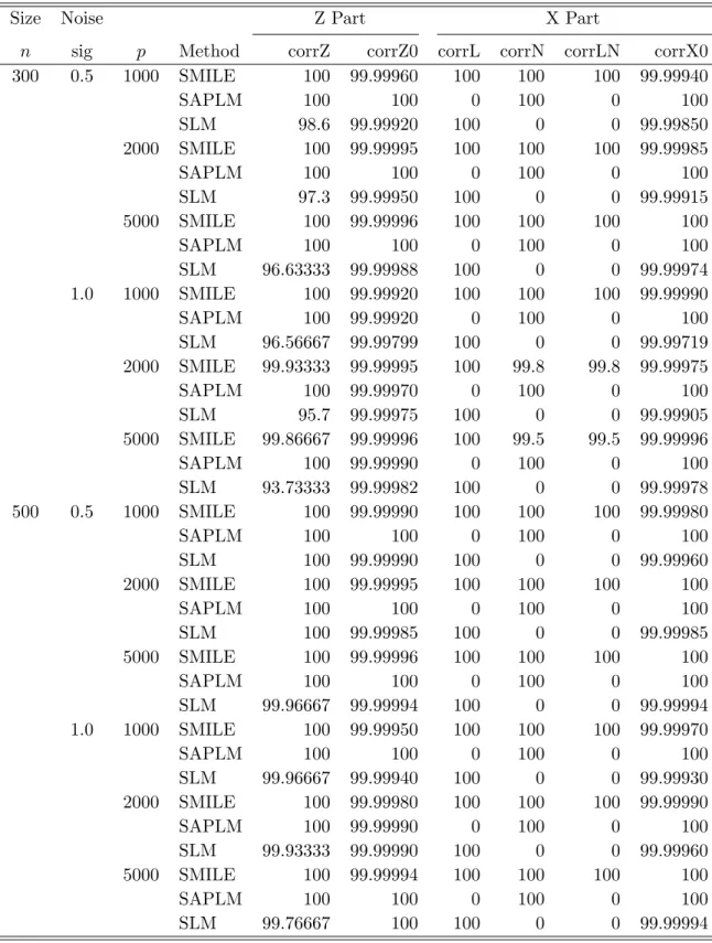
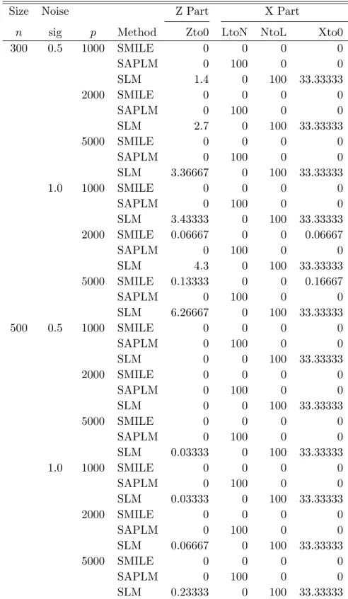
The model selection results are provided in Tables 1 and 2, respectively. SMILE can effectively identify informative linear and nonlinear components as well as correctly discover the linear and nonlinear structure in covariateX, while SAPLM neglects linear structure inX

and SLM fails in representing the nonlinear part of covariate X. For SMILE, the numbers of correctly selected nonzero covariates inZ, linear, nonlinear, linear-and-nonlinear components in

X, nonzero covariates are very close to ORACLE (100% for corrZ, corrL, corrN, corrLN, corrZ0 and corrX0, respectively); and the numbers of incorrectly identified components approach to 0 as the sample size n increases, as shown in Table 2. SMILE is close in the selection of covariatesZto the SAPLM estimator, and it far outperforms SAPLM in identifying the linear-and-nonlinear structure of covariate X. From the results in Tables 1 and 2, it is also evident that model misspecification leads to poor variable selection performance for SLM. Especially for the selection of covariates in X, which is our main focus for real data analysis, SLM fails to select the right nonlinear components in each simulation.

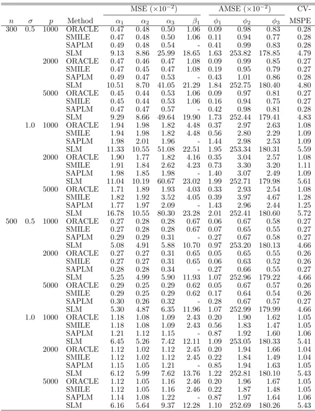
The estimation and prediction results are displayed in Table 3. Specifically, we present the MSEs for linear coefficients α1, α2, α3 and β1 and AMSEs for functions φ1, φ2 and φ3 and the CV-MSPEs for predicting Y. The case with known active covariates (ORACLE) is also reported in each setting and serves as a gold standard. SMILE performs the best in predicting

Y and estimating the coefficients of covariatesZ, as indicated by CV-MSPE and MSEs forα1, α2 andα3 that are closest to ORACLE in most simulation settings, while SLM is much higher (around 2 ∼ 18 times higher). As for the linear structure in X, as shown in MSE forβ1 and AMSE for φ1, the performance of SMILE is comparable to SAPLM and SLM, even though restricted to the selection bias; as the sample size n increases, the performance of SMILE is perfect and matches with ORACLE. Note that the SAPLM estimator is incapable in estimating

β1 in this case. The estimation of nonlinear functions φ2 and φ3 is also good for SMILE, and matches with ORACLE as sample size n increases. The inferior performance of SAPLM and the poor performance of SLM, in both estimation and prediction, illustrates the importance and necessity of identifying correct model structure.

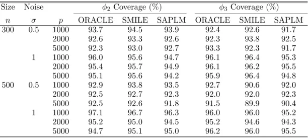
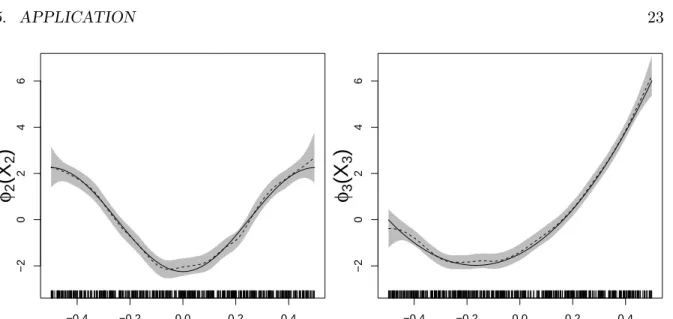
Next we investigate the coverage rates of the proposed SCB. For each replication, we test whether the true functions are covered by the SCB at the simulated values of the covariate in the interval [−0.5 +h,0.5−h], wherehis the bandwidth. Table 4 shows the empirical coverage probabilities for a nominal 95% confidence level out of 500 replications. For comparison, we also provide the SCBs from the SAPLM and ORACLE estimators. From Table 4, we observe that coverage probabilities for the SMILE, SAPLM and ORACLE SCBs all approach the nominal levels asnincreases, which provides positive confirmation of Theorem 4. In most cases, SMILE

Table 1: Statistics (B-i)–(B-vi) comparing the SMILE, SAPLM and SLM.

Size Noise Z Part X Part

n sig p Method corrZ corrZ0 corrL corrN corrLN corrX0

300 0.5 1000 SMILE 100 99.99960 100 100 100 99.99940 SAPLM 100 100 0 100 0 100 SLM 98.6 99.99920 100 0 0 99.99850 2000 SMILE 100 99.99995 100 100 100 99.99985 SAPLM 100 100 0 100 0 100 SLM 97.3 99.99950 100 0 0 99.99915 5000 SMILE 100 99.99996 100 100 100 100 SAPLM 100 100 0 100 0 100 SLM 96.63333 99.99988 100 0 0 99.99974 1.0 1000 SMILE 100 99.99920 100 100 100 99.99990 SAPLM 100 99.99920 0 100 0 100 SLM 96.56667 99.99799 100 0 0 99.99719 2000 SMILE 99.93333 99.99995 100 99.8 99.8 99.99975 SAPLM 100 99.99970 0 100 0 100 SLM 95.7 99.99975 100 0 0 99.99905 5000 SMILE 99.86667 99.99996 100 99.5 99.5 99.99996 SAPLM 100 99.99990 0 100 0 100 SLM 93.73333 99.99982 100 0 0 99.99978 500 0.5 1000 SMILE 100 99.99990 100 100 100 99.99980 SAPLM 100 100 0 100 0 100 SLM 100 99.99990 100 0 0 99.99960 2000 SMILE 100 99.99995 100 100 100 100 SAPLM 100 100 0 100 0 100 SLM 100 99.99985 100 0 0 99.99985 5000 SMILE 100 99.99996 100 100 100 100 SAPLM 100 100 0 100 0 100 SLM 99.96667 99.99994 100 0 0 99.99994 1.0 1000 SMILE 100 99.99950 100 100 100 99.99970 SAPLM 100 100 0 100 0 100 SLM 99.96667 99.99940 100 0 0 99.99930 2000 SMILE 100 99.99980 100 100 100 99.99990 SAPLM 100 99.99990 0 100 0 100 SLM 99.93333 99.99990 100 0 0 99.99960 5000 SMILE 100 99.99994 100 100 100 100 SAPLM 100 100 0 100 0 100 SLM 99.76667 100 100 0 0 99.99994

Table 2: Statistics (C-i)–(C-iv) comparing the SMILE, SAPLM and SLM.

Size Noise Z Part X Part

n sig p Method Zto0 LtoN NtoL Xto0

300 0.5 1000 SMILE 0 0 0 0 SAPLM 0 100 0 0 SLM 1.4 0 100 33.33333 2000 SMILE 0 0 0 0 SAPLM 0 100 0 0 SLM 2.7 0 100 33.33333 5000 SMILE 0 0 0 0 SAPLM 0 100 0 0 SLM 3.36667 0 100 33.33333 1.0 1000 SMILE 0 0 0 0 SAPLM 0 100 0 0 SLM 3.43333 0 100 33.33333 2000 SMILE 0.06667 0 0 0.06667 SAPLM 0 100 0 0 SLM 4.3 0 100 33.33333 5000 SMILE 0.13333 0 0 0.16667 SAPLM 0 100 0 0 SLM 6.26667 0 100 33.33333 500 0.5 1000 SMILE 0 0 0 0 SAPLM 0 100 0 0 SLM 0 0 100 33.33333 2000 SMILE 0 0 0 0 SAPLM 0 100 0 0 SLM 0 0 100 33.33333 5000 SMILE 0 0 0 0 SAPLM 0 100 0 0 SLM 0.03333 0 100 33.33333 1.0 1000 SMILE 0 0 0 0 SAPLM 0 100 0 0 SLM 0.03333 0 100 33.33333 2000 SMILE 0 0 0 0 SAPLM 0 100 0 0 SLM 0.06667 0 100 33.33333 5000 SMILE 0 0 0 0 SAPLM 0 100 0 0 SLM 0.23333 0 100 33.33333

Table 3: Estimation results comparing the ORACLE, SMILE, SAPLM and SLM. MSE (×10−2_{) AMSE (×10}−2₎ CV-n σ p Method α1 α2 α3 β1 φ1 φ2 φ3 MSPE 300 0.5 1000 ORACLE 0.47 0.48 0.50 1.06 0.09 0.98 0.83 0.28 SMILE 0.47 0.48 0.50 1.06 0.11 0.94 0.77 0.28 SAPLM 0.49 0.48 0.54 - 0.41 0.99 0.83 0.28 SLM 9.13 8.86 25.99 18.65 1.63 253.82 178.85 4.79 2000 ORACLE 0.47 0.46 0.47 1.08 0.09 0.99 0.85 0.27 SMILE 0.47 0.45 0.47 1.08 0.19 0.95 0.79 0.27 SAPLM 0.49 0.47 0.53 - 0.43 1.01 0.86 0.28 SLM 10.51 8.70 41.05 21.29 1.84 252.75 180.40 4.80 5000 ORACLE 0.45 0.44 0.53 1.06 0.09 0.97 0.81 0.27 SMILE 0.45 0.44 0.53 1.06 0.16 0.94 0.75 0.27 SAPLM 0.47 0.47 0.57 - 0.42 0.98 0.81 0.28 SLM 9.29 8.66 49.64 19.90 1.73 252.44 179.41 4.83 1.0 1000 ORACLE 1.94 1.98 1.82 4.48 0.37 2.97 2.63 1.08 SMILE 1.94 1.98 1.82 4.48 0.56 2.80 2.29 1.09 SAPLM 1.98 2.01 1.96 - 1.44 2.98 2.53 1.09 SLM 11.33 10.55 51.08 22.51 1.95 253.34 180.31 5.59 2000 ORACLE 1.90 1.77 1.82 4.16 0.35 3.04 2.57 1.08 SMILE 1.91 1.84 2.62 4.23 0.73 3.30 3.20 1.11 SAPLM 1.98 1.85 1.98 - 1.40 3.07 2.49 1.09 SLM 11.04 10.19 60.67 23.02 1.99 252.71 179.98 5.61 5000 ORACLE 1.71 1.89 1.93 4.03 0.33 2.93 2.54 1.08 SMILE 1.82 1.92 3.52 4.05 0.39 3.97 4.67 1.28 SAPLM 1.77 1.97 2.09 - 1.43 2.96 2.44 1.25 SLM 16.78 10.55 80.30 23.28 2.01 252.41 180.60 5.72 500 0.5 1000 ORACLE 0.27 0.28 0.28 0.67 0.06 0.67 0.58 0.27 SMILE 0.27 0.28 0.28 0.67 0.07 0.65 0.55 0.27 SAPLM 0.29 0.29 0.31 - 0.27 0.67 0.58 0.27 SLM 5.08 4.91 5.88 10.70 0.97 253.20 180.13 4.66 2000 ORACLE 0.27 0.27 0.31 0.65 0.05 0.65 0.55 0.26 SMILE 0.27 0.27 0.31 0.65 0.06 0.63 0.52 0.26 SAPLM 0.28 0.28 0.34 - 0.27 0.66 0.55 0.27 SLM 5.25 4.99 5.90 11.93 1.07 252.96 179.22 4.66 5000 ORACLE 0.29 0.25 0.29 0.62 0.05 0.67 0.57 0.26 SMILE 0.29 0.25 0.29 0.62 0.17 0.64 0.54 0.26 SAPLM 0.30 0.26 0.32 - 0.28 0.67 0.57 0.27 SLM 5.30 4.87 6.35 11.96 1.07 252.99 179.99 4.66 1.0 1000 ORACLE 1.18 1.08 1.09 2.43 0.20 1.90 1.62 1.05 SMILE 1.18 1.08 1.09 2.43 0.56 1.83 1.47 1.05 SAPLM 1.21 1.12 1.15 - 0.87 1.92 1.60 1.06 SLM 6.45 5.26 7.42 12.11 1.09 253.05 180.33 5.41 2000 ORACLE 1.12 1.02 1.12 2.45 0.20 1.94 1.66 1.04 SMILE 1.12 1.02 1.12 2.45 0.22 1.84 1.49 1.04 SAPLM 1.15 1.05 1.21 - 0.85 1.94 1.63 1.05 SLM 6.12 5.99 7.62 13.76 1.22 252.81 180.10 5.43 5000 ORACLE 1.12 1.05 1.16 2.46 0.20 1.96 1.67 1.05 SMILE 1.12 1.05 1.16 2.46 0.22 1.87 1.48 1.05 SAPLM 1.14 1.08 1.22 - 0.87 1.97 1.64 1.06 SLM 6.16 5.64 9.37 12.28 1.10 252.69 180.26 5.43

performs as well as or better than SAPLM, and arrives at about the nominal coverage when

n= 500 and σ = 1.0. Figure 1 depicts the true functionφ`, the corresponding SMILEφbSBLL<sub>`</sub> and the 95% SCB for φ` based on φbSBLL<sub>`</sub> , for `= 2,3, which are based on a typical run with

n= 500,p= 1000 andσ = 1.0.

Table 4: Coverage rates comparing the ORACLE, SMILE and SAPLM.

Size Noise φ2 Coverage (%) φ3 Coverage (%)

n σ p ORACLE SMILE SAPLM ORACLE SMILE SAPLM

300 0.5 1000 93.7 94.5 93.9 92.4 92.6 91.7 2000 92.6 93.3 92.6 92.3 93.8 92.5 5000 92.3 93.0 92.7 93.3 92.3 91.7 1 1000 96.0 95.6 94.7 96.1 96.4 95.3 2000 95.4 95.7 94.9 96.1 96.2 95.5 5000 95.1 95.6 94.2 95.9 96.4 94.8 500 0.5 1000 92.9 93.8 93.5 92.7 90.6 92.0 2000 92.5 92.7 92.3 92.0 92.0 92.3 5000 92.5 92.6 91.8 91.5 89.9 90.4 1 1000 97.1 96.7 96.3 96.0 96.0 95.2 2000 95.2 95.0 94.5 95.2 94.6 94.3 5000 94.7 95.1 95.0 96.2 96.0 95.5

Appendices B–D contain the results of additional simulations which show that our pro-posed SMILE procedure performs well relative to competing methods under a wider range of conditions.

5

Application

We illustrate the application of our proposed method in the ultra-high-dimensional setting by using the SAM data generated by Leiboff et al. (2015). The maize SAM is a small pool of stem cells located in the plant shoot that generate all the above-ground tissues of maize plants. Leiboff et al. (2015) showed that SAM volume is correlated with a variety of agronomically important traits in adult plants. The goal of our analysis is to model and predict SAM volume as a function of single nucleotide polymorphism (SNP) genotypes and messenger RNA transcript abundance levels using data from maize inbred lines. Following the preprocessing steps described in Section B.5 in the Supplementary Materials in Li et al. (2018), linear sure independent screening (Fan and Lv, 2008) for SNP genotypes, and nonlinear independent screening (Fan et al., 2011) for RNA transcripts, the dataset we analyze c onsists of log-scale SAM volume measurements, binary SNP genotypes at p1 = 5203 markers, and log-scale measures of abundance for p2 = 1020 transcripts for each ofn= 368 maize inbred lines.

−0.4 −0.2 0.0 0.2 0.4 −2 0 2 4 6

X

φ

(X

)

X

φ

(X

)

Figure 1: Plots of the SMILE (dashed curve) and the 95% SCB (shaded area) of the nonpara-metric component φ`(x`),`= 2,3 (solid curve).

Li et al. (2018) used the APLM to model the relationship between the log SAM volume response and predictors determined by SNP genotypes and RNA transcript abundance levels. Because the SNP genotypes are binary, they naturally entered the linear part of the APLM, and for convenience all the RNA transcripts were included in the nonlinear part of the APLM in Li et al. (2018). As discussed before, failing to account for exactly linear features makes the APLM less efficient statistically and computationally. In the following we apply our pro-posed SMILE method to distinguish among RNA transcripts entering the nonparametric and parametric parts of the APLM and to identify significant SNP genotypes and RNA transcripts simultaneously.

To compare the results of SMILE to the sparse APLM and the sparse linear regression model, we also analyze the data using the SAPLM and SLM estimators presented in Li et al. (2018). Parallel to the settings in Section 4, we use constant B-splines with four quantile knots for model structure identification, and use cubic B-splines with one quantile knot for nonlinear function approximation. We use the iterative algorithm proposed in Section 4.2 for penalty parameter selection and estimation.

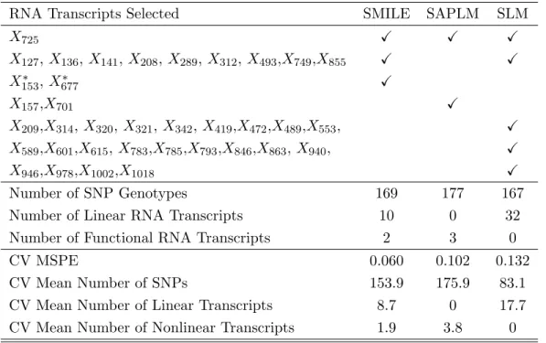
As shown in Table 5, SMILE identified 169 SNPs, 10 RNA transcripts linearly associated with log SAM size and 2 RNA transcripts that have nonlinear association with log SAM size. In contrast, SAPLM selected 177 SNPs and 3 RNA transcripts, and SLM selected 167 SNPs and 32 RNA transcripts. To evaluate the predictive performance of the two methods, we computed 10-fold cross-validation mean squared prediction error (CV-MSPE) for each method.

The SMILE-estimated nonlinear function for the selected nonlinear RNA transcript is plotted, along with 95% SCBs, in Figure 2.

Table 5: Selected SNPs and Transcripts by SMILE, SAPLM and SLM.

RNA Transcripts Selected SMILE SAPLM SLM

X725 X X X X127,X136,X141,X208,X289,X312,X493,X749,X855 X X X₁₅₃∗ ,X₆₇₇∗ X X157,X701 X X209,X314,X320,X321,X342,X419,X472,X489,X553, X X589,X601,X615,X783,X785,X793,X846,X863,X940, X X946,X978,X1002,X1018 X Number of SNP Genotypes 169 177 167

Number of Linear RNA Transcripts 10 0 32

Number of Functional RNA Transcripts 2 3 0

CV MSPE 0.060 0.102 0.132

CV Mean Number of SNPs 153.9 175.9 83.1

CV Mean Number of Linear Transcripts 8.7 0 17.7

CV Mean Number of Nonlinear Transcripts 1.9 3.8 0

∗nonlinear association identified by SMILE for X153 and X677

6

Discussion

This paper focuses on the simultaneous sparse model identification and learning for ultra-high-dimensional APLMs which strikes a delicate balance between the simplicity of the standard linear regression models and the flexibility of the additive regression models. We proposed a two-stage penalization method, called SMILE, which can efficiently select nonzero components and identify the linear-and-nonlinear structure in the functional terms, as well as simultane-ously estimate and make inference for both linear coefficients and nonlinear functions. First, we have devised a groupwise penalization method in the APLM for simultaneous variable selection and structure identification. After identifying important covariates and the functional forms for the selected covariates, we have further constructed SCBs for the nonzero nonparamet-ric functions based on refined spline-backfitted local-linear estimators. Our simulation studies and applications demonstrate the proposed SMILE procedure can be more efficient than

penal-−0.4 −0.2 0.0 0.2 0.4 −0.20 −0.10 0.00

X

φ

(

⋅

)

X

φ

(

⋅

)

Figure 2: Plot of the SMILE (solid curve) and the 95% confidence band (shaded area) for the selected RNA transcript.

ized linear regression and the penalized APLM without model identification, and can improve predictions.

Our work differs from previous works in practical, theoretical and computational aspects: (i) We perform variable selection and model structure identification simultaneously, for both the linear components in Z, and the linear and nonlinear forms for the components of X. In contrast, existing works either performs only model structure identification or performs variable selection only for components in X. (ii) Besides the consistency of model structure identification, we also provide inference tools for both the regression coefficients and the com-ponent functions. (iii) Compared to the local quadratic approximation approach used in Lian et al. (2015), which cannot provide exactly zero solutions and is inefficient for fitting large regression problems, our proposed iterative group coordinate descent algorithm takes advan-tage of sparsity in computation and is able to deal with the triple penalization problem very efficiently. (See Breheny and Huang (2015) for a detailed comparison of these two algorithms.) Our algorithm is easy to implement and can provide analysis results for large data sets with thousands of dimensions within seconds.

Our work deals with independent observations but can be extended to longitudinal data settings through marginal models or mixed-effects models. In addition, although we consider continuous response variables in our work, or approach can be readily extended to generalized additive partially linear models, to deal with different types of responses. Currently, the APLM assumes that the effects of all covariates are additive, which may overlook the potential interaction between covariates. Our method can be extended to models that can accommodate interactions between covariates, for example, APLMs with interaction terms. We leave such

extensions to future work. Another limitation of our work is a reliance on the assumption of constant error variance. However, heteroscedasticity may be encountered in the analysis of genomic data sets. It is of interest to develop a new methodology that allows non-constant error variance for high-dimensional estimation and model selection, and this is another challenge we leave for future work.

Acknowledgment

This work was supported by the Iowa State University Plant Sciences Institute Scholars Pro-gram. In addition, Wang’s research was supported by NSF grant DMS-1542332, and Nettle-ton’s research was supported by NSF grant IOS-1238142. We sincerely thank the Editor, the Associate Editor and the anonymous reviewers for their insightful comments that have lead to significant improvements on the paper.

Appendices

A. Effect of Smoothing Parameters on Performance of SMILE

To implement the proposed SMILE procedure, one needs to select the knots for a spline at the selection stage and refitting stage, and the bandwidth for a kernel at the backfitting stage. In this section, we study how these smoothing parameters affect the proposed SMILE method and evaluate the practical performance in the finite-sample simulation studies described in Section 4.2 of the main paper. In the literature of polynomial spline smoothing, the knots for a spline are generally put on a grid of equally spaced sample quantiles (Ruppert, 2002). Therefore, we only need to investigate the effect of the number of knots on the performance of SMILE.

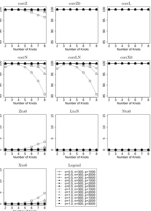
At the first stage (model selection), we use piecewise constant splines with the number of interior knots N = 2,3, . . . ,8 in the simulation. Figure A.1 shows the effect of N on the accuracy of model selection based on the criteria defined in the main paper: (B-i)–(B-vi) and (C-i)–(C-iv). From Figure A.1, it appears that the value N has little effect on the selection results. For all combinations ofn,pand σ, no matter whichN is used, the “corrZ0”, “corrL”, “corrX0” are all 100%, and the “LtoN” and “Nto0” are all 0%. The values of “corrZ”, “corrN”, “corrLN” and “Zto0” and “Xto0” are not exactly the same when using different values of N, but they are almost constant for N = 2,3, . . . ,8. Especially when the sample size n = 500, the proposed SMILE is able to identify the true model structure regardless of p= 1000,2000 or 5000. When n = 300 and p = 5000, the selection results become slightly worse when we

increase to N ≥6.

In summary, the values ofN often have little effect on the model selection results. Choosing small values ofN can also help to reduce computational burden. So we recommend using fewer knots at the model selection stage, especially when the sample size is small compared to the number of predictors. In practice, N = 2∼5 usually would be adequate to identify the model structure.

Next, we study the effect of the smoothing parameters at the refitting stage. For the selected model, we approximate the nonlinear functional components using higher order poly-nomial splines to obtain more accurate pilot estimators. Then we apply spline backfitted local-linear smoothing to obtain the final SBLL estimators and the corresponding SCBs. According to Assumption (A60), to obtain the SCB with the desired confidence level, the number of inte-rior knotsMnfor a refitting spline needs to satisfy: {n1/(2d)∨n4/(10d−5)} Mnn1/3, where

dis the degree of the polynomial spline basis functions used in the refitting. The widely used quadratic/ cubic splines and any polynomial splines of degree d≥2 all satisfy this condition. Therefore, in practice we suggest choosing

Mn= min{bn1/(2d)∨4/(10d−5)ln(n)c,bn/(4s)c}+ 1,

wheresis the number of nonlinear components selected at the first stage and the termbn/(4s)c

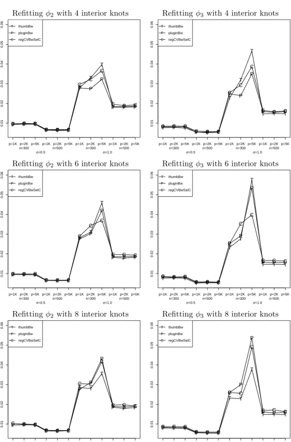
is to guarantee that we have at least four observations in each subinterval between two adjacent knots to avoid getting (near) singular design matrices in the spline smoothing. A researcher with some knowledge of the shape of the nonlinear component may be able to select a more suitable number of knots. In our simulation studies, we try 4, 6 and 8 interior knots to test the sensitivity of the SBLL estimators and the corresponding SCBs.

For the local-linear smoothing in the backfitting, Condition (B2) requires that the band-widths are of ordern−1/5. Any bandwidths with this rate lead to the same limiting distribution forφbSBLL_` , so the user can consider any standard routine for bandwidth selection. There have been many proposals for bandwidth selection in the literature. In our simulation, we consider three popular bandwidth selectors described in Fan and Gijbels (1996) and Wand and Jones (1995): rule-of-thumb bandwidth (“thumbBw”), plug-in bandwidth selector (“pluginBw”) and leave-one-out cross-validation bandwidth selector (“regCVBwSelC”). Below we present simu-lation results to compare the performance of three bandwidth selectors. The kernel that we use here is the Epanechnikov kernel: K(u) = 3/4(1−u2)I(|u| ≤1).

To see how the refitting smoothing parameters affect estimation accuracy, we report the average mean square errors (AMSEs) of the SBLL estimators based on 4, 6 and 8 interior knots in the spline refitting and three different bandwidth selectors in the kernel backfitting. Figure A.2 presents the AMSEs of the resulting SBLL estimators based on different combinations of

corrZ corrZ0 corrL 2 3 4 5 6 7 8 85 90 95 100 Number of Knots 2 3 4 5 6 7 8 85 90 95 100 Number of Knots 2 3 4 5 6 7 8 85 90 95 100 Number of Knots

corrN corrLN corrX0

2 3 4 5 6 7 8 85 90 95 100 Number of Knots 2 3 4 5 6 7 8 85 90 95 100 Number of Knots 2 3 4 5 6 7 8 85 90 95 100 Number of Knots

Zto0 LtoN Nto0

2 3 4 5 6 7 8 0 5 10 15 Number of Knots 2 3 4 5 6 7 8 0 5 10 15 Number of Knots 2 3 4 5 6 7 8 0 5 10 15 Number of Knots Xto0 Legend 2 3 4 5 6 7 8 0 5 10 15 Number of Knots

the refitting smoothing parameters. For both φ1 and φ2, the AMSEs are very similar across the different combinations of knots and bandwidth selectors.

Figure A.3 shows the coverage rates of the SCBs based on different combinations of knots and bandwidth selectors. From Figure A.3, it is clear that the number of knots for a spline in the refitting has very little effect on the coverage of the SCBs. One also observes that the performances of the SCBs based on different smoothing parameters become more similar with increasing sample size, whereas the coverage rates of the SCBs using the “thumbBw” selector are the closest to the nominal level in all the simulation settings. Thus we recommend the “thumbBw” selector, especially when the sample size is small.

B. Simulation Studies Using Purely Additive Models or Purely

Linear Models

In this section, we examine the performance the proposed method when the underlying model is either a purely additive model (AM) or a purely linear model (LM). We evaluated the selection, estimation and prediction accuracy, and inference performance of the proposed SMILE method. We also compared the performance of SMILE with the sparse APLM estimator with adaptive group LASSO penalty (SAPLM), the ordinary linear least squares estimator with the adaptive LASSO penalty (SLM), and the oracle estimator (ORACLE), which uses the same estimation techniques as the SMILE except that no penalization or data-driven variable selection is used because all active and inactive index sets are treated as known. All the performance measures were computed based on 200 replicates.

Case I. A Purely Additive Model. We generate simulated datasets using the AM structure

Yi = p X `=1 φ`(Xi`) +εi, where φ1(x) = 8 sin(2πx) 2−sin(2πx) −E 8 sin(2πX1) 2−sin(2πX1) ,

φ2(x) =−3 cos2(πx) + 6 sin2(πx)−E{−3 cos2(πX2+ 6 sin2(πX2)}, φ3(x) = 6x+ 18x2−E(6X3+ 18X32),

and φ4(x) =. . .=φp(x) = 0.

Case II. A Purely Linear Model. We generate simulated datasets using the LM structure:

Yi=

p

X

`=1