Statistical Methods for Large Spatial and Spatio-temporal Datasets

(1)

STATISTICAL METHODS FOR LARGE SPATIAL AND SPATIO-TEMPORAL DATASETS

A Dissertation by

BOHAI ZHANG

Submitted to the Office of Graduate and Professional Studies of Texas A&M University

in partial fulfillment of the requirements for the degree of DOCTOR OF PHILOSOPHY

Chair of Committee, Jianhua Huang Co-Chair of Committee, Huiyan Sang Committee Members, Mikyoung Jun

Renyi Zhang Head of Department, Valen Johnson

August 2015

Major Subject: Statistics

(2)

ABSTRACT

Classical statistical models encounter the computational bottleneck for large spatial/spatio-temporal datasets. This dissertation contains three articles describ-ing computationally efficient approximation methods for applydescrib-ing Gaussian process models to large spatial and spatio-temporal datasets.

The first article extends the FSA-Block approach in [60] in the sense of preserv-ing more information of the residual covariance matrix. By uspreserv-ing a block conditional likelihood approximation to the residual likelihood, the residual covariance of neigh-boring data blocks can be preserved, which relaxes the conditional independence assumption of the FSA-Block approach. We show that the approximated likelihood by the proposed method is Gaussian with an explicit form of covariance matrix, and the computational complexity is linear with sample size n. We also show that the proposed method can result in a valid Gaussian process so that both the parame-ter estimation and prediction are consistent in the same model framework. Since neighborhood information are incorporated in approximating the residual covariance function, simulation studies show that the proposed method can further alleviate the mismatch problems in predicting responses on block boundary locations.

The second article is the spatio-temporal extension of the FSA-Block approach, where we model the space-time responses as realizations from a Gaussian process model of spatio-temporal covariance functions. Since the knot number and locations are crucial to the model performance, a reversible jump Markov chain Monte Carlo (RJMCMC) algorithm is proposed to select knots automatically from a discrete set of spatio-temporal points for the proposed method. We show that the proposed knot selection algorithm can result in more robust prediction results. Then the proposed

(3)

method is compared with weighted composite likelihood method through simulation studies and an ozone dataset.

The third article applies the nonseparable auto-covariance function to model the computer code outputs. It proposes a multi-output Gaussian process emulator with a nonseparable auto-covariance function to avoid limitations of using separable em-ulators. To facilitate the computation of nonseparable emulator, we introduce the FSA-Block approach to approximate the proposed model. Then we compare the proposed method with Gaussian process emulator with separable covariance models through simulated examples and a real computer code.

(4)

ACKNOWLEDGEMENTS

I would like to gratefully and sincerely thank my advisors Dr. Jianhua Huang and Dr. Huiyan Sang, for their guidance, supports, and encouragements during my Ph.D. study. Your passion, inspiration, generosity, and patience make me have a wonderful journey in statistics, and also let me determine to pursue the academic career. Without your help, I would never accomplish so much. It is my honor to work with both of you and I will cherish this experience.

I would also like to thank my committee members Dr. Mikyoung Jun and Dr. Renyi Zhang, for your helpful comments in my preliminary exam. Your valuable suggestions help me improve my dissertation and make it more complete.

I would like to thank the Department of Statistics at Texas A&M University, for its wonderful Ph.D. program, excellent faculty members, and powerful computing resources. I would also like to thank the SGSA, for organizing department events and hosting company recruitments.

Finally, I would like to thank my parents, for their understandings and supports during my graduate study. Also a big thank you to my deer friends; without your company and kind help, it would be much harder to complete a Ph.D. degree.

(5)

TABLE OF CONTENTS

Page

ABSTRACT . . . ii

ACKNOWLEDGEMENTS . . . iv

TABLE OF CONTENTS . . . v

LIST OF FIGURES . . . viii

LIST OF TABLES . . . x

1. INTRODUCTION . . . 1

1.1 Gaussian Process Model . . . 1

1.2 Popular Approximation Methods for Gaussian Process Model . . . . 3

1.2.1 Low-rank approximation models . . . 3

1.2.2 Sparse approximation methods . . . 4

1.2.3 Composite likelihood approach . . . 5

1.3 Overall Structure . . . 6

2. A SMOOTH FULL-SCALE APPROXIMATION APPROACH FOR LARGE SPATIAL DATASETS . . . 8

2.1 Introduction . . . 8

2.2 Methodology . . . 11

2.2.1 The spatial regression model . . . 11

2.2.2 The FSA-Block approach . . . 12

2.2.3 The proposed approach . . . 14

2.2.4 Relations to previous methods . . . 16

2.2.5 Computational complexity of the SFSA approach . . . 18

2.2.6 Choices of tuning parameters . . . 19

2.3 Parameter Estimation and Prediction . . . 20

2.3.1 Maximum likelihood estimators . . . 20

2.3.2 Bayesian inference on model parameters . . . 21

2.3.3 Prediction . . . 22

2.3.4 The Smooth FSA spatial process . . . 24

2.4 Simulation Study . . . 26

(6)

2.4.2 Prediction on block boundaries . . . 31

2.5 Real Data Analysis . . . 34

2.6 Discussion . . . 36

3. FULL-SCALE APPROXIMATIONS OF SPATIO-TEMPORAL COVARI-ANCE MODELS . . . 38

3.2 The FSA Approach . . . 41

3.2.1 Model . . . 41

3.2.2 Covariance approximation of spatio-temporal process . . . 42

3.2.3 Fast computation of parameter estimation and spatio-temporal prediction . . . 46

3.2.4 Selection of tuning parameters . . . 48

3.2.5 Further improvement of computational efficiency by pre-tapering 51 3.3 Simulation Studies . . . 52

3.3.1 Simulation study 1 . . . 52

3.3.2 Simulation study 2 . . . 58

3.4 Analysis of The Eastern US Ozone Data . . . 60

4. APPLICATIONS OF GAUSSIAN PROCESS MODEL TO UNCERTAIN-TY QUANTIFICATION OF COMPUTER CODE OUTPUTS . . . 67

4.2 Methodology . . . 70

4.2.1 Multivariate Gaussian process regression model . . . 71

4.2.2 Nonseparable auto-correlation models . . . 73

4.2.3 FSA-Block approximation . . . 75

4.3 Bayesian Inference of Model Parameters and Prediction . . . 79

4.3.1 Prior specifications . . . 79

4.3.2 Bayesian inference on the model parameters . . . 79

4.3.3 Prediction . . . 82

4.4 Numerical Results . . . 83

4.4.1 2-input and 1-output example . . . 83

4.4.2 Krainchnan-Orszag three-mode problem . . . 85

4.4.3 Flow through porous media example . . . 90

4.5 The Regenerator of A Carbon Capture Unit . . . 95

5. CONCLUSIONS . . . 102

(7)

APPENDIX A. PROOF OF THEOREMS . . . 114 A.1 Proof of Theorem 2.2.1 . . . 114 A.2 Proof of Theorem 2.3.1 . . . 116 APPENDIX B. CALCULATING THE APPROXIMATED π(θ|Y) BY THE

(8)

LIST OF FIGURES

FIGURE Page

2.1 Plots of residual covariance for 3 methods. . . 18 2.2 MSE of each covariance parameter against the number of neighboring

blocks for the SFSA approach. The simulation setting is the same as that described in Section 2.4.1; the covariance model is exponential model with φ= 1, σ2 _{= 1, and} _τ2 _{= 0}_._{01. . . .} ₃₀

2.3 MSPEs against the number of neighboring blocks for the SFSA ap-proach with K = 25,100. The simulation setting is the same as that described in Section 2.4.1; the covariance model is exponential model with φ= 1, σ2 = 1, and τ2 = 0.01. . . 31 3.1 513 ozone monitoring station locations and the estimated averaged

seasonal effect in 1999. . . 61 4.1 Predictive surface of input space of y1 at time points 5 and 10 using

the nonseparable model. . . 87 4.2 Predictive surface of input space of y2 at time points 5 and 10 using

the nonseparable model. . . 88 4.3 Predictive surface of input space of y3 at time points 5 and 10 using

the nonseparable model. . . 88 4.4 The MSPEs averaged over time by the nonseparable model. . . 89 4.5 The predictive mean curve in time by the nonseparable model. The

blue line is the predictive mean curve of time; the dash lines are corre-sponding 95% confidence intervals; the red dots are the means of the computer code outputs. . . 90 4.6 Predictive mean surfaces by the nonseparable model versus the Monte

Carlo estimates based on 24 input points. Upper panels: velocity in

y-direction uy; middle panels: velocity inx-direction ux; lower panels:

pressurep. . . 94 4.7 Predictive standard deviations by the nonseparable model. . . 95

(9)

4.8 Images of the solid volume fractions at time 271 for 2 input points. . 97 4.9 The left panels are predictive distributions of solid volume fractions

under different combinations of dp and K =vg/umf; the right panels

are corresponding computer code results. . . 99 4.10 Predictive mean input surfaces of 5 probabilities by the nonseparable

(10)

LIST OF TABLES

TABLE Page

2.1 Means and Mean Squared Errors (in parenthesis) of parameters in Mat´ern covariance model. The number of blocks K = 100 for all three methods and the results are based on 200 simulated datasets. . 28 2.2 MSPEs and MSEs of the exponential model with sample size 4000.

The number of blocks K = 100. . . 29 2.3 MSPEs and MSEs (in parenthesis) of the exponential model with

sam-ple size 4000. 360 boundary locations were held out for prediction. The number of blocks K = 100. . . 33 2.4 MSPEs of the exponential model with σ2 = 1 and a larger nugget

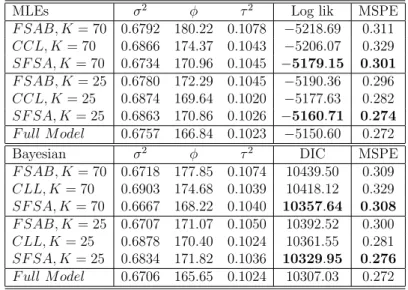
τ2 = 0.2. 360 boundary locations were held out for prediction. The number of blocks K = 100. . . 34 2.5 Maximum Likelihood and Bayesian inference results using the

expo-nential model. . . 35 3.1 The means and MSEs (in parenthesis) of each parameter and MSPE

results for covariance model with a nugget. The results are based on 100 runs of simulations. . . 54 3.2 The means and MSEs (in parenthesis) of each parameter and MSPE

results for the covariance model without nugget. The results are based on 100 runs of simulations. . . 56 3.3 The means and MSEs (in parenthesis) of each parameter and MSPE

results for Mat´ern’s covariance model. The results are based on 100 runs of simulations. . . 57 3.4 Parameter estimation and prediction results for FSA-Block approach

with knots selected by RJMCMC algorithm. For number of knots m, we report its posterior means. . . 60 3.5 Parameter estimation and prediction results of monthly data. The

root mean squared predictive errors (RMSPE) were made based on the within 4 days’ training data. . . 63

(11)

3.6 Parameter estimation and prediction results of summer ozone. Model A is the separable covariance model in (3.13) with space-time interac-tion parameter η= 0. Model B is the nonseparable covariance model in (3.13). And model C is the Mat´ern covariance model in (3.14). . . 65 3.7 Parameter estimation and prediction results of summer ozone datasets

by FSA-Block with random knot selection. . . 66 4.1 Posterior means and MSPEs. . . 84 4.2 Posterior means of model parameters and MSPEs. . . 86 4.3 Posterior means of model parameters and prediction results of each

output component. . . 93 4.4 Posterior means of model parameters and the overall MSPEs. . . 98

(12)

1. INTRODUCTION

1.1 Gaussian Process Model

Spatial and spatio-temporal datasets are widely observed in many disciplines, such as the climatology, geology and so on, where the datasets are labeled by spatial coordinates such as longitude and latitude, as well as time (for space-time data). An important characteristic of spatial/spatio-temporal data is that nearby observations (in space or space-time) tend to be more alike than those far apart [15]. For exam-ple, one simple way to forecast tomorrow’s weather is to use today or last few days’ weather; similar conclusion holds for the spatial data, such as studies in environments (i.e., ground pollutants, distribution of species). To characterize the dependence of the responses, the covariance functions are widely used. The interests lie in infer-ences of the spatial/spatio-temporal dependence structures and subsequently making predictions on unobserved locations.

The responses are usually treated as realizations of an underlying spatial/spatio-temporal process, and the most popular process model is the Gaussian process model. Let X = {x1,x2, . . . ,xn} be a set of locations, where xi = si for spatial data and xi = (si, ti) for space-time data. Let Y = (y(x1), y(x2), . . . , y(xn))T be a column

vector collecting the responses atX, then we assume that_Y∼ N(Zβ,C(θ)), where

Z is the n×p design matrix, β is ap×1 regression coefficients vector, and C(θ) is the covariance matrix depending on parameter vector θ. C(θ) is usually assumed to be generated from a positive-definite covariance function, such as Mat´ern covariance model [51]: C(x,x0;θ) = σ 2 Γ(ν)2 1−ν (h/φ)νKν(h/φ),

(13)

whereh=kx−x0k; Γ(·) is the gamma function,Kν(·) is the modified Bessel function

of the second kind, σ2 _{is the variance parameter,} _{φ >} _{0 is the dependence range}

parameter, and ν > 0 is the smoothness parameter. The log-likelihood function up to a constant is `(_Y|β,θ) =−1 2|C(θ)| − 1 2(Y−Zβ) T_C−1 (θ)(_Y−Zβ).

Given a predictive location xp and assume all parameters are known, then we have

the Best Linear Unbiased Predictor (BLUP),

ˆ

y(xp) =zT(xp)β+CpnC−1(θ)(Y−Zβ)

and the corresponding Mean Squared Error (MSE)

MSE(ˆy(xp)) = Cp− CpnC−1(θ)CpnT ,

wherez(xp) is thep×1 vector of covariates atxp,Cp =C(0;θ) andCpn=C(xp,X;θ).

From the log-likelihood function and the BLUP formula,C−1_{(θ) and}_|C_(θ)| _need

to be computed for model inference and prediction. To compute the inverse and de-terminant of the covariance matrix, we need to obtain the Cholesky factorL(θ) such that C(θ) = L(θ)LT(θ), which typically requires O(n3) Floating-points Operations Per Second (flops). Since the computation costs grow quickly with the sample size, the direct application of Gaussian process models to large spatial/spatio-temporal models can be computationally prohibitive for large datasets. This computational challenge motives the innovations of new statistical methods scalable to handle large datasets [67].

(14)

1.2 Popular Approximation Methods for Gaussian Process Model

In this Section, we will give brief summaries of Gaussian process approximation methods most related to this dissertation. The introduction part in each chapter will give more comprehensive literature reviews of related methods.

1.2.1 Low-rank approximation models

The basic idea of low-rank models is to project the original process y(x) to a low-dimensional space spanned by a small number of basis functions. Then the low-rank approximation methods seek to replace the original covariance matrix with an approximated rank matrix for computational efficiency. The popular low-rank models include the Predictive Process model [4, 21] and the Fixed Rank K-riging (FRK) model [13, 40]. Given a set of locations X∗ = {x∗₁, . . . , x∗_m}, re-ferred to as knots, the predictive process model approximates a zero-mean Gaussian process y(x) using the conditional mean process E(y(x)|y(X∗)), where y(X∗) = (y(x∗₁), y(x∗₂), . . . , y(x∗_m))T_{. The approximated covariance matrix by the predictive}

process model is

Cpp =Cn∗C∗−1Cn∗T ,

where Cn∗ = C(X,X∗;θ) and C∗ = C(X∗,X∗;θ). Cpp is positive semi-definite

with rankm. When the responses are observed with white noises, fast computations can be achieved by Sherman-Woodbury-Morrison inversion formula [35] with com-putational complexity O(nm2). Thus a small number of knots lead to significant reduction of computations.

Similarly to predictive process model, the FRK model assumes y(x) = ST₍_x_)η

(15)

ar×1 random vector following a Gaussian distributionN(0, K), whereK is ar×r

positive definite matrix to be estimated. The computational complexity of the FRK model is O(nr2_{), so it has good computational scalability. Also by construction of}

the covariance matrix, the FRK model can handle large datasets with nonstationary dependence structures.

Although the low-rank approximations has computational complexity linear with sample size n, it has several limitations. For example, when the dependence range of the data is small, the low-rank model usually needs a large number of basis func-tions for providing a satisfactory approximation to the original process. [63] gives a comprehensive discussion of limitations of low-rank models and points out that the best low-rank model can perform poorly when the data are strongly correlated for neighboring observations.

1.2.2 Sparse approximation methods

The sparse approximation methods replace the correlations of distance locations by zeros and only keep the correlations among neighboring locations. Covariance tapering [23, 43] is a popular method to induce sparsity for the covariance matrix. Given a covariance function C(·,·;θ), the tapered covariance is

Ctaper(x,x0) = C(x,x0;θ)K(kx−x0k;γ),

where K(x,x0;γ) is the tapering function which is positive definite and has zero val-ues when kx−x0k ≥ γ. Thus a small γ leads to a sparse covariance matrix when evaluating Ctaper(x,x0) on observed set X. The matrix decomposition algorithms

for sparse matrices are applied subsequently to compute the Cholesky factor of the approximated covariance matrix by the tapered covariance function. The computa-tional complexity is O(nr2_{), where} _r _{is the number of nonzero entries per row and}

(16)

column of a sparse matrix. By construction, the covariance tapering approach ig-nores the dependence of responses far apart, thus its performance is poor when the dependence range is large.

1.2.3 Composite likelihood approach

The composite likelihood approach approximates the full data likelihood function by a product of low-dimensional marginal or conditional likelihoods [49, 70]. Since evaluations of low-dimensional likelihoods are computationally cheaper, the compos-ite likelihood approach gains the computational efficiency. One simple composition likelihood approach is the independent blocks approximation [8, 63]. Given a par-tition of observed responses _Y = ∪K

k=1Yk, the independence blocks approximation

approximates the full likelihoodL(_Y;θ) by

K

Q

k=1

L(Yk;θ). If we choose relatively equal block size nb for each data block, the computational complexity of the independent

blocks approximation is O(nn2

b), so fast computations can be achieved if we choose

nb to be small.

Alternatively, [72, 64] approximates L(_Y;θ) by a product of conditional like-lihoods of data blocks, referred to as the block conditional likelihood approxima-tion. Motivated by the chain rule L(_Y;θ) =

K

Q

k=1

L(Yk|Y(k),θ), where Y(k) =

{Y1, . . . ,Yk−1} for k ≥ 1 and Y(1) = ∅, the block conditional likelihood

approx-imation approximates L(_Y;θ) by

K

Y

k=1

L(Yk|YN(k),θ),

where YN(k) ⊆ Y(k) contains all the neighboring data blocks for kth data block.

Computations of evaluating this approximated likelihood can be greatly reduced if

(17)

conditional likelihood approximation approach in [72, 64] for K = n can lead to a valid Gaussian likelihood. In addition, they show that a valid Gaussian process can be obtained by this approximation so that both parameter estimation and prediction of the proposed model can be performed in a unified framework.

1.3 Overall Structure

The following is the general structure of this dissertation. Section 2 extends the Full-Scale Approximation with Block modulating function [60], referred to as the FSA-Block approach, in the sense of preserving more information of the residual co-variance function. Given a partition_Y=∪K

k=1Yk, the FSA-Block approach assumes

thatYk’s are conditionally independent given the predictive process component. The

conditional independence assumption may be strong when the predictive process part does not perform well (e.g, the number of knots is small or the dependence structure is local). By using the block conditional likelihood approximation to the full residu-al likelihood, we show that the residuresidu-al covariance among neighboring Yk’s can be

preserved. Since more information are kept for the residual covariance, the proposed method enjoys better statistical efficiency. We also show that the proposed method can result in a valid Gaussian process model so that the parameter estimation and prediction are consistent. We compare the proposed method with the FSA-Block ap-proach and the block version of the nearest neighbor process apap-proach [18] through simulation studies and a real precipitation dataset.

Section 3 is a spatio-temporal extension of the FSA-Block approach, where we consider modeling the space-time responses by a Gaussian process with a spatial-temporal covariance function. In addition, we discuss selection methods of the knot set for the proposed method and introduce a Reversible Jump Markov chain Monte Carlo algorithm [33] to dynamically update the knot number and knot locations. We

(18)

demonstrate the effectiveness of proposed method using a simulated nonstationary dataset and an ozone data of eastern US.

Section 4 applies the FSA-Block approach to approximating the Gaussian pro-cess emulator for large computer code outputs. A multi-output Gaussian propro-cess emulator with a nonseparable auto-covariance function is proposed to avoid limita-tions of using separable emulators. To facilitate the computation of nonseparable emulator, the FSA-Block approach is applied to approximating the nonseparable auto-covariance function. We compare the performance of the proposed method with Gaussian process with separable auto-covariance function through simulated examples and a real computer code of the carbon capture system.

Summary and discussion of potential extensions are given in Section 5. The proofs of theorems in Section 2 and the algorithm of calculating the posterior distributions in Section 4 are provided in the Appendix.

(19)

2. A SMOOTH FULL-SCALE APPROXIMATION APPROACH FOR LARGE SPATIAL DATASETS

2.1 Introduction

Spatial datasets arising from ecology, climatology, and other disciplines have gen-erated considerable interests for scientists. With the advent of remote sensing and GPS techniques, the spatial data collection capacity increases dramatically and s-tatisticians nowadays are facing a large number of observations on variables of in-terest. The growth in data size imposes computational challenges to the classical statistical modeling methods [62, 5] and has driven the innovations of new methods scalable to handle large datasets [67].

One of the most popular models for spatial datasets is the Gaussian process mod-el, assuming finite observations are jointly Gaussian. Although the Gaussian process model enjoys the mathematical tractability and can provide prediction intervals for observations on unobserved locations, its computational complexity generally grows cubically with the sample size n, due to the expensive matrix factorizations. Specif-ically, the calculations of inverse and determinant of the data covariance involve the Cholesky decomposition of the finite sample covariance matrix, whose computation requires O(n3_{) floating point operations (flops). The evaluation of the Gaussian}

process model will be computationally prohibitive for very large n.

When the covariance matrix has a certain structure, such as the Toeplitz ma-trix [79], fast computations are available for evaluating the Gaussian process model. However, since the spatial process is generally observed at irregularly spaced loca-tions and the dependence of distant pairs of observaloca-tions is often nonnegligible, the data covariance matrix does not have any structures in general. Approaches tackling

(20)

the computational challenge have adopted two major paths. The first path is to approximate the full likelihood function by some simplified versions. The composite likelihood approach [49, 70], as a general class of pseudo-likelihoods, has been used to model spatial datasets. The idea is to approximate the ordinary likelihood using products of marginal or conditional likelihoods of reduced dimensions. For marginal composite likelihood approach, [16] proposed a composite likelihood approach based on marginal densities of pairwise differences of responses; also based on bivariate marginal densities, [69] proposed a pairwise composite likelihood approach for spa-tial generalized linear mixed models. Recently, [19] proposed to use a composite likelihood function defined as the product of joint densities of pairwise spatial blocks and it enjoys better statistical efficiency than the composite likelihood based on bi-variate marginal densities. For conditional composite likelihood approach, [72] and [64] constructed composite estimating functions based on conditional densities of spatial data blocks.

The second path is to approximate the data covariance matrix with either a low-rank or a sparse matrix whose matrix factorizations are computationally cheaper. The popular low-rank models include the Gaussian predictive process model [4] and the Fixed Rank Kriging model [13, 42], where the original spatial process is ap-proximated by a smoother process based on a small number of basis functions. For sparse matrix approximations, the covariance tapering method [23, 43] approximates the original covariance with a sparse matrix by shrinking the dependence of distant pairs of spatial locations to be zero. Then the algorithms for manipulating sparse matrices are applied to reduce the computational burden. Instead of working on the covariance matrix, the Gaussian Markov Random Field model [56, 48] induces a sparse precision matrix for facilitating computations.

(21)

and the covariance tapering method, on the contrary, can not capture the large-scale dependence well, [59] proposed a so-called Full-Scale Approximation approach (F-SA), which adds a sparse residual covariance component to the covariance of the Gaussian predictive process model, for approximating the data covariance well un-der both large and small scale dependence scenarios. Specifically, let C(·,·;θ) and Cl(·,·;θ) be the covariance functions of the original Gaussian process and Gaussian

predictive process, respectively, then the covariance function of the FSA approach is C† =Cl(·,·;θ) + (C(·,·;θ)− Cl(·,·;θ))K(·,·), where the function K, referred to as

the modulating function, is positive semi-definite and has a large number of zeros evaluated on observed spatial locations. If we choose K such that the residual co-variance is block-diagonal, then the method is called the FSA-Block approach; if some compactly supported covariance functions are chosen for K, then the method is called the FSA-Taper approach. [60] has shown that the FSA-Block approach can have better numerical results than the FSA-Taper approach.

This Section extends the FSA-Block approach in the sense of preserving more information of the residual covariance. By using a conditional likelihood approxima-tion, the dependence across blocks of the residual covariance is preserved by the new proposed approach. Since more information are kept for the data covariance matrix, we expect that the new proposed approach can perform better than the FSA-Block approach when the residual dependence across blocks is not negligible. In addition, the proposed method can produce a smoother prediction surface than that by the FSA-Block method by using the conditional likelihood approximation, so the mis-matches of predictions on boundary locations can be alleviated for the proposed method. We name the new proposed method the Smooth Full-Scale Approximation approach (SFSA). The approximated data covariance of the SFSA approach can re-duce to covariance of the FSA-Block approach and the covariance of the conditional

(22)

likelihood approximation approach proposed in [18]. Moreover, we show that the SFSA approach can define a valid Gaussian process, thus both the parameter es-timation and prediction can be performed under the unified framework. Since the covariance function is available for the SFSA approach, the kriging formula can be directly applied for predictions.

2.2 Methodology

2.2.1 The spatial regression model

LetY(s) be a response variable observed at a locations, where s belongs to the spatial domain S ⊆ _R2_{. We model} _Y₍_s_{) through the following spatial regression}

model

Y(s) = xT(s)β+w(s) +(s), (2.1)

wherex(s) is ap×1 vector of covariates,βis the corresponding regression coefficients vector, w(s) is a latent zero-mean Gaussian process, and (s) is a Gaussian white noise process with constant variance τ2_{, independent of} _w₍_s_{) . The covariance of}

the spatial process w(s) characterizes the spatial dependence structure and it is specified by a valid covariance function C(s,s0;θ) = Cov(w(s), w(s0)). For example, the Mat´ern covariance is widely used in spatial statistics due to its flexibility of modeling the smoothness of the spatial process,

C(s,s0;θ) = σ

2

Γ(ν)2

1−ν

(h/φ)νKν(h/φ), (2.2)

where Γ is the gamma function, Kν is the modified Bessel function of the second

kind,σ2 is the variance parameter, φ is the spatial dependence range parameter and

(23)

“nugget” effect, accounting for the measurement error effect.

Suppose Y(s) is observed at n spatial locations S = {s1, . . . ,sn}. Let Y =

(Y(s1), . . . , Y(sn))T denote then×1 observed response vector andX= (x(s1), . . . , x(sn))T

denote the n×p design matrix. Then the log-likelihood function is

`(_Y|θ,β) =−1 2|CY| − 1 2(Y−Xβ) T_C−1 Y (Y−Xβ) + constant, (2.3)

where the data covarianceC_Y=Cw+τ2InandCw = [C(si,sj)]i,j=1,...,nis the covariance

matrix of w(s) on S. Evaluating (2.3) requires O(n3_{) flops for calculating} _|C

Y| and

C−1

Y in general, so the computational cost can be very intensive or even prohibitive

when n is large.

2.2.2 The FSA-Block approach

Givenm locations S∗ ={s∗₁, . . . ,s∗_m}, referred to as knots, the predictive process model [4] approximates w(s) by the conditional mean process wl(s) = E(w(s)|w∗),

where w∗ = w(S∗) = (w(s∗₁), . . . , w(s∗_m))T. Since w(s) has zero mean, then wl(s) =

C(s,S∗_)C−1

∗ w∗, where C(s,S∗) = [C(s,si∗)]i=1,...,m and C∗ = [C(s∗i,s ∗

j)]i,j=1,...,m. The

spatial process w(s) can be decomposed into two independent processes

w(s) = wl(s) +ws(s),

where ws(s) is the exact residual process of w(s). Since the covariance function of

wl(s) isCl(s,s0) = C(s, S∗)C∗−1CT(s0, S∗), the covariance function ofws(s) isCs(s,s0) =

C(s,s0)− Cl(s,s0). By Schur complement property of linear algebra, Cs is positive

definite when S ∩S∗ = ∅ and positive semi-definite otherwise. Therefore, if we approximate w(s) only using wl(s), the covariance information in ws(s) will be lost.

(24)

variations of the process are not negligible [21, 63]. Let Cwl = C(S, S

∗_)C−1

∗ CT(S, S∗) denote the covariance matrix of the predictive

process wl(s) onS, then the exact residual covariance matrix isCws =Cw− Cwl. This

residual covariance is the covariance matrix of the conditional densityp(_Y|β,θ,w∗)∼ N(Xβ+C(S, S∗)C−1

∗ w∗,Cws+τ

2_I_{), up to a matrix proportional to an identity matrix.}

SinceCws in general is a dense matrix, evaluating this conditional density will be

com-putationally expensive for large n. Since p(_Y|β,θ) = R p(_Y|β,θ,w∗)·p(w∗|θ)dw∗, if we substitute some valid Gaussian density whose computational complexity is cheaper than p(_Y|β,θ,w∗), then after integrating out w∗, an approximated Gaus-sian data likelihood can be readily obtained. Compared with the covariance matrix of p(_Y|β,θ), the covariance matrix of _Y|β,θ,w∗ is closer to a sparse matrix, S-ince it has smaller off-diagonal entries due to subtracting Cwl from Cw +τ

2_I_{. This}

observation leads to the independent blocks approximation to p(_Y|β,θ,w∗).

Specifically, given a partition rule P leading to a partition of locations S = ∪K

k=1Sk, let the corresponding partition of observations beY=∪Ki=1Yi andYishave

relatively equal size ni. We assume the data blocks Yi are independent given w∗

and model parameters, that isp(_Y|β,θ,w∗) =QK

k=1p(Yk|β,θ,w

∗_{). The FSA-Block}

approximation to the data likelihood function is

pF SAB(Y|β,θ) = Z w∗ K Y i=1 p(Yk|β,θ,w∗)·p(w∗|θ)dw∗.

If we group observations properly, then pF SAB(Y|θ,β) ∼ N(Xβ,(Cwl +Cws ◦ TB+

τ2_I_{)), where} _T

B is a block-diagonal matrix with 1ni1

T

ni as its i

th _{block, and} _◦ _is

the Schur product of two matrices. Compared with the approximated covariance Cwl of the predictive process model, an additional block-diagonal residual covariance

(25)

plus τ2_I _{is still block-diagonal, it takes} _O(_n_{) order flops to compute its inverse and}

determinant. By using the Sherman-Woodbury-Morrison inversion formula, it can be shown that the computational complexity of the FSA-Block approach is linear with n [59].

2.2.3 The proposed approach

The independent blocks approximation to p(_Y|β,θ,w∗) ignores the residual de-pendence across blocks. The loss of information can be severe when wl(s) does

not approximate w(s) well and the entries across blocks of the residual covariance are not negligible. In this case, preserving the large entries of the residual covari-ance across data blocks may gain better statistical efficiency. Motivated by the block conditional likelihood approach [64], we propose to use the block condition-al likelihood approximation for p(_Y|β,θ,w∗). Let (k−1) = {1,2, . . . , k −1} and

Y(k−1) = (YT1, . . . ,YTk−1)T, then by chain rule

p(_Y|β,θ,w∗) = p(Y1|β,θ,w∗)·

K

Y

k=2

p(Yk|Y(k−1),β,θ,w∗).

When the sample size n is large, it will be computationally prohibitive to compute the full conditional density p(Yk|Y(k−1),β,θ,w∗) for large k. So we may let the

conditioned set of block k be a subvector of Y(k−1) [64],

˜ p(_Y|β,θ,w∗) = K Y k=1 p(Yk|YN(k),β,θ,w∗), (2.4)

where YN(k) is a nN(k) ×1 subvector of Y(k−1) with location set SN(k), i.e., the

neighboring observations of Yk in Y(k−1); let SN(1) = ∅. In this paper, we consider

(26)

block k in terms of Euclidean distances of block centers. Specifically, SN(k)=            ∅, if k = 1 {S1, S2, . . . , Sk−1}, if k ≤q

q nearest neighboring blocks in{S1, S2, . . . , Sk−1}, if k > q

If we choose q K, then by using a conditional set of a reduced dimension, the computational cost of evaluating p(_Y|β,θ,w∗) can be greatly reduced. The conditional likelihood approximation includes the independent blocks approximation as a special case, since the latter uses ∅ as the conditioned set for every Yk.

Let Uk = C(Sk, S∗)C∗−1, UN(k) = C(SN(k), S∗)C∗−1, Σk denote the residual

covari-ance of ws(Sk) + (Sk), and ΣN(k) denote the covariance of ws(SN(k)) +(SN(k)).

Then p(Yk|β,θ,w∗) ∼ N(Ukw∗,Σk) and p(YN(k)|β,θ,w∗) ∼ N(UN(k)w∗,ΣN(k)).

Let Σk,N(k) denote the residual cross-covariance betweenws(Sk) andws(SN(k)), then

by conditional normal facts,

p(Yk|YN(k),β,θ,w∗) ∝ |Σ(conk)| −1 2 exp(−1 2(Yk−Ukw ∗₋ Σk,N(k)Σ−_N1₍_k₎(YN(k)−UN(k)w∗))T ×Σ(k)−1 con (Yk−Ukw∗−Σk,N(k)Σ−_N1₍_k₎(YN(k)−UN(k)w∗))), where Σ(conk) = Σk−Σk,N(k)Σ−N1(k)Σ T k,N(k). Let Bkl =            Ink, if l =k; −Σk,N(k)Σ−_N1₍_k₎(, n(l−1)+ 1 :n(l)), if l ∈N(k); 0, otherwise, (2.5) wheren(l) = P 1≤i≤l,i∈N(k) ni. LetBk∗ = (Bk1, . . . , BkK), thenYk−Σk,N(k)Σ−_N1₍_k₎YN(k) =

(27)

B_k∗_Yand Uk−Σk,N(k)Σ_N−1₍_k₎UN(k)=Bk∗U. Therefore, the conditional density p(Yk|YN(k),β,θ,w∗)∝ |Σ(conk)| −1 2(_Y−Uw∗)B∗ T k Σ (k)−1 con B ∗ k(Y−Uw ∗ ).

The proposed method yields ˜p(_Y|β,θ) = R_w∗ K

Q

k=1

p(Yk|YN(k),β,θ,w∗)·p(w∗|θ)dw∗.

The following Theorem 2.2.1 shows that this approximated likelihood is Gaussian with a closed-form covariance matrix.

Theorem 2.2.1. If _Y ∼ N(Xβ,C_Y), then p˜(_Y|β,θ) = N(Xβ,C† Y), where C † Y = B−1_Σ conBT −1 +C(S, S∗)C−1

∗ CT(S, S∗),B is lower-triangular, andΣconis block-diagonal.

The proof is given in the Appendix. Σcon is a block-diagonal matrix with Σ

(k)

con as

its kth block and B = (B₁∗T, . . . , B_K∗T)T. Since Σcon is obtained based on the residual

covariance function Cs(s,s0) +τ2δ(s,s0), whereδ(·,·) is the Kronecker delta function,

it is positive definite with rank n. Since C(S, S∗)C−1

∗ CT(S, S∗) is a positive

semi-definite matrix by the predictive process model, the approximated data covariance C†

Y is positive definite.

2.2.4 Relations to previous methods

The proposed method has connections with the FSA-Block approach and the block conditional approach by [64]. If we ignore the residual dependence across data blocks and assumep(Yk|β,θ,w∗) are independent fork = 1, . . . , K, then the matrix

B is an identity matrix and Σcon is a block-diagonal matrix with kth diagonal block

Σk =Cs(Sk, Sk) +τ2Ink. In this case, the approximated data covariance by the new

proposed method reduces to the covariance of the FSA-Block approach.

Following the proof in [18], the approximated data covariance by the block con-ditional likelihood approximation approach is B−1_Σ

conBT −1

, where B and Σcon have

(28)

original data covariance function C(·,·) + τ2_δ_(·_,_{·), instead of the residual}

covari-ance function Cs(·,·) +τ2δ(·,·). It does not have the predictive process covariance

C(S, S∗)C−1

∗ CT(S, S∗), because it assumes Yk are independent given its neighboring

observations, instead of assuming this is true conditional on w∗.

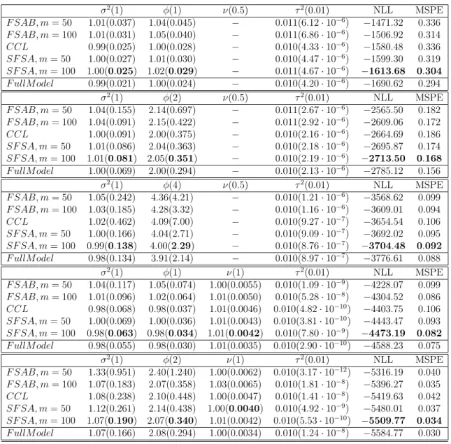
Compared with the approximated data covariance by the FSA-Block approach, the proposed method can correct part of the approximation errors across data blocks; compared with the approximated data covariance by the block conditional likelihood approach, the proposed method does not totally ignore the dependence among non-neighboring blocks and uses the covariance of predictive process model as approxi-mations. Therefore, the proposed method can induce a data covariance with smaller approximation errors. Figure 2.1 shows the absolute values of residual covariance matrix by three approaches, where the residual covariance isC_Y−C˜_Yfor some approx-imated data covariance matrix ˜C_Y. Specifically, 4000 locations are randomly selected in a square domain [0,10]×[0,10] and the exponential modelC(s,s0) = exp(−ks−s0k) with nugget effect 0.01 is evaluated on these locations. The grid is used to create blocks and block numbers are in an increasing order from northwest to southeast. The locations within the same block are grouped together and the neighboring set is

Sk−1 for Sk. Compared with the FSA-Block approach, since the residual covariance

between each block and its neighbors are corrected for the proposed method, we can observe that the entries of residual covariance matrix within a certain band are much smaller than those by the FSA-Block approach; compared with the conditional likelihood approach, while both methods provide good approximations for the covari-ance within blocks and between each block and its neighboring blocks, the proposed method leads to smaller entries of the residual covariance across blocks that are not neighbors due to including the covariance of the predictive process model.

(29)

Residual covariance 500 1000 1500 2000 2500 3000 3500 4000 500 1000 1500 2000 2500 3000 3500 4000 0 0.1 0.2 0.3 0.4 0.5 0.6 0.7 0.8 0.9

(a) The proposed method,K= 16

Residual covariance 500 1000 1500 2000 2500 3000 3500 4000 500 1000 1500 2000 2500 3000 3500 4000 0.1 0.2 0.3 0.4 0.5 0.6 0.7 0.8 0.9

(b) The proposed method,K= 100

(c) The FSA-Block approach,K= 16

Residual covariance 500 1000 1500 2000 2500 3000 3500 4000 500 1000 1500 2000 2500 3000 3500 4000 0.1 0.2 0.3 0.4 0.5 0.6 0.7 0.8 0.9

(d) The FSA-Block approach,K= 100

(e) The CCL approach,K= 16

Residual covariance 500 1000 1500 2000 2500 3000 3500 4000 500 1000 1500 2000 2500 3000 3500 4000 0.1 0.2 0.3 0.4 0.5 0.6 0.7 0.8 0.9 (f) The CCL approach,K= 100

Figure 2.1: Plots of residual covariance for 3 methods.

2.2.5 Computational complexity of the SFSA approach

(30)

proach needs to compute the quadratic term_YT_BT_(Σ−1 con−Σ −1 conBUΣw∗UTBTΣ−1 con)BY, where Σw∗ = (UTBTΣ−1 conBU+C −1

∗ )−1. The computation bottlenecks lie in

computa-tions of Σ−1

con, BU, andUTBTΣ −1

conBU. Since Σcon is block-diagonal, its inverse takes

O(Kn3

b) = O(nn2b) flops. BU has computational complexity O(nmqnb), because B

is a lower-triangular matrix with at mostqnb nonzero entries per row andU is anby

m matrix. The computation of UTBTΣ−_con1BU involves a product of am×n matrix and a n×m matrix, so its computation complexity isO(nm2). Therefore, the com-putational complexity of the proposed method has the orderO(nn2_b+nmqnb+nm2).

If we set the knot sizem n, the block sizenb n, andq K, then the proposed

method has computational complexity linear with n. 2.2.6 Choices of tuning parameters

The FSA-Block approach needs to specify the knot set and a block partition; compared with the FSA-Block approach, the proposed SFSA approach has additional tuning parameters: ordering of blocks and number of neighboring blocks q. For knots selection, a heuristic way is to predetermine the knot number according to the balance of available computing resources and pilot studies of statistical efficiency, then to place the knots with a good space coverage. For example, we can use random sampling, Latin Hypercube Sampling [52] or a spatial grid for placing the knots. Alternatively, we can treat the knots as model parameters and select them adaptively [34, 41, 78]. For the block partition, the goal is to maximize block numbers while minimizing the residual correlations across blocks. [19] provides some guidance on blocking strategy, and one recommendation is to use the empirical variogram to determine the block width. If the residual covariance is fairly isotropic, the partition algorithm based on Euclidean distances of locations such as K-means clustering is a simple choice. Unfortunately, since the predictive process covariance is not isotropic,

(31)

the residual covariance function is not isotropic too. In this case, applying clustering algorithm using the estimated residual covariance may be a better choice for block partition, but we stick to K-means clustering algorithm in this paper for its simplicity. The ordering of blocks can also affect the performance of the SFSA approach. Since the neighbors of one block can only be the past blocks (blocks with a smaller block number), the choices of neighbors are more restricted for blocks of a relatively small block number. So it may gain better statistical efficiency if we guarantee that a block of a small block number has some really close past blocks (the closeness of two blocks is measured by the distance of block centers). one heuristic way for ordering blocks is first to number a block with the minimum distance to all other blocks S1,

then number its nearest neighboring blockS2; given a current set of numbered blocks S(k) ₌_{_S

1, S2, . . . , Sk}, the block in the remaining blocks with the minimum distance

to the set S(k) is numbered Sk+1 and let S(k+1) ={S(k), Sk+1}; we keep ordering the

blocks until k = K. When the spatial locations are irregularly spaced such as the real dataset in Section 2.5, this heuristic ordering approach empirically works well. In Section 2.4, we illustrate the effect of number of neighboring blocks q. Based on the simulation results, a small number of neighboring blocks such as q = 4 (with several hundred neighboring observations) usually leads to performance very close to the full covariance model in terms of parameter estimation.

2.3 Parameter Estimation and Prediction 2.3.1 Maximum likelihood estimators

The maximum likelihood estimates of model parameters maximize the log-likelihood function (2.3). To facilitate computations, we replace the full covarianceC_Ywith the

(32)

approximated covariance C† Y in Theorem 2.2.1, `(_Y|θ,β) = −1 2|C † Y| − 1 2(Y−Xβ) T_C†−1 Y (Y−Xβ) + constant.

By the proof in Appendix,

C†−1 Y = Σ −1 con−Σ −1 conBUΣw∗UTBTΣ−1 con,

where Σw∗ = (UTBTΣ−_con1BU +C_∗−1)−1 is a m×m matrix, Σ_con is a block-diagonal

matrix and B is a sparse lower-triangular matrix. So the computations C_Y†−1 can be greatly reduced when we choose the knot size m, the block size nB, and number of

neighboring blocks q to be small. For the determinant,

|C† Y|=|U T_BT_Σ−1 conBU +C −1 ∗ | · |Σcon| · |C∗|.

Efficient computations can be achieved since we only need to compute the determi-nants of two m×m matrices and a block-diagonal matrix.

2.3.2 Bayesian inference on model parameters

The Bayesian inference starts from the specifications of prior distributions of β and θ. The conjugate normal prior π(β) ∼ N(µ0,Σ0) can be assigned to β.

The priors of θ depends on the form of the covariance function. Take the Mat´ern covariance model (2.2) as an example, the inverse gamma prior IG(a, b) can be assigned to variance parameterσ2 and the nuggetτ2where hyper-parametersa, bare chosen with guesses of the mean and variance; for the dependence range parameter, a uniform prior with a reasonable support of practical dependence ranges can be used; for smoothness parameter ν, usually an uniform prior at (0,2] is used since

(33)

high-order smoothness can hardly be identified for the real datasets.

We draw posterior samples of model parameters from the posterior p(β,θ|_Y) ∝

p(_Y|β,θ)π(β)π(θ). The full conditional distribution ofβhas a closed-formp(β|_Y,θ)∼ N(µβ|·,Σβ|·), where

µβ|· = Σβ|·(XTC_Y−1Y+ Σ−01µ0),

Σβ|· = (XTC_Y−1X+ Σ−₀1)−1.

The Gibbs sampler is used to draw posterior samples fromN(µβ|·,Σβ|·). Since the full

conditional distributions of θ don’t have closed-forms, we use Metropolis-Hastings algorithm to draw posterior samples of θ. For very large sample size n, we replace C_Y with the approximated covariance C†

Y by the SFSA approach in µβ|·,Σβ|·, and

p(_Y|β,θ), for obtaining posterior samples of model parameters. 2.3.3 Prediction

LetSp ={s1, . . . ,snp}be a set of predictive spatial locations such thatSp∩S =∅

and Yp = (Y(s1), . . . , Y(snp))

T _{be the corresponding vector of responses. Given the}

partition ruleP that partitionsS intoK blocks, suppose it partitionsSp intor ≤K

distinct blocks Sp,k with the block numberMk,k = 1, . . . , r. We start from the joint

densityp(Yp,_Y|β,θ) =R p(Yp|_Y,w∗,β,θ)·p(_Y|w∗,β,θ)·p(w∗|θ)dw∗. LetYp,k be the response vector at Sp,k, we define

˜ p(Yp|Y,w∗,β,θ) = r Y k=1 ˜ p(Yp,k|Y,w∗,β,θ) = r Y k=1 p(Yp,k|YMk,YN(Mk),w ∗ ,β,θ). (2.6)

(34)

This definition assumesYp,k’s are conditional independent givenw∗ and their

neigh-bors in _Y. By (2.6), the approximated joint density

where ˜p(_Y|w∗,β,θ) is the Gaussian density in (2.4). Then the approximated condi-tional density of Yp|Y,β,θ can be directly derived from ˜p(Yp,Y|β,θ).

Theorem 2.3.1. LetXpk denote the design matrix ofYp,k,Upk denoteC(Sp,k, S

∗_)C−1

∗

andΣ(pk)

con be the residual conditional variance ofYp,k, given its neighborsYN(Mk) and

YMk. DefineBpk = (Bpk,1, . . . , Bpk,K), where Bpk,l, l= 1, . . . , K has the same

defini-tion as (2.5). Let Xp = (XTp1, . . . ,X T pr) T_, _U p = (UpT1, . . . , U T pr) T_, _B p = (Bp1, . . . , Bpr) and Σp con = diag{Σ (p1)

con, . . . ,Σ(conpr)}, then the approximated conditional density Yp|Y,β,θ ∼ N(µp,Σp), where µ_p = Xpβ+FpC †−1 Y (Y−Xβ), Σp = Σpcon+BpB−1ΣconBT −1 BT_p +UpC∗UpT −FpC †−1 Y F T p , Fp = (−BpB−1ΣconBT −1 +UpC∗UT).

The conditional mean µ_p is the kriging formula for spatial predictions under the SFSA approximations. We postpone the proof of Theorem 2.3.1 to the next subsection 2.3.4 where we prove that the SFSA approach can induce a valid Gaussian process with a closed-form covariance function.

(35)

2.3.4 The Smooth FSA spatial process

Actually the SFSA approach can yield a valid spatial process so that both the parameter estimation and prediction can be performed in the same framework. In Section 2.2.2, we show that the underlying spatial process w(s) can be decom-posed into two independent processes wl(s) and ws(s), where wl(s) is the

predic-tive process with covariance function Cl(·,·) and ws(s) is the exact residual

pro-cess with covariance function C(·,·) − Cl(·,·). Let ˜ws(s) = ws(s) + (s) be the

new residual process incorporating the nugget effect, then the data process Y(s) =

xT₍_s_)β₊_w

l(s) + ˜ws(s). In the following we show that the proposed method

approx-imates the exact residual process ˜ws(s) by a block version of the nearest neighboring

process [18]. Given a partition rule P leading to S = ∪K

k=1Sk, the key assumption

˜

p(_Y|β,θ,w∗) =

K

Q

k=1

p(Yk|YN(k),β,θ,w∗) of the proposed approach is equivalent to

˜

p( ˜ws(S)|θ) = K

Q

k=1

p( ˜ws(Sk)|w˜s(SN(k)),θ), since ˜ws(s) is the only random component

given w∗ and all model parameters. Thus for the SFSA approach, a block ver-sion of the nearest neighboring approximation is applied to the residual likelihood

p( ˜ws(S)|θ). Following the results in [18], the resulting approximated residual

covari-ance matrix is B−1_Σ

conBT −1

, denoted by Σ†

Y.

Let P partitions a set of predictive locations Sp into r distinct blocks Sp,k and

denote the block number of Sp,k byMk,k = 1, . . . , r. We assume that

˜ p( ˜ws(Sp)|w˜s(S),θ) = r Y k=1 p( ˜ws(Sp,k)|w˜s(SMk),w˜s(SN(Mk)),θ).

This assumption is equivalent to ˜p(Yp|Y,w∗,θ) = r

Q

k=1

p(Yp,k|YMk,YN(Mk),w

∗_,_{θ) in}

(36)

predictive location set in Sv. Denote ˜ws(Sv) by ˜wv and ˜ws(Su) by ˜wu, we define ˜ p( ˜wv|θ) = Z ˜ p( ˜wu|w˜s(S),θ)˜p( ˜ws(S)|θ) Y si∈S\Sv dw˜s(si). (2.7)

It is easy to verify that the defined residual process, denoted by ˜w†_s(s), satisfies the conditions of Kolmogorov consistency theorem and is a valid spatial process [18]. According to the law of total covariance

Cov( ˜w_s†(s),w˜†_s(s0)) = E(Cov( ˜w†_s(s),w˜†_s(s0)|w˜s(S)))+Cov(E( ˜w†s(s)|w˜s(S)),E( ˜ws†(s 0_)|

˜

ws(S))),

the covariance function of ˜w†_s(s) is

˜ C_s†(s,s0) =                  Σ† Y(s,s 0₎_, _if _s_,_s0 _∈_S_; −BsΣ † Y(S,s 0₎_, _if _s_∈_/ _S, _s0 _∈_S_; BsΣ † YB T

s0, if s,s0 ∈/ S, s,s0 belong to different blocks; BsΣ † YB T s0 + Σ (pk)

con(s,s0), if s,s0 ∈/ S, s,s0 belong to the same blockpk,

where Σ†

Y(S1, S2) and Σ

(pk)

con(S1, S2) denote the sub-matrices of Σ

†

Y and Σ

(pk)

con

corre-sponding to the covariance of location sets S1 and S2, respectively. The covariance

function of the data process by the SFSA approach is

C†(s,s0) =Cl(s,s0) + ˜Cs†(s,s 0

).

So the approximated cross covariance between the predictive set Sp and the training

set S is UpC∗UT −BpΣ †

Y and the kriging formula yields the conditional mean of

Yp given Y in Theorem 2.3.1. The conditional variance in Theorem 2.3.1 can be

(37)

2.4 Simulation Study

In this section, we illustrate the effectiveness of our method through simulation studies and a precipitation dataset. The implementations of all methods are written in Matlab and run on a processor with 2.9 GHz Xeon CPUs and 16GB memory. For likelihood function optimization, we use the matlab function fminunc which imple-ments a Broyden-Fletcher-Goldfarb-Shanno (BFGS) based Quasi-Newton method. 2.4.1 Prediction in spatial holes

Consider 4000 locations randomly selected in the spatial domain S = [0,10]× [0,10]. We held out 208 locations in the rectangular regions [1.5,3.5]×[1.5,2.5] and [6.5,8.5]×[6.5,7.5] as the predictive locations, and the rest of locations were used as training locations. This prediction scenario mimics the missing pattern of the satellite datasets where missing data are usually due to sizable holes. We generate realizations of Y(s) from the model (3.1) with β = 0 and the Mat´ern covariance model (2.2). A nugget effect τ2 _{is added to covariance model (2.2) accounting for}

the measurement errors of responses. We compare the proposed method (denoted by “SFSA”) with the FSA-Block approach (denoted by “FSAB”), and the block version of the conditional likelihood approximation approach in [18] (denoted by “CCL”) in terms of parameter estimation and prediction results. The full covariance model results (denoted by “FullModel”) serve as the baseline. All three methods require a partition of the observed dataset, and the SFSA and CCL approaches also need an ordering of data blocks. In this simulation study, the regular grid block centers are created for the block partition and the block numbers are sorted in an increasing order from northwest corner to southeast corner. For the SFSA and the FSA-Block approaches, we randomly select m = 50,100 knot locations inS. For the SFSA and the CCL approaches, we consider using the nearest block (q= 1) in the past blocks

(38)

as the neighbor of each block. The Maximum Likelihood Estimates (MLEs) of model parameters are calculated based on the training set and the Mean Squared Prediction Errors (MSPEs) are computed for the prediction set. The Negative Log-Likelihood values (NLL) up to a constant n₂ log(2π) are also obtained as a measure of model fitting. We experiment different parameter values of the covariance model (2.2) and the results are shown in Table 2.1.

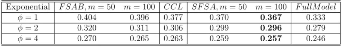
In terms of parameter estimation, the SFSA always produces close means and Mean Squared Errors (MSE) to the full model results for covariance parameters un-der different dependence range scenarios. For the exponential model ν = 0.5, when the dependence range is relatively small, both the SFSA and the CCL methods have smaller MSEs than that by the FSA-Block approach, this is because the predictive process component of the FSA-Block approach doesn’t give an adequate approxima-tion to the dependence across blocks, and the loss of informaapproxima-tion is relatively severe under the small-scale dependence scenario; when the dependence range is relatively large such asφ = 4, both the SFSA and the FSA-Block outperform the CCL method, since the correlations across blocks are not negligible. In this case, the predictive process component does a good job in approximating the cross-block dependence, so the SFSA and the FSA-Block can produce smaller MSEs of model parameters. We remark that the SFSA approach produces smaller MSEs and NLLs than that by the FSA-Block approach in all 3 dependence range cases for the exponential model, due to the additional corrections of correlations among neighboring blocks. In addition, the parameter estimation results of the SFSA approach are less sensitive to the knot numbers compared to the FSA-Block approach. For the Mat´ern covariance mod-el with ν = 1, we have similar observations to the exponential model case. When the knot number is small (m = 50), the FSA-Block approach yields significantly larger MSEs than that of the SFSA method for parameters σ2 _and _φ_{; the proposed}

(39)

Table 2.1: Means and Mean Squared Errors (in parenthesis) of parameters in Mat´ern covariance model. The number of blocks K = 100 for all three methods and the results are based on 200 simulated datasets.

σ2₍₁₎ _φ₍₁₎ _ν₍₀_.₅₎ _τ2₍₀_.₀₁₎ _NLL _MSPE F SAB, m= 50 1.01(0.037) 1.04(0.045) − 0.011(6.12·10−6₎ ₋₁₄₇₁_.₃₂ ₀_.₃₃₆ F SAB, m= 100 1.01(0.031) 1.05(0.040) − 0.011(6.86·10−6₎ ₋₁₅₀₆_.₉₂ ₀_.₃₁₄ CCL 0.99(0.025) 1.00(0.028) − 0.010(4.33·10−6₎ ₋₁₅₈₀_.₄₈ ₀_.₃₃₆ SF SA, m= 50 1.00(0.027) 1.01(0.030) − 0.010(4.47·10−6₎ ₋₁₅₉₉_.₃₀ ₀_.₃₁₉ SF SA, m= 100 1.00(0.025) 1.02(0.029) − 0.011(4.67·10−6₎ ₋₁₆₁₃_.₆₈ ₀_.₃₀₄ F ullM odel 0.99(0.021) 1.00(0.024) − 0.010(4.20·10−6₎ ₋₁₆₉₀_.₆₂ ₀_.₂₉₄ σ2₍₁₎ _φ₍₂₎ _ν₍₀_.₅₎ _τ2₍₀_.₀₁₎ _NLL _MSPE F SAB, m= 50 1.04(0.155) 2.14(0.697) − 0.011(2.67·10−6₎ ₋₂₅₆₅_.₅₀ ₀_.₁₈₂ F SAB, m= 100 1.04(0.091) 2.15(0.422) − 0.011(2.92·10−6₎ ₋₂₆₀₉_.₀₆ ₀_.₁₇₂ CCL 1.00(0.091) 2.00(0.375) − 0.010(2.16·10−6₎ ₋₂₆₆₄_.₆₉ ₀_.₁₈₆ SF SA, m= 50 1.01(0.086) 2.04(0.363) − 0.010(2.18·10−6₎ ₋₂₆₉₅_.₈₇ ₀_.₁₇₄ SF SA, m= 100 1.01(0.081) 2.05(0.351) − 0.010(2.19·10−6₎ ₋₂₇₁₃_.₅₀ ₀_.₁₆₈ F ullM odel 1.00(0.069) 2.00(0.294) − 0.010(2.13·10−6₎ ₋₂₇₈₅_.₁₂ ₀_.₁₅₆ σ2₍₁₎ _φ₍₄₎ _ν₍₀_.₅₎ _τ2₍₀_.₀₁₎ _NLL _MSPE F SAB, m= 50 1.05(0.242) 4.36(4.21) − 0.010(1.21·10−6₎ ₋₃₅₆₈_.₆₂ ₀_.₀₉₉ F SAB, m= 100 1.03(0.185) 4.28(3.32) − 0.010(1.16·10−6₎ −3609.01 0.094 CCL 1.02(0.462) 4.09(7.00) − 0.010(9.27·10−7₎ ₋₃₆₅₄_.₅₄ ₀_.₁₀₆ SF SA, m= 50 1.00(0.166) 4.04(2.71) − 0.010(9.09·10−7₎ ₋₃₆₉₂_.₀₂ ₀_.₀₉₅ SF SA, m= 100 0.99(0.138) 4.00(2.29) − 0.010(8.76·10−7₎ −3704.48 0.092 F ullM odel 0.98(0.134) 3.91(2.14) − 0.010(8.97·10−7₎ ₋₃₇₇₆_.₆₁ ₀_.₀₈₈ σ2₍₁₎ _φ₍₁₎ _ν₍₁₎ _τ2₍₀_.₀₁₎ _NLL _MSPE F SAB, m= 50 1.04(0.117) 1.05(0.074) 1.00(0.0055) 0.010(1.09·10−9₎ ₋₄₂₂₈_.₀₇ ₀_.₀₉₉ F SAB, m= 100 1.01(0.096) 1.02(0.064) 1.01(0.0050) 0.010(5.28·10−8₎ ₋₄₃₀₄_.₅₂ ₀_.₀₈₆ CCL 0.98(0.068) 0.98(0.037) 1.01(0.0046) 0.010(4.82·10−10₎ ₋₄₄₀₃_.₇₅ ₀_.₁₀₆ SF SA, m= 50 1.00(0.069) 1.00(0.036) 1.01(0.0043) 0.010(3.81·10−10₎ ₋₄₄₄₃_.₄₇ ₀_.₀₉₃ SF SA, m= 100 0.98(0.063) 0.98(0.034) 1.01(0.0042) 0.010(7.80·10−9₎ ₋₄₄₇₃_.₁₉ ₀_.₀₈₂ F ullM odel 0.98(0.055) 0.98(0.030) 1.01(0.0035) 0.010(2.90·10−10₎ ₋₄₅₈₈_.₂₃ ₀_.₀₇₅ σ2₍₁₎ _φ₍₂₎ _ν₍₁₎ _τ2₍₀_.₀₁₎ _NLL _MSPE F SAB, m= 50 1.33(0.951) 2.40(1.240) 1.00(0.0062) 0.010(3.17·10−12₎ −5316.19 0.040 F SAB, m= 100 1.07(0.183) 2.07(0.358) 1.03(0.0065) 0.010(1.81·10−8₎ ₋₅₃₉₆_.₂₇ ₀_.₀₃₅ CCL 1.08(0.238) 2.10(0.448) 1.00(0.0047) 0.010(1.41·10−8₎ ₋₅₄₁₉_.₆₃ ₀_.₀₄₂ SF SA, m= 50 1.12(0.261) 2.14(0.438) 1.00(0.0040) 0.010(4.92·10−9₎ −5480.01 0.037 SF SA, m= 100 1.07(0.190) 2.07(0.340) 1.01(0.0042) 0.010(5.53·10−10₎ ₋₅₅₀₉_.₇₇ ₀_.₀₃₄ F ullM odel 1.07(0.166) 2.08(0.294) 1.00(0.0034) 0.010(1.24·10−8₎ ₋₅₅₈₄_.₇₇ ₀_.₀₃₀

method produces similar MSEs of parameters for different knot numbers, indicating its insensitiveness to the knot number.

In terms of prediction, the SFSA and FSA-Block approach outperform the CCL approach in all scenarios, this may be because the knot-based approaches can gain

(40)

Table 2.2: MSPEs and MSEs of the exponential model with sample size 4000. The number of blocks K = 100. σ2₍₁₎ _φ₍₁₎ _τ2₍₀_.₂₎ _NLL _MSPE F SAB, m= 50 1.00(0.035) 1.07(0.066) 0.204(1.45·10−4₎ ₂₉₂_.₉₃ ₀_.₅₇₅ F SAB, m= 100 1.00(0.032) 1.09(0.062) 0.205(1.39·10−4₎ ₂₇₁_.₂₆ ₀_.₅₅₂ CCL 0.99(0.029) 0.99(0.043) 0.198(1.16·10−4₎ ₂₄₃_.₄₄ ₀_.₅₇₃ SF SA, m= 50 0.98(0.026) 1.00(0.041) 0.200(1.13·10−4₎ ₂₂₄_.₆₀ ₀_.₅₆₃ SF SA, m= 100 0.99(0.026) 1.02(0.041) 0.201(1.11·10−4₎ ₂₁₆_.₈₁ ₀_.₅₄₄ F ullM odel 0.98(0.025) 0.98(0.035) 0.199(1.0·10−4₎ ₁₇₄_.₃₉ ₀_.₅₂₅ σ2₍₁₎ _φ₍₂₎ _τ2₍₀_.₂₎ _NLL _MSPE F SAB, m= 50 1.09(0.219) 2.43(1.460) 0.204(7.67·10−5₎ ₋₁₅₀_.₇₄ ₀_.₄₁₀ F SAB, m= 100 1.07(0.141) 2.40(0.993) 0.204(7.20·10−5₎ ₋₁₈₁_.₇₅ ₀_.₃₉₈ CCL 0.98(0.088) 1.99(0.423) 0.199(5.78·10−5₎ ₋₁₈₄_.₀₀ ₀_.₄₁₉ SF SA, m= 50 1.02(0.102) 2.13(0.552) 0.201(5.61·10−5₎ ₋₂₁₀_.₅₁ ₀_.₄₀₄ SF SA, m= 100 1.01(0.080) 2.12(0.446) 0.201(5.50·10−5₎ ₋₂₂₃_.₀₅ ₀_.₃₉₃ F ullM odel 0.98(0.072) 1.98(0.354) 0.199(5.38·10−5₎ ₋₂₅₂_.₈₁ ₀_.₃₇₇ σ2₍₁₎ _φ₍₄₎ _τ2₍₀_.₂₎ _NLL _MSPE F SAB, m= 50 1.15(0.518) 5.25(12.30) 0.202(5.26·10−5₎ −481.89 0.316 F SAB, m= 100 1.02(0.179) 4.60(4.03) 0.202(4.79·10−5₎ ₋₅₁₂_.₄₈ ₀_.₃₀₉ CCL 0.94(0.275) 3.8(4.82) 0.198(5.04·10−5₎ ₋₄₉₉_.₉₅ ₀_.₃₂₄ SF SA, m= 50 0.99(0.214) 4.18(3.80) 0.200(4.39·10−5₎ −528.58 0.311 SF SA, m= 100 0.96(0.150) 4.07(2.72) 0.200(4.37·10−5₎ ₋₅₃₈_.₉₃ ₀_.₃₀₅ F ullM odel 0.93(0.131) 3.74(2.24) 0.198(4.45·10−5₎ ₋₅₆₁_.₉₂ ₀_.₃₀₀

additional information for the predictive locations in the spatial hole when we place knots around or in the spatial hole. The prediction errors of all 3 methods decrease with the increase of dependence range parameter φ, since more information can be borrowed from the training set under the large scale dependence structure. Compared with the FSA-Block approach with equal number of knots, the SFSA has smaller MSPEs due to additional corrections of correlations across blocks. The prediction difference between SFSA and FSA-Block is relatively larger when the dependence scale is small and the process is less smooth, since in this case, the predictive process component of the FSA-Block doesn’t perform well in approximating the correlations across blocks. Table 2.2 shows the parameter estimation and prediction results when the data is generated with a high noise level 0.2. The observations are similar to the simulation set-up with a low noise level 0.01.

(41)

# of neighbors 0 2 4 6 8 10 MSE 0.02 0.022 0.024 0.026 0.028 MSE of sigma2 SFSA Full Model # of neighbors 0 2 4 6 8 10 MSE 0.022 0.024 0.026 0.028 0.03 MSE of beta SFSA Full Model # of neighbors 0 2 4 6 8 10 MSE ×10-6 4.1 4.2 4.3 4.4 4.5 MSE of epsilon SFSA Full Model # of neighbors 0 2 4 6 8 10 NLL -1700 -1650 -1600 -1550 NLL SFSA Full Model

Figure 2.2: MSE of each covariance parameter against the number of neighboring blocks for the SFSA approach. The simulation setting is the same as that described in Section 2.4.1; the covariance model is exponential model with φ = 1, σ2 _{= 1, and} τ2 = 0.01.

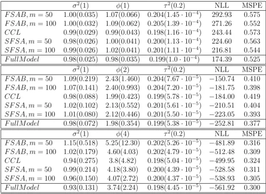
Figure 2.2 shows how the MSEs and NLL change with the number of neighboring blocks for the SFSA approach. Whenq ≥4, the SFSA approach can produce results almost at par with the full covariance model. Notice that the neighboring locations of a block for q = 4 is only about 200, so the proposed method can achieve good parameter estimation results at very low costs of computations. For predictions, figure 2.3 shows how the MSPEs change with number of neighboring blocks. We find that the prediction performance is more sensitive to the block size than to the number of neighbors for the prediction in spatial hole scenario. This may be because for the grid partition, each spatial hole covers more than one block when we choose

(42)

not have enough nearby locations due to the block ordering. Thus when we partition the data into small number of blocks, the prediction error drops more significantly due to the increased number of very close locations in the neighbor set.

# of neighbors 2 4 6 8 10 MSPE 0.29 0.3 0.31 0.32 0.33 MSPE, K=100 SFSA Full Model # of neighbors 1 2 3 4 5 MSPE 0.29 0.3 0.31 0.32 0.33 MSPE, K=25 SFSA Full Model

Figure 2.3: MSPEs against the number of neighboring blocks for the SFSA approach with K = 25,100. The simulation setting is the same as that described in Section 2.4.1; the covariance model is exponential model with φ= 1, σ2 _{= 1, and} _τ2 _{= 0}_._01.

2.4.2 Prediction on block boundaries

For the FSA-Block approach, when predicting responses on shared boundaries of two blocks, the prediction of a boundary location depends on which block it belongs to. Although the FSA-Block approach has the predictive process part as the “global” support, the discontinuity caused by the independent blocks approximation of the residual covariance can be severe when the predictive process component does not perform well due to limited knot number. Since the proposed approach takes the neighboring blocks information into account for modeling the residual process, we expect that it can produce a smoother prediction surface than that by the FSA-Block approach. Compared with the conditional likelihood approximation method [18], it may also relieve the discontinuity problem for predicting on boundary locations