Taxes or Fees? The Political Economy of Providing Excludable Public Goods

A joint Initiative of Ludwig-Maximilians-Universität and Ifo Institute for Economic Research

Working Papers

August 2001

CESifo

Center for Economic Studies & Ifo Institute for Economic Research Poschingerstr. 5, 81679 Munich, Germany

Phone: +49 (89) 9224-1410 - Fax: +49 (89) 9224-1409 e-mail: office@CESifo.de

ISSN 1617-9595

!

An electronic version of the paper may be downloaded • from the SSRN website: www.SSRN.com

• from the CESifo website: www.CESifo.de

TAXES OR FEES?

THE POLITICAL ECONOMY OF PROVIDING

EXCLUDABLE PUBLIC GOODS

Kurtis J. Swope

Eckhard Janeba

CESifo

Working Paper No. 542

August 2001

TAXES OR FEES?

THE POLITICAL ECONOMY OF PROVIDING

EXCLUDABLE PUBLIC GOODS

Abstract

This paper provides a positive analysis of public provision of excludable public goods financed by uniform taxes or fees. Individuals differing in preferences decide using majority-rule the provision level and financing instrument. The median preference individual is the decisive voter in a tax regime, while an individual with preferences above the median generally determines the fee in a fee regime. Numerical solutions indicate that populations with uniform or left-skewed distributions of preferences choose taxes, while a majority coalition of high and low preference individuals prefer fees when preferences are sufficiently right-skewed. Public good provision under fees exceeds that under taxes in the latter case.

Keywords: excludable public goods, public provision, voting. JEL Classification: P26, H41. Kurtis J. Swope Department of Economics U.S.Naval Academy 589 McNair Rd. Stop 10 D Annapolis, MD 21402 U.S.A. Swope@usna.edu Eckhard Janeba University of Colorado Economics Department Campus Box 256 Boulder, CO 80309 U.S.A.

1. Introduction

Many excludable public goods are provided by the state. Examples in the U.S. include national, state, and local parks, state and federal wildlife programs that stock and monitor fish and game for sportsmen, and outdoor recreation areas for hiking, backpacking, bicycling, or cross-country skiing. In Europe, reception of public television broadcasts requires households to purchase a license. Issues related to both the level of provision and financing method are increasingly the subject of public debate because the possibility of exclusion permits both tax-based provision and fee-tax-based provision by the state.1 Under tax-based provision, all individuals

pay through taxes. Once the good is provided, all individuals may consume the good at no additional charge. Under fee-based provision of public goods, individuals may opt out and pay no fee, but are then excluded from consuming the good.

From a normative standpoint exclusion of individuals under a fee-based system indicates an inefficiency if the marginal cost of additional consumers is zero. Whether taxes are superior or not, however, depends also on the level of the provision under each regime and the progressivity of the financing. Fraser (1996) therefore considers the welfare ranking of tax versus fee-based public provision regimes for an excludable public good. He shows that when governments set the fee or tax to maximize utilitarian social welfare, the good is underprovided under fees relative to tax-based provision. Often, however, we observe that fee-based financing schemes find strong public support, even from those who are most likely the consumers. Consider the recent statement by Derrick Crandall, President of the American Recreation Coalition (ARC), to the U.S. Senate Committee on Energy and Natural Resources:

1

For example, compare the positive response of Fretwell (1999) and Crandall (in U.S. Senate, 1999) to increased use of fees by the U.S. National Park Service to the negative response of a number of other organizations. A list of organizations opposed to the fees can be found at http://www.freeourforests.org/opposition.html.

We perceive fees as one element in assuring the public that their visits to their lands will be enjoyable and safe. The recreation community enjoys free lunches just as much as any other interest group, but we have come to understand that it is hard to demand a great meal when you aren't paying. And we certainly understand that quality recreation on federal lands really isn't a free lunch: the costs have simply been borne by general taxes, not user fees. However, there is a real downside to that situation. We've seen that during recent periods of financial pressure on the federal government, recreation programs are placed in jeopardy…Americans across the country made clear that they were willing to pay reasonable fees for quality recreation

opportunities -- just as they will pay reasonable costs for quality sleeping bags and boats. (U.S. Senate, 1999, p. 9)

The support for fees seems difficult to reconcile with the normative perspective. In this paper we consider a political economy approach to explain this stylized fact. In contrast to Fraser, we show that when the financing instrument and level of provision are chosen through majority-rule voting, fees can provide a higher level of the public good relative to taxes in some cases. Furthermore, fees may be preferred by a majority of individuals in these cases.

The main logic behind these findings derives from the insight that individuals with strong preferences for the good prefer and vote for higher fees or taxes than individuals with low preferences. If tax financing is chosen, strong preference individuals face resistance from all low-preference individuals to an increase in the tax rate because everyone has to pay a tax. Thus, the equilibrium tax can be no higher than that most preferred by the individual with the median preferences. However, because low-preference individuals have the ability to opt out under fees, they become indifferent over marginal changes in a fee if the current level already exceeds their maximum willingness to pay. Therefore, some low preference individuals abstain from voting over increases. Hence, strong preference individuals face less opposition to fee increases than tax increases. This explains how the equilibrium fee can be higher than the fee most preferred by the individual with the median preferences. In addition, low-preference individuals may vote

The latter result depends on the overall distribution of preferences. We use numerical techniques to gain further insight. When preferences are distributed uniformly or are left-skewed, implying a population where most individuals have relatively strong preferences for the good, a majority of individuals prefers tax-based provision. When preferences are right-skewed, the majority may prefer fee-based provision. The level of public good provision under fee financing is lower relative to tax financing when the distribution of preferences is uniform or left-skewed, but may exceed that under tax financing when the distribution of preferences is right-skewed. While our main focus is to analyze the provision from a positive viewpoint, we also rank political and welfare maximization outcomes in terms of utilitarian welfare.

Our analysis builds on several previous works. A vast literature on club theory, as introduced by Buchanan (1965), focuses on the potential for excludable public goods to be efficiently provided by a private, decentralized, competitive network of clubs. Brito and Oakland (1980) examine the question of private market provision of an excludable public good under conditions of a monopoly and find that a monopoly leads to underprovision relative to the socially optimal level. Our analysis differs from the club literature by considering goods for which natural, locational, or jurisdictional barriers prevent free entry by potential providers. For example, Yellowstone National Park has unique factors of production that are not readily available to potential competitors. Although the analysis considers a single provider, it differs from that of Brito and Oakland because it is primarily concerned with those goods that are publicly rather than privately provided, and, therefore, can potentially be funded by taxes as well as fees.

Our work has a clear link to the literature on public versus private provision of education. Most of these papers consider the ability of households to opt out of public education for a

private alternative when the level of public education is unsatisfactory. The ‘ends against the middle’ voting outcomes in Epple and Romano (1996) bear strong resemblance to voting outcomes derived here, but for significantly different reasons. In Epple and Romano, a coalition of high and low-income households opposes higher expenditures for public education, while middle-income households prefer higher expenditures. Low-income households oppose higher expenditures for public education because of the high opportunity cost of increased expenditures, while high-income households oppose higher expenditures because they prefer to opt out of public education for a higher quality private alternative. In the current analysis, low-preference individuals prefer fees to taxes because they can opt out under fees, while high-preference individuals may prefer fees to taxes when fees provide a higher quality of the public good than taxes. This can generate a similar ‘ends against the middle’ voting outcome.

Helsley and Strange (1998) examine the strategic interaction between a private government and the public sector. Private governments are “voluntary, exclusive organizations that supplement services provided by the public sector” (p. 281). Private governments form when a group of consumers is dissatisfied with the level of a public service being provided by the public sector. In the Helsley and Strange analysis, consumers determine the level of public good provision by supplementing public provision levels, while consumers in the current analysis determine the level of public good provision by choosing the form and level of public funding. Oakland (1972), Laux-Mieselbach (1988), and Silva and Kahn (1993) all address the degree and optimality of exclusion. Here, it is assumed that exclusion is perfect and costless to the providing agency.

individuals who prefer a fee regime to a tax regime. In section 4 we use specific functional forms to find out if and under what circumstances the people who favor a fee regime have a majority. Section 5 solves for the best tax and fee levels, and compares overall welfare under the first-best policy and the politically determined fee and tax. Section 6 concludes and discusses future research. Technical derivations are found in an appendix.

2. The Model

The basic model is adopted from Silva and Kahn (1993). A population of size one is a continuum of individuals who derive utility from a non-rival, excludable shared good, G, and a pure, composite, private, numeraire good, m. Each individual is endowed with m0 units of the numeraire. Individuals have heterogeneous preferences for the public good. The utility of a type θ individual that consumes m units of the private good and G units of the collective good is

) ( ) ; , (m G m v G U θ = +θ . (1)

The function v(G) is assumed to be smooth, strictly increasing, and strictly concave and is the same for all individuals. We also assume v(0)=0. Individual type θ is distributed with continuous, atomless distribution function F(θ)and density function f(θ)on the interval

] , [θθ

θ∈ with θ≥0and θ<θ<∞.

We consider two types of regimes for financing good G.2 In a tax regime each individual pays a tax t and private consumption is m0 – t. In the fee regime an individual who subscribes pays a fee s and spends the remainder on the private good. The budget constraint faced by each individual takes the form

2

To make our point as simple as possible, we consider only two easily implemented financing schemes. We abstract from more complicated revelation mechanisms that could be beneficial when information about preferences is incomplete.

fee, if tax if 0    − = s t m m δ (2)

whereδis an indicator variable which takes the value of 1 if the individual subscribes and 0 otherwise.

The public agency providing G is assumed to be non-profit and to have a balanced budget. The marginal cost of additional units of G is assumed to be constant, equal to 1, and known by everyone. Thus, recalling that the population is normalized to 1, the government budget constraint is of the form

   = fee, if tax if sn t G (3)

where nrepresents the fraction of the population that subscribes.

Through the political process society decides via majority rule whether a tax or fee regime is implemented and determines the level of the fee or tax. We can model this as a three-stage process. At Stage 1, individuals choose the method of financing provision of the public good, either through taxes or fees. At Stage 2 individuals choose the level of the tax or fee that is imposed. If fees were chosen at Stage 1, each individual also decides at Stage 3 whether or not to pay the fee and consume the public good, or spend his entire endowment on the private good. No decision has to be made under the tax regime in Stage 3.

The three-stage public choice process is solved using backward induction. We assume that all individuals vote sincerely, that is, at Stages 1 and 2 each individual votes for the policy that gives highest utility. In the remainder of this section, we solve for Stages 2 and 3 under both regimes.

2.1 Tax-based Provision

Under tax-based provision the public good is financed via a mandatory, non-negative, lump-sum head tax t∈[0,m₀] paid by all individuals in the population. The pool of consumers under a tax is the entire population. Furthermore, because utility from the public good is non-negative and consumption requires no additional cost to the individual, all individuals find it optimal to consume the good. Combining conditions (1)-(3), the utility of a type θ individual paying a tax of t is, therefore,

) ( ) ; (m₀ t m₀ t v t U − θ = − +θ . (4)

An individual’s most preferred tax rate depends on θ. Maximizing (4) with respect to the tax rate gives the most preferred tax rate

     > ≥ ≥ < = − θ θ θ θ θ / 1 ) ( ' if ) ( ' / 1 ) 0 ( ' if ) / 1 ( ' / 1 ) 0 ( ' if 0 ) ( 0 0 0 1 m v m m v v v v t (5)

Assuming for a moment that t(θ)is strictly between 0 and m₀, we find by differentiating the

middle branch of (5) that most preferred tax rates are an increasing function of θ,

( )

( )

( ) 0 ) ( ) ( > ′′ ′ − = ∂ ∂ θ θ θ θ θ t v t v t . (6)

The equilibrium tax te under majority-rule voting is the tax that defeats any alternative tax in a pairwise vote. Note that preferences over tax rates are single-peaked on the interval [0,m₀]

because (4) is strictly concave in t. Hence the median voter result can be invoked.3 This leads to the following result. In a tax regime, the equilibrium tax under majority-rule voting is the

tax most preferred by the individual with the median preferences _θm_{, i.e.}

) ( m e t t = θ . 3

2.2 Fee-based Provision

All individuals desiring access to the public good must pay a one-time subscription fee, s. Hereafter, we refer to individuals choosing to pay the fee and consume the good as subscribers. Non-subscribers are individuals who choose to opt out in the fee regime. We assume that access to the public good is characterized by imperfect or coarse exclusion (Helsley and Strange, 1991), which implies that subscribers cannot be charged differently based on their intensity of use or number of uses. The utility of a type θ individual under fee-based provision therefore is

)] ( , 0 max[ )] ( , max[ ) ; , , (m₀ s G m₀ m₀ s v G m₀ s v G U θ = − +θ = + − +θ (7)

We now wish to characterize the outcome in the third stage. The first step is to find the number of subscribers for arbitrary levels of the fee and public good. This requires identifying the marginal consumer who is just indifferent between subscribing and not subscribing. Note that utility in (7) is non-decreasing in θ and strictly increasing in θ when θv(G)>s. Therefore there exists a θˆ such that θˆ= s/v(G)and all θ≥θˆ subscribe. For G>0, the individual with type θˆ is the marginal consumer where,

     < ≤ ≤ > = ), ( / if ) ( / if ) ( / ) ( / if ) , ( ˆ G v s G v s G v s G v s G s θ θ θ θ θ θ θ (8)

and θˆ(s,0)=θ. All individuals with type θ≥θˆ choose to subscribe to the public good, while all individuals with type θ<θˆdo not subscribe. The supply of the public good depends on the fee s and the number of subscribers. For any levels of s and θˆ , the supply of the public good is

( )

s,θˆ s[1 F(θˆ)]

where n =[1−F(θˆ)]is the proportion of individuals with θ≥θˆ (i.e. those who choose to subscribe). For any fee s, conditions (8) and (9) simultaneously determine G and θˆ . Let the solution be G(s)and θˆ(s). The pair G(s)=0 and θˆ(s)=θ always satisfies (8) and (9) and hence a solution exists.

Without further assumptions the demonstration and characterization of an equilibrium fee under majority-rule voting is difficult due to the simultaneity of conditions (8) and (9). In the appendix we derive conditions for single-peakedness of preferences. We show also that there exists a simple necessary condition that characterizes the equilibrium fee. We discuss this condition below and check in our numerical analysis that an equilibrium indeed exists. We relegate the more technical derivation of these conditions to the appendix.

We should note an important assumption in our analysis. Consider a situation in which individuals vote over two different fees and some individuals would opt out under both. What is their voting behavior? We assume that these individuals abstain from voting, perhaps because of small but positive voting costs, or vote for either fee with probability one half. Other voting behavior could lead to different outcomes, but our assumption has intuitive appeal.

The necessary condition that an equilibrium fee s must satisfy is quite intuitive. The

number of people who prefer a fee higher than s must be equal to the number of people

who prefer a smaller fee and choose to pay s, that is, the equilibrium fee is the one chosen by the median of non-abstainers. This condition can be written as follows

(

( )

)

(

( )

)

( )

ˆ( )

1−F θ s = Fθ s −Fθ s , (10)

where θ(s) is the individual who most prefers s, and θˆ(s) is the marginal consumer type at s. Figure 1 presents the necessary condition for an equilibrium fee graphically. In the figure, θm

represents the overall median preference individual, but θ(s) represents the median of the subscribers at the fee s and satisfies (10).

Figure 1. The necessary condition for an equilibrium fee s

      → ←(i.e.−abstainers) s subscriber non                      → ← subscribers θ θˆ

( )

s θm θ(s) θ ←→ − (ˆ( )) )) ( ( s F s F θ θ ←1−F(θ(s))→

prefer a lower fee than s = prefer a higher fee than s

In the appendix we show that there always exists a fee that solves (10) and, if there are more than one, an equilibrium fee will be the smallest of all fees that fulfill (10).

Condition (10) is useful in characterizing the equilibrium. In fact, we can now state one insight that is readily apparent from Figure 1. If all individuals subscribe at the most

preferred fee by the individual with median preference, then the equilibrium fee is the one preferred by the median person. Otherwise the equilibrium fee, when one exists, is higher than the one preferred by the median person. This follows from (10).

We now turn to the main question of the analysis. Which of the two financing methods is chosen under majority voting?

3. Tax versus Fee: The Equilibrium Policy Choice

stage as a basis for voting for fees or taxes in the first stage. An important result follows now from the previous section. When the person with median preference is the decisive voter in

the fee regime, then the fee and the tax are the same, provide the same level of the public

good, and all individuals subscribe, i.e., _se _=s m _=t m _=te

) ( )

(θ θ and G(se)=G(te). This

result holds because under the fee the equilibrium number of consumers is the entire population, as under the tax regime.

In general, however, the equilibrium fee and tax will differ when a positive number of individuals opt out at s(θm). To say more, we need to identify those individuals who prefer fees over taxes. Using (4) and (7), an individual of type θ strictly prefers fees over taxes if

(

( )

)

]

(

( )

)

, 0

max[ −se +θvG se >−te +θvG te , (11)

and strictly prefers taxes if the inequality is reversed. Equation (11) indicates that there are potentially two groups of individuals who may prefer fees to taxes, one group of non-subscribers and one group of subscribers.

Group 1 individuals are non-subscribers under the equilibrium fee who experience a net utility loss (relative to their endowment) under a tax. For Group 1 individuals we have

(

( )

)

0 0 e e _{vG s} s m m > − +θ (12) and

(

( )

)

0 0 e e _{vG t} t m m ≥ − +θ . (13)

What is the size of Group 1 individuals? The size is given by min[F(θˆ(se)),F(θ~_tLOW)], where )) ( ( / ~LOW e e t =t v G t

θ is the value of θ for which (13) holds with equality, and )) ( ( / ) ( ˆ _se _=se _{v G s}e

Group 2 individuals are subscribers under the equilibrium fee who also receive greater surplus under fee-based provision than under tax-based provision. For Group 2 individuals therefore the following conditions hold

(

)

0 0 s v G(s ) m m ₋ e _+θ e _≥ (14) and

(

( )

)

₀

(

( )

)

0 e e e e _{v G s m t vG t} s m − +θ ≥ − +θ . (15)

A necessary condition for Group 2 individuals to exist is that either the fee is lower than the tax, or the fee regime provides more of the public good than the tax. In the first case the public good level is lower as well (i.e., se <teand G(se)<G(te)). In this case, all subscribers with θ≤θ~HIGHwill prefer fees to taxes, where θ~HIGH is the value of θ for which (15) holds with equality. The proportion of Group 2 individuals voting for fees is given by

(

~ ( , )

)

( )

ˆ( )] ,

0

max[ FθHIGH se te −Fθ se .

In the second case the fee is necessarily higher than the tax (i.e.,se >teand )

( ) (se G te

G > ). If θ~HIGH <θ, all subscribers with θ≥θ~HIGH prefer fees to taxes. The proportion of Group 2 individuals voting for fees is given by

(

~ ( , )

)

,1

( )

ˆ( )] 1

min[ −FθHIGH se te −Fθ se .

Beyond this formal characterization that we utilize in the next section, we can say more about the preferences of the individuals belonging to those two groups. Individuals with low

have the option of opting out and paying nothing. Thus, Group 1 individuals are always the

lowest types. Individuals with high types have strong preferences for the public good. Therefore, they tend to prefer the policy that provides the greatest amount of the good. However, either a fee or tax can provide the most public good, depending on the outcome to Stage 2. Group 2

individuals are the highest types when fees provide more of the public good, but may be

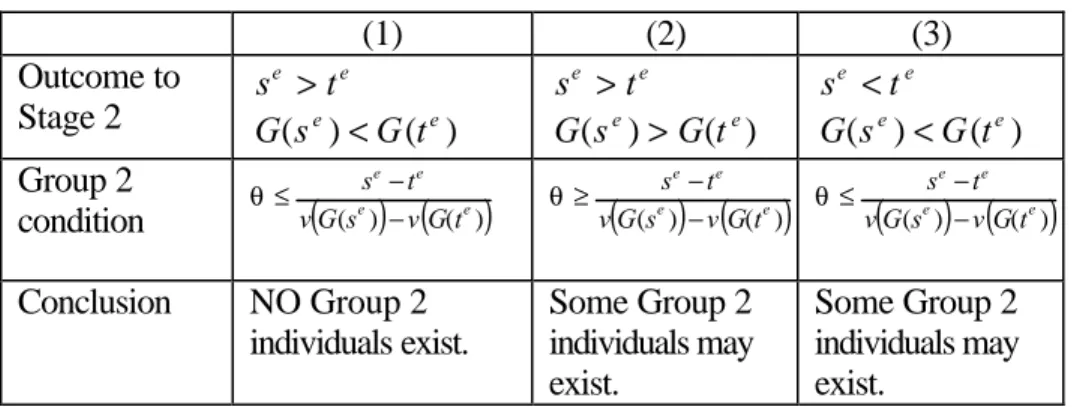
middle types when taxes provide more of the public good. Table 1 summarizes the

characteristics of Group 2 individuals depending on the outcome to Stage 2 of the voting process.

Table 1. Group 2 conditions and characteristics

(1) (2) (3) Outcome to Stage 2 e e _t s > ) ( ) (se G te G < e e _t s > ) ( ) (se G te G > e e _t s < ) ( ) (se G te G < Group 2 condition

(

( e)

) ( )

(e) e e t G v s G v t s − − ≤ θ

₍

_{) ( )}

) ( ) ( e e e e t G v s G v t s − − ≥ θ

₍

_{) ( )}

) ( ) ( e e e e t G v s G v t s − − ≤ θ Conclusion NO Group 2 individuals exist. Some Group 2 individuals may exist. Some Group 2 individuals may exist.

An equilibrium policy in Stage 1 is the policy that receives at least 50 percent of the votes. The proportion of individuals voting for fees is a coalition of Group 1 and Group 2 individuals. If the coalition of Group 1 individuals (non-subscribers who prefer paying

nothing under fees to paying a tax _te_{) and Group 2 individuals (subscribers under the fee}

who prefer the fee _se _{over the tax t}e

) exceeds 50 percent of individuals, then fee-based

provision is the equilibrium policy under majority-rule voting. Otherwise, tax-based

provision is the chosen policy. To shed more light on the sizes of groups 1 and 2, we now

Before we proceed, it is interesting to note that the coalition of individuals preferring fees to taxes can include individuals with a variety of different preferences depending on the outcome to Stage 2 of the game. When taxes provide more of the public good, we may have low and middle types preferring fees, with high types preferring taxes. However, when fees provide more of the good we can have low and high types preferring fees, with middle types preferring taxes, an ‘ends against the middle’ result similar to Epple and Romano (1996).

4. Numerical Results

In this section we solve a numerical example to show that an equilibrium under fee-based provision does exist.4 The numerical approach allows us to examine how variations in the

distribution of individual preferences affect the equilibrium policy choice. Solving the model numerically requires specifying functional forms for v(G) and F(θ), and assuming specific parameter values. The function that is used for v(G) throughout is

AG G G v + = 1 ) ( (19)

where A≥0. For A=0, we have v(G)=G. For A>0, v(G) is strictly concave, with the degree of concavity increasing as A rises. To allow for skewed preferences while at the same time maintaining a fairly simple distribution function, we use a ‘stepwise uniform’ distribution function for preferences where

θ θ γ θ γ θ θ γ θ θ γ θ θ θ γ θ θ ≤ < + ∀ + − + + = + ≤ ≤ ∀ + = ) 2 ( ) 1 ( 2 ) 2 ( 2 1 ) ( ) 2 ( 0 2 ) 2 ( ) ( F F (20)

with −1≤γ <∞. This distribution function was formed by taking a uniform distribution

between θ and θ, setting θ to zero, and defining the median preferences to be

) 2

( γ

θ

+ . This

functional form is chosen because it allows us to examine the effect of skewed preferences by changing only the parameter γ. 5

While facilitating the numerical calculations, the use of this distribution function also has intuitive appeal. For γ =0 we have a simple uniform distribution of types between 0 and θ with

median preferences of 2 θ

. For γ >0, preferences become right-skewed (i.e. the distribution of preferences becomes more dense on the low end). The individual with the median preferences has a type that approaches zero as γ approaches infinity. Graphically, the distribution of preferences with positive γ has the right-skewed shape of Figure 2.

Figure 2. A right-skewed distribution of preferences

) (θ f θ γ 2 ) 2 ( + ) 1 ( 2 ) 2 ( γ θ γ + + 0 ) 2 ( γ θ + θ θ 5

Numerical examples with other functional forms were investigated. However, alternative functional forms greatly increased the complexity of the calculations without generating any real additional insight.

However, left-skewed preferences can be analyzed by setting γ between 0 and -1. The median consumer has a type that approaches θ as γ approaches negative one. The distribution of preferences becomes more dense on the high end when γ is negative.

Table 2 presents the equilibrium values of θm, te =t(θm), and G(te) for specific parameter values of A, θ, and γ. The solutions are generated using A=0.25, θ=100, and letting γ vary from -0.6 (indicating left-skewed preferences) to 18 (indicating significantly right-skewed preferences). For γ =0, preferences are simply uniformly distributed and are symmetric and unskewed.

Table 2. Tax-based provision - Equilibrium values for _θm_,

) ( m

e _t

t = θ , and G(te) under

alternative parameterizations of the model.

Skewness Left Unskewed Right Right Right Parameter Values (1) γ=-0.6 (2) γ=0 (3) γ=2 (4) γ=8 (5) γ=18 m θ 71.4286 50 25 10 5 e t 29.8062 24.2843 16 8.6491 4.9443 ) (te G 29.8062 24.2843 16 8.6491 4.9443

The results shown in Table 2 indicate that, as expected, the equilibrium tax and public good levels fall as the median individual type falls (i.e. as γ increases). Note that it does not matter for the equilibrium tax how individuals above or below the median preference individual are distributed.

using the same parameter values as in the tax case.6 We derived these values by using the

properties established in Proposition 2 in the appendix and verifying that condition (A3) in the appendix holds for all fees below the smallest fee satisfying (10).7 This was the case for each of

the scenarios examined in our numerical solutions, implying that an equilibrium does indeed exist for each of the scenarios.8

Table 3. Fee-based provision - Equilibrium values for _θm_, ) (se

θ , θˆ(se), se, and G(se)

under alternative parameterizations of the model.

Skewness Left Unskewed Right Right Right Parameter Values (1) γ=-0.6 (2) γ=0 (3) γ=2 (4) γ=8 (5) γ=18 m θ 71.4286 50 25 10 5 ) (se θ 73.1424 53.6730 33.7508 35.9884 48.5217 ) ( ˆ e s θ 8.5689 7.3460 5.8339 5.7752 4.5812 e s 30.0204 25.0670 18.8072 17.4768 10.9432 ) (se G 28.2191 23.2248 16.6132 12.4305 5.9299

Several important results shown in Table 3 are worth emphasizing. First, the equilibrium fee in each case is a fee most preferred by an individual who has preferences above the median. For

6

Note that the sufficient condition G′′(s)<0 is satisfied in each case, implying single-peaked preferences. That is, G(s) is strictly concave.

7 _{Condition (A3) was verified numerically by first determining the appropriate expressions for} θ~_, θˆ_(s′_{), and} )

( ˆ _s

θ . The right-hand-side of (A3) was then subtracted from the left, and it was verified that the resulting expression remained positive for all fees below the smallest fee that satisfies (10). This was true for all of the parameterizations used here.

8

Note that θˆ(s) is increasing and convex for the lowest θˆ solution in each case (there are two θˆ, G solutions to (8) and (9). See appendix.) However, the function is relatively flat for the range of fees below the smallest fee that satisfies (10). These properties of the marginal consumer function can be seen by plotting θˆ for the parameter values that we used.

example, when θm =71.43, the equilibrium fee is 30.02 and is most preferred by an individual with type θ=73.14. When θm =5, the equilibrium fee is 10.94 and is most preferred by an individual with type θ= 48.52. Second, the relative distance between the median preference individual and the individual who most prefers the equilibrium fee increases as the distribution of preferences becomes more right-skewed.

Having found the outcomes for the tax and fee in Stage 2, the equilibrium policy choice can now be solved for. Note that a comparison of the public good levels (G(te)and G(se)in Tables 2 and 3, respectively), shows that provision of the public good is lower under fees in the left-skewed and uniform scenarios, but exceeds that under taxes in each of the three right-skewed scenarios. For example, when θm =50 (the uniform distribution case), G(se)=23.22 is lower than G(te)=24.28. But when θm =10 (a right-skewed distribution), G(te) is only 8.65 while

) (se

G is 12.43. This result is particularly important for determining the coalition of individuals that prefers fees to taxes in the policy choice stage.

Table 4 uses the conditions described in Section 2 regarding Group 1 and Group 2 individuals to calculate the proportion of individuals preferring fee-based provision to tax-based provision. Uniform and left-skewed distributions of preferences generate very little support for fee-based provision. For left-skewed preferences

(

γ =−0.6

)

, non-subscribers with type θ≤8.45 prefer fees and, therefore, belong to Group 1. There are 5.92% of individuals in that group. For uniformly distributed preferences

(

γ =0

)

, non-subscribers with type θ≤7.07 prefer fees and, therefore, belong to Group 1. Group 1 contains 7.07% of all individuals in that case. Because the tax provides more of the public good than the fee at a lower individual cost in both the

left-belonging to Group 1 increases as preferences move from left-skewed to uniform, but remains much less than a majority. Therefore, the equilibrium policy choice is a tax.

Table 4. Equilibrium policy outcomes.

Skewness Left Unskewed Right Right Right Parameter Values (1) γ=-0.6 (2) γ=0 (3) γ=2 (4) γ=8 (5) γ=18 LOW t θ~ condition 45 . 8 ≤ θ θ≤7.07 θ≤5.00 θ≤3.16 θ≤2.23 % in Group 1 5.92 7.07 10.00 15.81 22.36 HIGH θ~ condition NA NA θ≥118.02 θ≥30.33 θ ≥33.46 % in Group 2 0.00 0.00 0.00 38.71 35.02 % Vote for fee 5.92 7.07 10.00 54.52 57.38 Equilibrium Policy

TAX TAX TAX FEE FEE

As preferences become more right-skewed, two things happen: (1) the percentage of Group 1 individuals increases, and (2) the ranking of provision levels of the public good under taxes and fees reverses. The equilibrium fee remains higher than the equilibrium tax, and, eventually, the higher fee actually provides more of the public good than the tax. Although the fee provides more public good than the tax in the γ =2 scenario, the difference is too small to generate a positive number of Group 2 individuals. However, for γ =8 and γ =18, the higher provision under fees is sufficient to draw 38.71% and 35.02% of all individuals into Group 2, respectively. Combined with the 15.81% and 22.36% of Group 1 individuals, the coalition commands a majority, and fees are the equilibrium policy choice.

5. Welfare comparisons

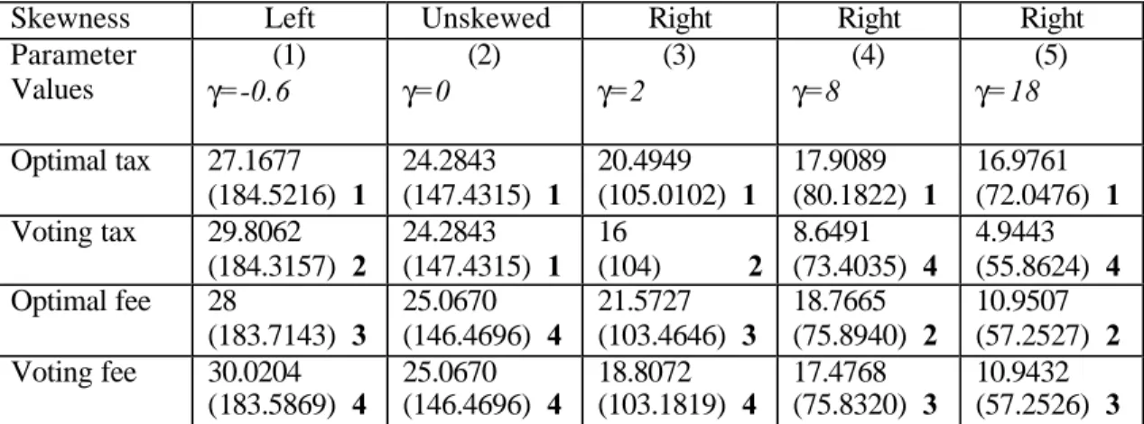
In this section we compare overall welfare under the equilibrium tax and fee for each of the five numerical cases. We also calculate the optimal (first-best) tax and optimal fee, according to a social planner’s problem, and their respective welfare levels, to include in the comparisons. We are particularly interested in ranking welfare under the four outcomes (optimal tax, optimal fee, voting tax, voting fee). Table 5 presents the numerical solutions to these outcomes for each of the five preference distributions. At this point we are ignoring Stage 1 of the previous analysis. That is, we are simply comparing welfare under the four plausible outcomes.

Table 5. Welfare comparisons.

Skewness Left Unskewed Right Right Right Parameter Values (1) γ=-0.6 (2) γ=0 (3) γ=2 (4) γ=8 (5) γ=18 Optimal tax 27.1677 (184.5216) 1 24.2843 (147.4315) 1 20.4949 (105.0102) 1 17.9089 (80.1822) 1 16.9761 (72.0476) 1 Voting tax 29.8062 (184.3157) 2 24.2843 (147.4315) 1 16 (104) 2 8.6491 (73.4035) 4 4.9443 (55.8624) 4 Optimal fee 28 (183.7143) 3 25.0670 (146.4696) 4 21.5727 (103.4646) 3 18.7665 (75.8940) 2 10.9507 (57.2527) 2 Voting fee 30.0204 (183.5869) 4 25.0670 (146.4696) 4 18.8072 (103.1819) 4 17.4768 (75.8320) 3 10.9432 (57.2526) 3

The optimal tax and fee are the tax or fee that maximizes utilitarian social welfare as given by the integral of the consumer utility function from θ to θ. The number in parentheses below each tax or fee is the level of social welfare provided at that tax or fee minus the endowment level. This number represents the total surplus welfare (beyond the endowment level) generated by that

case. For example, the bold number “1” in the optimal tax entry for case one indicates that the optimal tax provides the highest level of social welfare of the four different policies.

Several of the results shown in Table 5 are important. First, consistent with the results in Fraser (1996), the optimal tax provides the highest level of social welfare in all four cases. More importantly, however, are the relative welfare rankings of the remaining three policies. In the scenario with the most left-skewed preferences, the equilibrium voting tax provides the next highest level of social welfare, followed by the optimal fee and voting fee, in that order. In the second case with a simple uniform (unskewed) distribution of preferences, the optimal and voting taxes are identical and, therefore, provide identical levels of social welfare. Similarly, the optimal and voting fees are identical, but provide a level of social welfare below that of the two tax regimes.

The three skewed cases provide the most interesting results. In the least right-skewed case the rankings again are optimal tax, voting tax, optimal fee, voting fee, in that order. However, for cases four and five when the right-skewness is more extreme, the voting tax falls from second-best to fourth-best. In both cases, welfare under the voting fee exceeds that of the voting tax. Furthermore, as demonstrated in Section 4, a voting majority is also likely to prefer a fee to a tax in both cases.

6. Conclusions

Previous analyses of alternative methods of providing excludable public goods focus either on social welfare maximization or on profit maximization. Potential consumers are confronted with a tax or fee level that is determined by some means other than a democratic political process. However, when the public good in question is being provided by the state or some other form of representative government, it becomes necessary to consider the mechanisms

and forces that are likely to impact how and at what level the good is provided. These are, namely, the political process and the preferences of individual voters in the population. To the extent that majority-rule voting provides a reasonable approximation of the decision-making process for many goods that are publicly provided, the results from our model have important implications for a wide-range of goods from recreation to education.

The model demonstrates that, under majority-rule voting, the distribution of preferences for a public good is critical both in determining the level of provision under tax and fee alternatives, and in determining the policy preferred by the majority of individuals. Although the individual with the median preferences determines the equilibrium tax, an individual with preferences stronger than the median generally determines the equilibrium fee, when one exists. When preferences are distributed uniformly or are left-skewed, the majority of individuals prefers tax-based provision. Uniform and left-skewed distributions of preferences are also consistent with higher public good provision and higher social welfare under taxes. However, when preferences are right-skewed, the majority may prefer fee-based provision. Furthermore, the level of provision of the public good, as well as social welfare, may actually be higher under fees than under taxes in the latter case.

We made several assumptions that should be reconsidered in future research. For example, we assumed that individuals differ in preferences, but have identical incomes. Introducing heterogeneous incomes does not matter in the present model because utility is linear in m, and hence the size of the endowment does not affect individual preferences over the level of a tax or fee. An alternative formulation of the model would be to assume a different utility function and have heterogeneous endowments or income. Individual tax contributions could then

It is also worth emphasizing that the model assumes no externalities from the public good; non-subscribers are perfectly excluded and receive no utility from the public good. Clearly, many public goods have both excludable and non-excludable characteristics. For example, Yellowstone National Park is valued by park visitors because of the variety of camping, hiking, and sight-seeing opportunities they can enjoy. However, the park is arguably valued by many non-visitors for its mere ‘existence’. For the present purposes, we define the public good in question more narrowly; we include only those aspects of the good that benefit subscribers. Another important extension would be to allow for congestion externalities. In this case we suspect that the fee regime becomes even more attractive because the fee serves an important function to limit congestion.

Appendix

In this section we present the details and proofs of the results contained in Section 2.2, which characterizes the equilibrium fee under majority-rule voting.

Multiple Solutions

Multiple values for θˆ and G (equations (8) and (9)) may be possible for the same fee because of the interdependence between the marginal consumer type and the level of G that is provided. We pick the solution involving the lowest value for θˆ (i.e. the equilibrium that has the greatest number of subscribers) which corresponds to the highest public good provision. The greater the number of subscribers at a given fee, the higher the utility received by all existing subscribers because more public good is provided at the same cost to the individual. Also, the additional subscribers have higher utility because they previously had utility equal to m0, but by revealed preference, must have higher utility than m0, if they choose to subscribe. The utility of remaining non-subscribers is unchanged when additional individuals choose to subscribe.

Single-Peakedness of Preferences

In order to examine the existence and characteristics of an equilibrium fee, we first characterize the ordering of most preferred fees by individuals of different types and then identify a set of fees that would defeat any marginally larger or smaller fee in a pairwise vote. These fees serve as focal points for identifying an overall equilibrium fee, if one exists, and are referred to as local candidates. Finally, we characterize an overall equilibrium fee thereafter. An

the function s(θ) to denote the most preferred fee of an individual with type θ. We now establish a preliminary result.

Proposition 1: If G(s) is not too convex, then preferences over fees are single-peaked and )

(θ

s is non-decreasing in θ.

Proof: If an interior solution s∈(0,m₀)for an individual’s maximization problem exists, it is

characterized by

(

( )

)

( ) 0.

1+ ′ ′ =

− θv G s G s (A1)

The second order condition θ[v′

(

G(s)

)

G′′(s)+v′′

(

G(s)

)(

G′(s)

)

2]<0 is satisfied if

(

( )

)(

( )

)

/ '( ( )) )

(s v G s G s 2 v G s

G′′ <− ′′ ′ , that is, G(s)is not too convex. The interior solution applies if v'(0)G'(0)>1/θ and v'(m₀)G'(m₀)<1/θ. When v'(0)G'(0)<1/θ, the optimal fee is 0, and

if v'(m₀)G'(m₀) >1/θ, the optimal fee is m₀. In these boundary cases the most preferred fee is

constant in θ. For interior optimal fees, most preferred fees are strictly increasing in θ. To see this, differentiating (A1) shows that ds(θ)/dθ>0 if G(s) fulfills the convexity condition. Strict concavity of the maximization problem implies that preferences are single-peaked. Q.E.D.

Proposition 1 is an important property to keep the model tractable. Note that the assumption on G(s) is sufficient but not necessary to induce concavity of the induced preferences, which in turn is sufficient but not necessary for single-peakedness. It is difficult to state in terms of fundamentals what makes G(s) not too convex. The condition is useful

nevertheless for our computational analysis where it is shown to hold. For the following theoretical analysis we assume that G(s) satisfies the desired property.

Individuals with relatively strong preferences for the public good prefer to have higher fees imposed than individuals with relatively weak preferences. We can invert the function s(θ) and find for a given fee s the individual type who most prefers this fee. Denote this correspondence of most preferred fees to types as θ(s), which for an interior solution to the

problem above yields

(

( )

)

( ) 1 ) ( s G s G v s ′ ′ = θ .9

Necessary Conditions for Existence

We now wish to characterize the equilibrium fee. An equilibrium fee se under majority-rule voting is the fee that defeats any alternative fee sa ≠ sein a pairwise vote. When considering two fees, _s 1

and _s2

, an individual of type θ votes for the fee that yields higher utility. This means, an individual that would opt out at _s1

, but not at _s2

, must have higher utility under _s2 , and therefore, votes for _s2

. An individual who would opt out at both fees has utility of m₀ under

both fees, and is, therefore, indifferent between s 1 and s2. In such cases we assume that the individual abstains from voting.10

9

Note that θ(s)will technically be a function only if s(θ) is strictly increasing in θ for all θ. If a range of s

Proposition 2: Assume that s(θ)<s(θ) and more than half of the population prefers a fee

strictly between 0 and m0.

(a) A necessary condition for an equilibrium fee s is that s solves

(

( )

)

(

( )

)

( )

ˆ( )

1−F θ s = Fθ s −Fθ s , (A2)

where θ(s) is the individual who most prefers s, and θˆ(s) is the marginal consumer type

at s.

(b) There exists at least one fee for which (A2) holds.

(c) If an equilibrium fee exists, the equilibrium fee is the smallest of all fees that fulfill (A2).

Proof: (a) In condition (A2), the term 1−F

(

θ(s )

)

is the proportion of subscribers with type greater than θ(s)who prefer a higher fee, while F

(

θ(s)

)

−F

( )

θˆ(s) is the proportion of subscribers with type less than θ(s)who prefer a smaller fee. Suppose condition (A2) does not hold in a majority voting equilibrium. Then there exists a fee in the neighborhood of s which would win in a pairwise vote against s. If 1−F

(

θ(s)

)

<F

(

θ(s)

)

−F

( )

θˆ(s) , then a slightly smaller fee than s wins. A slightly higher fee wins in a pairwise vote if the inequality is reversed.

(b) Proposition 1 established that s(θ) is a continuous function. We assumed also that F(θ) is continuous. Begin by considering the most preferred fee of the lowest type individual s(θ). No individuals prefer a lower fee than s(θ), while by assumption a majority of individuals prefer a strictly higher fee. Therefore, s(θ)would lose to a slightly higher fee in a pairwise vote.

However, at the most preferred fee of the highest type individual s(θ), a majority of people would prefer a slightly lower fee, while no subscriber prefers a higher fee. Therefore, s(θ)would lose to a slightly smaller fee in a pairwise vote. By the Intermediate Value Theorem, there must exist at least one fee for which the proportion of individuals preferring a slightly higher fee exactly equals the proportion of individuals preferring a slightly lower fee.

(c) Suppose that _s1

and _s2

solve equation (9) and _s1 <_s2

. This implies by Proposition 1 that the individual types who prefer _s1

and _s2

satisfy θ(_s1)<θ(_s2)

. In addition, we know then that )) ( ( )) ( ( _s1 _{F s}2

F θ < θ . This, together with the fact that both fees solve (A2), implies )). ( ˆ ( )) ( ( )) ( ( 1 )) ( ( 1 )) ( ˆ ( )) ( ( s2 F s2 F s2 F s1 F s1 F s1 F θ − θ = − θ < − θ = θ − θ

Notice that this requires _F(θˆ(_s1))≤_F(θˆ(_s2))

, and hence implies also that θˆ(_s1)≤θˆ(_s2)

. It can now be shown that s1 wins against s2. Suppose that θˆ(s2)<θ(s1). All individuals with type

between θˆ(_s1)

and θ(_s1)

vote for _s1

. In addition, some individuals of a type slightly higher than )

(s1

θ vote for s1 as well. Let θ~ denote the individual who is just indifferent between s1 and

2

s . It must be the case that θ(_s1)<θ~<θ(_s2)

, and hence _F(θ~)> _F(θ(_s1))

. The fee _s1

wins a majority if F(θ~)−F(θˆ(s1))>1−F(θ~). This is the case because

) ~ ( 1 )) ( ( 1 )) ( ˆ ( )) ( ( )) ( ˆ ( ) ~ (θ _Fθ _s1 _F θ _s1 _F θ _s1 _F θ _s1 _F θ F − > − = − > − .

Alternatively, suppose that θˆ(s2)>θ(s1). For s1 to win a majority it is sufficient to

show that _F(θˆ(_s2))−_F(θˆ(_s1))>1−_F(θˆ(_s2)).

The intuition for part (c) is that an overall equilibrium fee must first be a local candidate that satisfies (A2), otherwise it would lose to a slightly larger or smaller fee in a pairwise vote. Moreover, only the smallest of the local candidate fees can be an overall equilibrium because a smaller local candidate will defeat a larger local candidate in a pairwise vote. This is because the smaller local candidate fee gets the vote from all subscribers below the individual who most prefers the smaller fee, and the smaller fee picks up some additional votes from a subset of individuals with only slightly higher θ types. In fact, if the non-convexity assumption of Lemma 1 holds throughout, as we assume it does, then the smallest local candidate will defeat any larger proposed fee in a pairwise vote. This is because preferences will be single-peaked, implying the marginal consumer will necessarily be non-decreasing in s, and the smallest local candidate will simply gain votes against any larger opponent by the same argument as above.

The identity of the decisive voter

Proposition 2 provides a necessary condition for an equilibrium fee to exist. However, the result does not rule out the possibility that a much smaller fee would beat in a pairwise comparison the smallest of all fees that satisfy (A2). Hence, a majority voting equilibrium may fail to exist. A sufficient condition for the candidate fee s to beat any other smaller fee s′ is

{

(ˆ( )), (ˆ( ))

}

min ) ~ ( ) ~ ( 1−F θ >F θ − F θ s′ F θ s (A3)

where θ~ is the individual who is indifferent between s and s′. It is easy to show that the sufficient condition is satisfied if θˆ(s′)>θˆ(s). However, this case is not likely to hold as we show later in numerical simulations. When θˆ(s′)<θˆ(s), it is difficult to prove that (A3) holds for all possible distributions F(θ). We therefore proceed under the assumption that the sufficient

condition is indeed satisfied. Generally speaking, this is the case if the function θˆ(s) is relatively flat because then the alternative fee s′ picks up few voters at the lower end and hence loses against s. Our numerical simulations show that this is the case.

This leads directly to the following result:

Proposition 3: If all individuals subscribe at the most preferred fee by the individual with median preference, then the equilibrium fee is the one preferred by the median person. Otherwise the equilibrium fee, when one exists, is higher than the one preferred by the median person.

Proof: If all individuals subscribe at s(θm), then s(θm)is the lowest local candidate, and no alternative lower fee can be introduced which defeats s(θm)because there are no additional individuals to subscribe. In that case, s(θm)satisfies all of the equilibrium conditions, and we have se = s(θm). However, if a positive number of individuals opt out at s(θm), then that fee cannot be an equilibrium fee under majority-rule voting. In that case, 50 percent of individuals prefer a slightly higher fee, while less than 50 percent prefer a lower fee because some individuals opt out and are indifferent. Q.E.D.

References

Black, Duncan, 1958, The Theory of Committees and Elections, Cambridge University Press.

Brito, Dagobert L., and William H. Oakland, 1980, On the monopolistic provision of excludable public goods, American Economic Review 70, 691-704.

Buchanan, J. M., 1965, An economic theory of clubs, Economica 33, 1-14.

Burns, M.E, and C. Walsh, 1981, Market provision of price-excludable public goods: A general analysis, Journal of Political Economy 89, 166-191.

Downs, Anthony, 1957, An Economic Theory of Democracy, New York: Harper and Row. Epple, Dennis, and Richard E. Romano, 1996, Ends against the middle: Determining

public service provision when there are private alternatives, Journal of Public Economics 62, 297-325.

Fraser, C. D., 1996, On the provision of excludable public goods, Journal of Public Economics 60, 111-130.

Fretwell, Holly Lippke, 1999, Paying to Play: The Fee Demonstration Program, PERC Policy Series PS-17, December.

Helsley, Robert W., and William C. Strange, 1998, Private Government, Journal of Public Economics 69, 281-304.

Helsley, Robert W., and William C. Strange, 1991, Exclusion and the theory of clubs, Canadian Journal of Economics 4, 889-899.

Laux-Mieselbach, W., 1988, Impossibility of exclusion and characteristics of public goods, Journal of Public Economics 36, 127-137.

Oakland, W. H., 1972, Congestion, public goods, and welfare, Journal of Public Economics 1, 339-357.

Silva, Emilson C.D., and Charles M. Kahn, 1993, Exclusion and Moral Hazard: The case of identical demand, Journal of Public Economics 52, 216-235.

U.S. Senate, 1999, Committee on Energy and Natural Resources, Recreation Fee Demonstration Program, Hearings...106th Congress, 1st Session.