A Survey of GPU-Based Large-Scale Volume Visualization

A Survey of GPU-Based

Large-Scale Volume Visualization

The Harvard community has made this

article openly available. Please share how

this access benefits you. Your story matters

Citation

Beyer, Johanna, Markus Hadwiger, and Hanspeter Pfister. 2014.

A Survey of GPU-Based Large-Scale Volume Visualization. In the

Proceedings of The Eurographics Conference on Visualization

(Eurovis 2014), Swansea, Wales, June 9-13, 2014.

Citable link

http://nrs.harvard.edu/urn-3:HUL.InstRepos:21150340

Terms of Use

This article was downloaded from Harvard University’s DASH

repository, and is made available under the terms and conditions

applicable to Open Access Policy Articles, as set forth at

http://

nrs.harvard.edu/urn-3:HUL.InstRepos:dash.current.terms-of-use#OAP

Eurographics Conference on Visualization (EuroVis) (2014) R. Borgo, R. Maciejewski, and I. Viola (Editors)

A Survey of GPU-Based Large-Scale Volume Visualization

Johanna Beyer1, Markus Hadwiger2, Hanspeter Pfister1

1_{Harvard University, USA}

2_{King Abdullah University of Science and Technology, Saudi Arabia}

Abstract

This survey gives an overview of the current state of the art in GPU techniques for interactive large-scale volume visualization. Modern techniques in this field have brought about a sea change in how interactive visualization and analysis of giga-, tera-, and petabytes of volume data can be enabled on GPUs. In addition to combining the parallel processing power of GPUs with out-of-core methods and data streaming, a major enabler for interactivity is making both the computational and the visualization effort proportional to the amount and resolution of data that is actually visible on screen, i.e., “sensitive” algorithms and system designs. This leads to recent output-sensitive approaches that are “ray-guided,” “visualization-driven,” or “display-aware.” In this survey, we focus on these characteristics and propose a new categorization of GPU-based large-scale volume visualization techniques based on the notions of actual output-resolutionvisibilityand the current working setof volume bricks—the current subset of data that is minimally required to produce an output image of the desired display resolution. For our purposes here, we view parallel (distributed) visualization using clusters as an orthogonal set of techniques that we do not discuss in detail but that can be used in conjunction with what we discuss in this survey.

Categories and Subject Descriptors (according to ACM CCS): I.3.6 [Computer Graphics]: Methodology and Techniques—I.3.3 [Computer Graphics]: Picture/Image Generation—Display algorithms

1. Introduction

Visualizing volumetric data plays a crucial role in scien-tific visualization and is an important tool in many domain sciences such as medicine, biology and the life sciences, physics, and engineering. The developments in GPU tech-nology over the last two decades, and the resulting vast par-allel processing power, have enabled compute-intensive op-erations such as ray-casting of large volumes at interactive rates. However, in order to deal with the ever-increasing res-olution and size of today’s volume data, it is crucial to use highly scalable visualization algorithms, data structures, and architectures in order to circumvent the restrictions imposed by the limited amount of on-board GPU memory.

Recent advances in high-resolution image and volume ac-quisition, as well as computational advances in simulation, have led to an explosion of the amount of data that must be visualized and analyzed. For example, high-throughput elec-tron microscopy can produce volumes of scanned brain tis-sue at a rate above 10-40 megapixels per second [BLK∗11], with a pixel resolution of 3-5 nm. Such an acquisition pro-cess produces almost a terabyte of raw data per day. For the next couple of years it is predicted that new multi-beam electron microscopes will further increase the data ac-quisition rate by two orders of magnitude [Hel13,ML13].

This trend of acquiring and computing more and more data at a rapidly increasing pace (“Big Data”) will continue in the future [BCH12]. This naturally poses significant chal-lenges to interactive visualization and analysis. For exam-ple, many established algorithms and frameworks for vol-ume visualization do not scale well beyond a few giga-bytes, and this problem cannot easily be solved by simply adding more computing power or disk space. These chal-lenges require research on novel techniques for data visual-ization, processing, storage, and I/O that scale to extreme-scale data [MWY∗09,AAM∗11,BCH12].

Today’s GPUs are very powerful parallel processors that enable performing compute-intensive operations such as ray-casting at interactive rates. However, the memory sizes available to GPUs are not increasing at the same rate as the amount of raw data. In recent years, several GPU-based methods have been developed that employ out-of-core meth-ods and data streaming to enable the interactive visualiza-tion of giga-, tera-, and petabytes of volume data. The cru-cial property that enables these methods to scale to extreme-scale data is theiroutput-sensitivity, i.e., that they make both the computational and the visualization effort proportional to the amount of data that is actually visible on screen (i.e., the output), instead of being proportional to the full amount

of input data. In graphics, the focus of most early work on output-sensitive algorithms was visibility determination of geometry (e.g., [SO92,GKM93,ZMHH97]).

An early work in output-sensitive visualization on GPUs was dealing with 3D line integral convolution (LIC) volumes of flow fields [FW08]. In the context of large-scale volume visualization, output-sensitive approaches are often referred to as beingray-guided(e.g., [CNLE09,Eng11,FSK13]) or

visualization-driven(e.g., [HBJP12,BHAA∗13]). These are the two terms that we will use most in this survey.

We use the termvisualization-drivenin a more general and inclusive way, i.e., these methods are not necessarily bound to ray-casting (which is implied by “ray-guided”), and they can encompass all computation and processing of data in addition to rendering. In principle, the visual out-put can “drive” the entire visualization pipeline—including on-demand processing of data—all the way back to the raw data acquisition stage [HBJP12,BHAA∗13]. This would then yield a fullyvisualization-driven pipeline. However, to a large extent these terms can be used interchangeably.

Another set of output-sensitive techniques are display-awaremulti-resolution approaches (e.g., [JST∗10,JJY∗11, HSB∗12]). The main focus of these techniques is usually output-sensitive computation (such as image processing) rather than visualization, although they are also guided by the actual display resolution and therefore the visual output. Ray-guided and visualization-driven visualization tech-niques are clearly inspired by earlier approaches for oc-clusion culling (e.g., [ZMHH97,LMK03]) and level of de-tail (e.g., [LHJ99,WWH∗00]). However, they have a much stronger emphasis on leveraging actual output-resolution visibilityfor data management, caching, and streaming—in addition to the traditional goals of faster rendering and anti-aliasing. Very importantly, actual visibility is determined on-the-fly during visualization, directly on the GPU.

1.1. Survey Scope

This survey focuses on major scalability properties of ume visualization techniques, reviews earlier GPU vol-ume renderers, and then discusses modern ray-guided and visualization-driven approaches and how they relate to and extend the standard visualization pipeline (see Figure 1). Large-scale GPU volume rendering can be seen as being in the intersection of volume visualization and high perfor-mance computing. General introductions to these two topics are given in books on real-time volume graphics [EHK∗06] and high performance visualization [BCH12], respectively.

We mostly focus on techniques for stand-alone worksta-tions with standard graphics hardware. We see the other core topics of high performance visualization (i.e., paral-lel rendering on CPU/GPU clusters, distributed visualization frameworks, and remote rendering) as an orthogonal set of

techniques that can be used in combination with modern ray-guided, visualization-driven, and display-aware techniques as discussed here. Therefore, for more details on parallel vi-sualization we refer the reader to previous surveys in this area [Wit98,BSS00,ZSJ∗05]. Nonetheless, where parallel or distributed rendering methods do directly relate to our course of discussion we have added them to our exposition.

We focus on volume rendering of regular grids and mostly review methods for scalar data and a single time step. How-ever, the principles of the discussed scalable methods are general enough that they also apply to variate, multi-modal, or time series data. For a more in-depth discussion of the visualization and visual analysis of multi-faceted sci-entific data we refer the reader to a recent comprehensive survey [KH13]. Other related recent surveys can be found on the topics of compression for GPU-based volume render-ing [RGG∗13], and massive model visualization [KMS∗06].

1.2. Survey Structure

This survey gives an overview of the current state of the art in large-scale GPU volume visualization. Starting from the standard visualization pipeline in Section2, we discuss required modifications and extensions to this pipeline to achieve scalability with respect to data size (see Figure1).

We continue by examining general scalability issues and how they relate to and are used in volume visualization (Section3). This includes scalable data structures as well as data layout and compression for efficient data access on disk (Section3.1). Next, we discuss different approaches for partitioning data and/or work to achieve scalable per-formance, from potentially in-core domain decomposition to out-of-core approaches (Section3.2), before describing dif-ferent ways to reduce the computational load, focusing on on-demand processing, streaming, and in-situ visualization approaches (Section3.3).

Section4discusses recent advances in large-scale volume rendering in depth, starting with a review of traditional GPU volume rendering techniques and their limitations.

We focus on the characteristics of recent ray-guided, visualization-driven, and display-aware techniques (Sec-tion4.1). To reflect and emphasize these recent advances, we propose a new categorization of GPU-based large-scale volume visualization techniques (Table3) based on the no-tion of the active working set—the current subset of data that is minimally required to produce an output image of the desired display resolution.

We discuss methods for determining the working set, i.e., culling (Section4.2), GPU data structures for storing the working set (Section4.3), and the actual ray-casting meth-ods for rendering the working set (Section4.4).

Finally, we review the major challenges and current limi-tations and give an outlook on future trends and open prob-lems in large-scale GPU volume visualization (Section5).

Visualization

Processing

Data

Image

Data (Pre-)

Processing Filtering Mapping Rendering Data Representation On-Demand Processing Acceleration Metadata Ray-Guided Rendering

Scalability

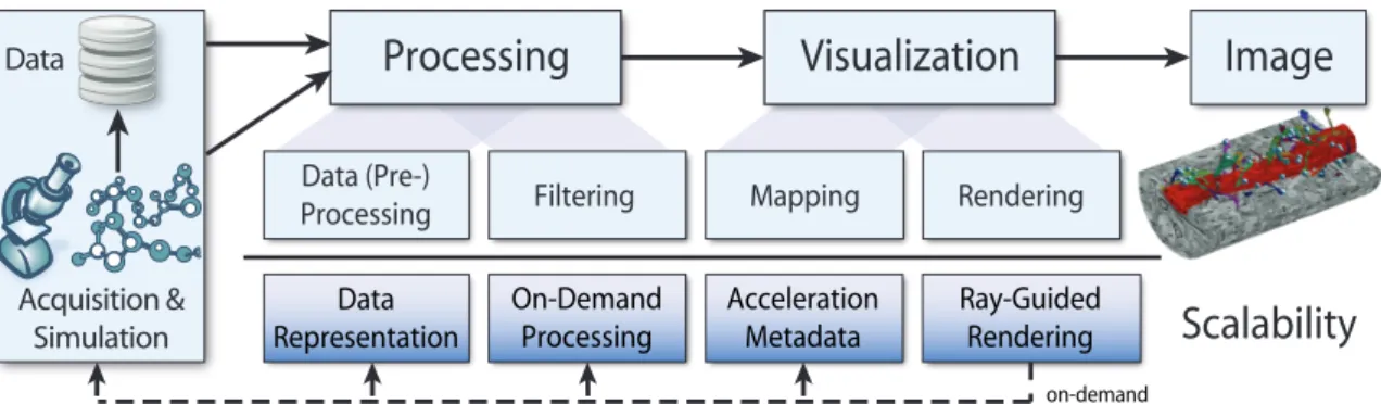
Figure 1:The visualization pipeline for large-scale visualization.Data are generated on the left (either through acquisi-tion/measurement or through computation/simulation) and then pass through a sequence of stages that culminate in the desired output image. The related high-level aspects with respect to scalability of interactive volume rendering are highlighted in the bottom row. Aray-guidedorvisualization-drivenapproach can drive earlier pipeline stages so that only what is required by (visible in) the output image is actually loaded or computed. In a fully visualization-driven pipeline, this approach can be carried through from rendering (determining visibility) on the right all the way back to data acquisition/simulation on the left.

2. Fundamentals

We first introduce a few basic concepts and give a conceptual overview of the visualization pipeline with respect to large-scale volume visualization.

2.1. Basic Concepts

Large-scale visualization. In the context of this survey, large-scale visualization deals with volume data that do not completely fit into memory. In our case, the most important memory type is GPU on-board memory, but scalability must be achieved throughout the entire memory hierarchy. Most importantly, large-scale volume data cannot be handled di-rectly by volume visualization techniques that assume that the entire volume is resident in memory in one piece.

Bethel et al. [BCH12] (Chapter 2) define large data based on three criteria: They are too big to be processed: (1) in their entirety, (2) all at one time, and (3) exceed the avail-able memory. Scalavail-able visualization methods and architec-tures tackle either one or a combination of these criteria.

Scalability.In contrast to parallel/distributed visualization, where a major focus is onstrongvs.weakscaling [CPA∗10], we define scalability in terms ofoutput-sensitivity[SO92]. Our focus are algorithms, approaches, and architectures that scale to large data by making the computation and visual-ization effort proportional to both thevisibledata on screen and the actualscreen resolution. If the required size of the

working setof data is independent of the original data size, we say that an approach isscalablein this sense.

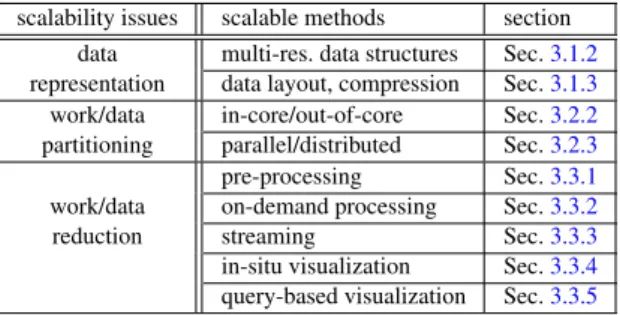
Scalability issues. Based on the notion of large data, the main scalability issues for volume rendering deal with ques-tions on how to represent data, how to split up the work and/or data to make it more tractable, and how to reduce the amount of work and/or data that has to be handled. Table1

lists these main issues and the general methods that are used in large-scale visualization to handle them.

Acceleration techniques vs. data size.A common source of confusion when discussing techniques for scalable volume rendering is the real goal of a specific optimization tech-nique. While many of the techniques discussed in this sur-vey were originally proposed as performance optimizations, they can also be adapted to handle large data sizes. A well-known example of this are octrees. While octrees are often used in geometry rendering to speed up view frustum culling (via hierarchical/recursive culling), an important goal of us-ing octrees in volume renderus-ing is to enable adaptive level of detail [WWH∗00], in addition to enabling empty space skipping. This “dual” purpose of many scalable data struc-tures and algorithms is an important issue to keep in mind.

Output-sensitive algorithms.The original focus of output-sensitive algorithms [SO92] was making theirrunning time

dependent on the size of theoutput instead of the size of theinput. While this scalability in terms of running time is of course also important in our context, for the work that we discuss here, it is even more important to consider the dependence on output “data size” vs. input data size, using the concept of theworking setas described above.

Ray-guided and visualization-driven architectures. In line with the concepts outlined above, these types of archi-tectures focus most of all on data management (processing, streaming, caching) rather than only on rendering. While ray-casting intrinsically could be called “ray-guided,” this by itself is not very meaningful. The difference to stan-dard ray-casting first arises from how and which data are streamed into GPU memory, i.e.,ray-guided streamingof volume data [CNLE09]. Again considering the working set, a ray-guided approach determines the working set of volume bricksviaray-casting. That is, the working set comprises the bricks that are intersected during ray traversal. It is common

scalability issues scalable methods section data multi-res. data structures Sec.3.1.2

representation data layout, compression Sec.3.1.3

work/data in-core/out-of-core Sec.3.2.2

partitioning parallel/distributed Sec.3.2.3

pre-processing Sec.3.3.1

work/data on-demand processing Sec.3.3.2

reduction streaming Sec.3.3.3

in-situ visualization Sec.3.3.4

query-based visualization Sec.3.3.5

Table 1:Scalability considerations in large-scale volume visualization.Scalability issues, the corresponding methods to tackle them, and where they are covered in this survey.

to determine the desired level of detail, i.e., the (locally) re-quired volume resolution, during ray-casting as well.

In this way, data streaming is guided by theactual vis-ibility of data in the output image. This is in contrast to the approximate/conservative visibility obtained by all com-mon occlusion culling approaches. As described in the intro-duction,visualization-drivenarchitectures generalize these concepts further to ultimately drive the entire visualization pipeline by actual on-screen visibility [HBJP12,BHAA∗13].

2.2. Large-Scale Visualization Pipeline

A common abstraction used by visualization frameworks is thevisualization pipeline[Mor13]. In essence, the visualiza-tion pipeline is a data flow network where nodes or mod-ules are connected in a directed graph that depicts the data flow throughout the system (see Figure1). After data ac-quisition or generation through computation/simulation, the first stage usually consists of some kind of data processing, which can include many sub-tasks from datapre-processing

(e.g., computing a multi-resolution representation) to filter-ing. The second half of the pipeline comprises the actual vi-sualization, includingvisualization mappingandrendering.

For large-scale rendering, all the stages in this pipeline have to be scalable (i.e., in our context: output-sensitive), or they will become the bottleneck for the entire application. The bottom part of Figure1shows the main techniques em-ployed by state-of-the-art visualization-driven pipelines to achieve this scalability: Multi-resolution and compact data representations, on-demand processing based on the visible subset currently in view, acceleration data (e.g., for faster ray traversal or empty space skipping), and ray-guided rendering with dynamic ray traversal.

Table1gives an overview of the most important scalabil-ity aspects of large-scale visualization frameworks that we will use later. Actual scalability also depends on how dy-namically and accurately the working set is determined, how volumes are represented, and how ray traversal is performed. We discuss individual visualization methods in Section4.

3. Basic Scalability Techniques

This section introduces the main considerations and tech-niques for designing scalable volume visualization archi-tectures in general terms. In real-world applications, these strategies for handling and rendering large data often have to be combined to achieve interactive performance and high-quality images.

For future ultra-scale visualization and exa-scale comput-ing [ALN∗08,SBH∗08,MWY∗09,AAM∗11,Mor12] it is es-sential that each step of the visualization pipeline is fully scalable.

3.1. Data Representation and Storage

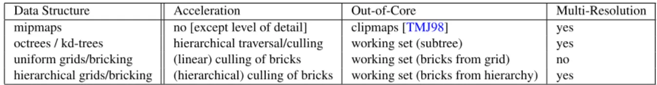
Efficient data representation is a key requirement for scal-able volume rendering. Scalscal-able data structures should be compact in memory (and disk storage), while still being ef-ficient to use and modify. Table2lists common related data structures and their scalability aspects. Additional GPU rep-resentations of these data structures, as they are used for ren-dering, are discussed in Section4.4.

3.1.1. Bricking

Bricking is an object space decomposition method that sub-divides the volume into smaller, box-shaped sub-volumes, orbricks. Commonly, all bricks have the same size in vox-els (e.g., 323or 2563voxels per brick). Volumes that are not a multiple of the basic brick size are padded accordingly. Bricking facilitates out-of-core approaches because individ-ual bricks can be loaded and rendered as required, without having to load/stream the volume in its entirety.

Bricked data usually require special handling of brick boundaries. Operations where neighboring voxels are re-quired (e.g., GPU texture filtering, gradients) usually return incorrect results at brick boundaries, because the neighbor-ing voxels are not readily available. The correct voxels can be fetched from the neighboring bricks [Lju06a], which is costly. More commonly, so-calledghost voxels[ILC10] are employed, which are duplicated voxels at the brick bound-aries that enable straightforward, correct filtering. The use of ghost voxels is the standard approach in most bricked ray-casters [BHWB07,FK10]. Ghost voxels are usually stored with each brick on disk, but they can also be computed on-the-fly in a streaming fashion [ILC10].

The recent OpenGL extension for virtual texturing (GL_ARB_sparse_texture) includes hardware support for texture filtering across brick boundaries and thus allevi-ates the need for ghost voxels.

Choosing the optimal brick size depends on several crite-ria and has been studied in the literature [HBJP12,FSK13]. Small bricks support fine-grained culling, which results in smaller working sets. However, the ghost voxel overhead

Data Structure Acceleration Out-of-Core Multi-Resolution mipmaps no [except level of detail] clipmaps [TMJ98] yes

octrees / kd-trees hierarchical traversal/culling working set (subtree) yes uniform grids/bricking (linear) culling of bricks working set (bricks from grid) no hierarchical grids/bricking (hierarchical) culling of bricks working set (bricks from hierarchy) yes

Table 2:Scalable data structures for volume visualization.Our categorization is based on their support for acceleration (skipping, culling), out-of-core processing/rendering, and support for multi-resolution rendering (i.e., adaptive level of detail).

grows for smaller bricks, and the total number of bricks in-creases as well. The latter makes a multi-pass rendering ap-proach where each brick is rendered individually infeasible. Typically, traditional multi-pass out-of-core volume ren-derers use relatively large bricks (e.g., 1283or 2563) to re-duce the number of required render passes. In contrast, mod-ern single-pass ray-casters use smaller bricks (e.g., 323), or a hybrid approach where small bricks are used for render-ing and larger bricks are used for storage on disk [HBJP12, FSK13]. For 2D data acquisition modalities such as mi-croscopy, hybrid 2D/3D tiling/bricking strategies have also been employed successfully, for example via on-demand computation of 3D bricks from pre-computed 2D mipmap tiles during visualization [HBJP12,BHAA∗13].

3.1.2. Multi-Resolution Hierarchies

One of the main benefits of multi-resolution hierarchies for rendering large data is that they allow sampling the data from a resolution level that is adapted to the current screen reso-lution or desired level of detail. This reduces the amount of data to be accessed and also avoids aliasing artifacts due to undersampling.

Trees (octrees, kd-trees). Octrees [WWH∗00,Kno06] and kd-trees [FCS∗10] are very common 3D multi-resolution data structures for direct volume rendering. They allow efficient traversal and directly support hierarchical empty space skipping. Traditional tree-based volume renderers em-ploy a multi-pass rendering approach where one brick (one tree node) is rendered per rendering pass. Despite the hi-erarchical nature of these data structures, many early ap-proaches assume that the entire volume fits into mem-ory [LHJ99,WWH∗00,BNS01]. Modern GPU approaches support traversing octrees directly on the GPU [GMG08, CNLE09,CN09,RTW13], which is usually accomplished via standard traversal algorithms from the ray-tracing litera-ture [AW87,FS05,HSHH07,PGS∗07,HL09].

In recent years,sparse voxel octrees(SVOs) have gained a lot of attention in the graphics and gaming industry [LK10a, LK10b]. Several methods for rendering large and complex voxelized 3D models use SVO data structures for efficient rendering [GM05,R¨09,HN12,Mus13].

Mipmaps are a standard multi-resolution pyramid repre-sentation that is very common in texture mapping [Wil83].

Mipmaps are supported by virtually all GPU texture units. Clipmaps [TMJ98] are virtualized mipmaps of arbitrary size. They assume a moving window (like in terrain rendering) that looks at a small sub-rectangle of the data and use a toroidal updating scheme for texels in the current view.

Hierarchical grids with bricking.Another type of multi-resolution pyramids are hierarchical grids where each reso-lution level of the data is bricked individually. These grids have become a powerful alternative to octrees in recent ray-guided volume visualization approaches [HBJP12,FSK13]. The basic approach can be viewed as bricking each level of a mipmap individually. However, more flexible systems do not use hardware mipmaps and therefore allow varying down-sampling ratios between resolution levels [HBJP12]—e.g., for anisotropic data—which is not possible with mipmaps.

Since there is no tree structure in such a grid type, no tree traversal is necessary during rendering. Rather, the entire grid hierarchy is viewed as a huge virtual address space (avirtual texture), where any voxel corresponding to data of any resolution can be accessed directly via ad-dress translationfromvirtualtophysicaladdresses [vW09, BHL∗11,OVS12]. On GPUs, this address translation can be performed via GPU “page tables,” which is also possi-ble in amulti-levelway for extremely large data [HBJP12] (see Section 4.4.1). As in the case of bricking with uni-form grids, interpolation between bricks has to be handled carefully. Especially transitions between different resolu-tion levels can introduce visual artifacts, and several meth-ods have been introduced that deal with correct interpola-tion [Lju06a,Lju06b,BHMF08].

Wavelet representations.Muraki [Mur93] first introduced wavelet transforms for volume rendering. Subsequent meth-ods such as Guthe et al. [GGSe∗02,GS04] compute a hier-archical wavelet representation in a pre-process and decom-press the bricks required for rendering

Other representations.Younesy et al. [YMC06] have pro-posed improving the visual quality of multi-resolution vol-ume rendering by approximating the voxel data distribution by its mean and variance at each level of detail. The recently introduced sparse pdf maps represent the data distribu-tion more accurately, allowing for the accurate, anti-aliased evaluation of non-linear image operators on gigapixel im-ages [HSB∗12]. The corresponding data structure is very similar to standard mipmaps in terms of storage and access.

3.1.3. Data Layout and Compression

Data layout.To efficiently access data on disk, data lay-out and access are often optimized. In general, reading small bits of data at randomly scattered positions is a lot more inefficient than reading larger chunks in a continu-ous layout. Therefore, locality-preserving data access pat-terns such as space filling curves, e.g., Morton (z-) or-der [Mor66] are often used in time-critical visualization frameworks [SSJ∗11]. A nice feature of the Morton/z-order curve is that by adjusting the sampling stride along the curve, samples can be restricted to certain resolution levels. Pas-cucci and Frank [PF02] describe a system for progressive data access that streams in missing data points for higher resolutions. With the most recent solid state drives (SSDs), however, trade-offs might be different in practice [FSK13].

Data compression.Another major related field is data com-pression, for disk storage as well as for the later stages of the visualization pipeline. We refer to the recent compre-hensive survey by Rodriguez et al. [RGG∗13] for an in-depth discussion of the literature on volume compression andcompression-domainvolume rendering.

3.2. Work/Data Partitioning

A crucial technique for handling large data is topartitionor

decomposedata into smaller parts (e.g., sub-volumes). This is essentially adivide and conquer strategy, i.e., breaking down the problem into several sub-problems until they be-come easier to solve. Partitioning the data and/or work can alleviate memory constraints, complexity, and allow paral-lelization of the computational task. In the context of visual-ization, this includes ideas like domain decomposition (i.e., object-space and image-space decompositions), but also en-tails parallel and distributed visualization approaches.

3.2.1. Domain Decompositions

Object-space (data domain) decomposition is usu-ally done by using bricking with or without a multi-resolution representation, as described in Sections 3.1.1 and 3.1.2, respectively. Object-space decompositions are view-independent and facilitate scalability with respect to data size by storing and handling data subsets separately.

Image-space (image domain) decompositionsubdivides the output image plane (the viewport) and renders the result-ing image tiles independently. A basic example of this ap-proach is ray-casting (which is animage-order approach), where conceptually each pixel is processed independently. In practice, several rays (e.g., a rectangular image tile) are processed together in some sense. For example, rendering each image tile in a single rendering pass, or assigning each tile to a different rendering node. Another example is ren-dering on a large display wall, where each individual screen is assigned to a different rendering node.

3.2.2. Out-Of-Core Techniques

Unless when dealing with data that is small enough to fit into memory (“in core”) in its entirety, one always has to parti-tion the data and/or computaparti-tion in a way that makes it pos-sible to process subsets of the data independently. This en-ables out-of-core processing and can be applied at all stages of the visualization pipeline [SCC∗02,KMS∗06]. Different levels of out-of-core processing exist, depending on where the computation is performed and where the data is residing (either on the GPU, CPU, hard-disk, or network storage).

Out-of-core methods include algorithms that focus on accessing [PF02] and prefetching [CKS03] data, creating on-the-fly ghost data for bricked representa-tions [ILC10], and methods for computing multi-resolution hierarchies [HBJP12] or other processing tasks such as segmentation [FK05], PDE solvers [SSJ∗11], image reg-istration and alignment [JST∗10], or level set computa-tion [LKHW04].

Silva et al. [SCC∗02] give a comprehensive overview of out-of-core methods for visualization and graphics.

3.2.3. Parallel and Distributed Rendering

High-performance visualization often depends on dis-tributed approaches that split the rendering of a data set between several nodes of a cluster. The difference can be defined such thatparallel visualization approaches run on a single large parallel platform, whereas distributed ap-proaches run on a heterogeneous network of computers. Molnar et al. [MCE∗94] propose a classification of paral-lel renderers intosort-first,sort-middle, andsort-last. In the context of large data volume rendering,sort-lastapproaches are very popular. In this context, this term refers to brick-ing the data and makbrick-ing each node responsible for renderbrick-ing one or several bricks before final image compositing. In con-trast, sort-first approaches subdivide the viewport and assign render nodes to individual image tiles. Neumann [Neu94] examines the communication costs for different parallel vol-ume rendering algorithms.

Conceptually, all or any parts of the visualization pipeline can be run as a distributed or parallel system. Recent de-velopments in this field are promising trends towards exa-scale visualization. However, covering the plethora of dis-tributed and parallel volume visualization approaches is out of scope of this survey. The interested reader is referred to [Wit98,BSS00,ZSJ∗05] and [BCH12] (Chapter 3) for in-depth surveys on this topic.

3.3. Work/Data Reduction

Reducing the amount of data that has to be processed or ren-dered is a major strategy for dealing with large data. Tech-niques for data reduction cover a broad scope, ranging from multi-resolution data representations and sub-sampling to

more advanced filtering and abstraction techniques. A dis-tinction has to be made between data reduction for storage (e.g., compression) that tries to reduce disk or in-memory size, and data reduction for rendering. The latter encom-passes visualization-driven and display-aware rendering ap-proaches as well as more general methods such as on-demand processing and query-based visualization.

3.3.1. Pre-Processing

Running computationally expensive or time-consuming computations as a pre-process to compute acceleration meta-data or pre-cache meta-data can often dramatically reduce the computation costs during rendering. Typical examples in-clude pre-computing a multi-resolution hierarchy of the data that is used to reduce the amount of data needed for ren-dering. On the other hand, processing data interactively dur-ing renderdur-ing can reduce the required disk space [BCH12] (Chapter 9), and enables on-demand processing, which in turn can reduce the amount of data that needs processing.

3.3.2. On-Demand Processing

On-demand strategies determine at run time which parts of the data need to be processed, thereby eliminating pre-processing times and limiting the amount of data that needs to be handled. For example, ray-guided and visualization-driven volume rendering systems only request volume bricks to be loaded that are necessary for rendering the current view [CNLE09,HBJP12,FSK13]. Data that is not visible is never rendered, processed, or even loaded from disk.

Other examples for on-the-fly processing for volume vi-sualization target interactive filtering and segmentation. For example, Jeong et al. [JBH∗09] have presented a system where they perform on-the-fly noise removal and edge en-hancement during volume rendering only for the currently visible part of the volume. Additionally, they perform an interactive active-ribbon segmentation on a dynamically se-lected subset of the data.

3.3.3. Streaming

In streaming approaches, data are processed as they become available (i.e., are streamed in). Streaming techniques are closely related to on-demand processing. However, where the latter usually consists of apull model(i.e., data is re-quested by a process), streaming can be a pull or apush model(i.e., new data is pushed to the next processing step).

Streaming also facilitates circumventing the need for the entire data set to be available before the visualization starts and allows rendering of incomplete data [SCC∗02]. Had-wiger et al. [HBJP12] have described a system for streaming extreme-scale electron microscopy data for interactive visu-alization. This system has later been extended to include on-the-fly registration and multi-volume visualization of seg-mented data [BHAA∗13]. Further streaming-based

visual-ization frameworks include the dataflow visualvisual-ization sys-tem presented by Vo et al. [VOS∗10], which is built on top of VTK and implements a push and pull model.

3.3.4. In-Situ Visualization

Traditionally, visualization is performed after all data have been generated—either by measurement or simulation—and have been written to disk. In-situ visualization, on the other hand, runs simultaneously to the on-going simulation (e.g., on the same supercomputer or cluster:in situ—in place), with the aim of reducing the amount of data that needs to be transferred and stored on disk [BCH12] (Chapter 9).

To avoid slowing down the primary simulation,in-transit

visualization accesses only “staging” nodes of a simulation cluster. The goal of these nodes is to hide the latency of disk storage from the main simulation by handling data buffering and I/O [MOM∗11].

In-situ and in-transit visualization have been identi-fied as being crucial for future extreme-scale comput-ing [MWY∗09,AAM∗11,KAL∗11,Mor12]. Furthermore, when the visualization process is tightly coupled or inte-grated into the simulation, these approaches can be lever-aged for computational steering, where simulation pa-rameters are changed based on the visualization [PJ95, TTRU∗06]. Yu et al. [YWG∗10] present a complete case study of in-situ visualization for a petascale combustion sim-ulation. Tikhonova et al. [TYC∗11] take a different approach by generating a compact intermediate representation of large volume data that enables fast approximate rendering for pre-view and in-situ setups.

3.3.5. Query-based Visualization

Query-driven visualization uses selection as the main means to reducing the amount of data that needs to be pro-cessed [BCH12] (Chapter 7). Prominent techniques are dy-namic queries [AWS92], high-dimensional brushing and linking [MW95], and interactive visual queries [DKR97]. Shneiderman [Shn94] gives an introduction to dynamic queries for visual analysis and information seeking.

The DEX framework [SSWB05] focuses on query-driven scientific visualization of large data sets using bitmap index-ing to quickly query data. Recently, approaches for query-based volume visualization have been introduced in the con-text of neuroscience [BvG∗09,BAaK∗13], with the goal to analyze the connectivity between individual neurons in elec-tron microscopy volumes. The ConnectomeExplorer frame-work [BAaK∗13] implements visual queries on top of a large-scale, visualization-driven system.

4. Scalable Volume Rendering Techniques

In this section we categorize and discuss the individual liter-ature in GPU-based large-scale volume rendering. We start

working set

determination full volume

basic culling ray-guided / (global, view frustum) visualization-driven volume data

representation

linear (non-bricked) single-resolution grid octree octree volume storage [HSSB05] [BHWB07] [LHJ99] [WWH∗00] [GMG08]‡ [CN93] [CCF94] [WE98] [GGSe∗02] [GS04] [CNLE09] [Eng11]

[RSEB∗00] [HBH03] grid with octree [PHKH04] [HFK05] [RTW13] [LMK03]†[RGW∗03] per brick kd-tree

[KW03] [SSKE05] [RV06] [FK10] multi-resolution grid

[BG05] [MHS08] [HBJP12] [BAaK∗13] [KGB∗09]†[MRH10] multi-resolution grid [FSK13] [Lju06a] [BHMF08] [JBH∗09] rendering (ray traversal)

texture slicing CPU octree traversal (multi-pass) GPU octree traversal [CN93] [CCF94] [WE98] [LHJ99] [WWH∗00] [GGSe∗02] (single-pass)

[RSEB∗00] [HBH03] [GS04] [PHKH04] [HFK05] [RV06] [GMG08]‡ [LMK03]† CPU kd-tree traversal (multi-pass) [CNLE09] [Eng11]

[FK10] [RTW13]

non-bricked ray-casting

(multi-pass) bricked/virtual texture multi-level virtual texture [RGW∗03] [KW03] ray-casting (single-pass) ray-casting (single-pass) (single-pass) [HSSB05] [Lju06a] [BHWB07] [HBJP12] [BAaK∗13] [SSKE05] [BG05] [MHS08] [BHMF08] [JBH∗09] [FSK13]

[KGB∗09]†[MRH10]

scalability low medium high

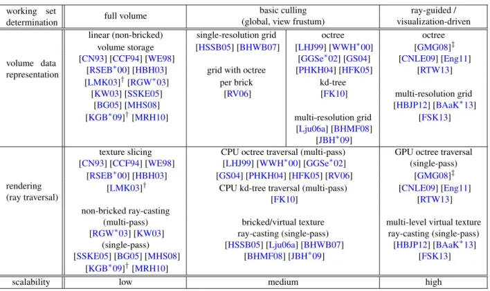
Table 3:Categorization of GPU-based volume visualization techniquesbased on the type ofworking set determination mech-anism and the resultingscalabilityin terms of data size, as well as according to the volume data representation employed, and the actual rendering technique (type of ray traversal; except in the case of texture slicing).†[LMK03,KGB∗09] perform culling for empty space skipping, but store the entire volume in linear (non-bricked) form.‡[GMG08] is not fully ray-guided, but utilizes interleaved occlusion queries with similar goals (see the text).

with an overview of “traditional” GPU-based volume ren-dering techniques, before we go into details on “modern” ray-guided and visualization-driven techniques.

Categorization (Table 3).We categorize GPU-based vol-ume rendering approaches with respect to their scalability properties by using the central notion of theworking set— the subset of volume bricks that is required for rendering a given view. Using the concept of working set, our catego-rization distinguishes different approaches according to: 1. How the working set is determined.

2. How the working set is stored (represented) on the GPU. 3. How the working set is used (accessed) during rendering. We elaborate on these categories below in (1) Section4.2, (2) Section4.3, and (3) Section4.4.

We also categorize the resultingscalability(low, medium, high), where only “high” scalability means full output-sensitivity and thus independence of the input volume size.

The properties of different volume rendering approaches—and the resulting scalability—vary greatly between what we refer to as “traditional” approaches (cor-responding to “low” and “medium” scalability in Table3),

and “modern” ray-guided approaches (corresponding to “high” scalability in Table3).

A key feature of modern ray-guided and visualization-driven volume renderers is that they make full use of re-cent developments in GPU programmability. They usually include a read-back mechanism to update the current work-ing set, and traverse a multi-resolution hierarchy dynami-cally on the GPU. This flexibility was not possible on earlier GPUs and is crucial for determining an accurate working set.

4.1. GPU-Based Volume Rendering

GPUs have, over the last two decades, become very versa-tile and powerful parallel processors, succeeding the fixed-function pipelines of earlier graphics accelerators. Gen-eral purpose computing on GPUs (GPGPU)—now also called GPU Compute—leverages GPUs for non-graphics re-lated and compute-intensive computations [OLG∗07], such as simulations or general linear algebra problems. In-creased programmability has been made possible by APIs like the OpenGL Shading Language (GLSL) [Ros06] and CUDA [NVI13].

Figure 2:Rendering a multi-gigabyte CT data set (as used in [Eng11]) at different resolution levels using a ray-guided rendering approach. Data courtesy of Siemens Healthcare, Components and Vacuum Technology, Imaging Solutions. Data was reconstructed by the Siemens OEM reconstruction API CERA TXR (Theoretically Exact Reconstruction).

However, GPU on-board memory sizes are much more limited than those of CPUs. Therefore, large-scale volume rendering on GPUs requires careful algorithm design, mem-ory management, and the use of out-of-core approaches.

4.1.1. Traditional GPU-Based Volume Rendering

Before discussing current state-of-the-art ray-guided volume renderers, we review traditional GPU volume rendering ap-proaches. We start with 2D and 3D texture slicing methods, before continuing with GPU ray-casting. This will give us the necessary context for categorizing and differentiating be-tween the more traditional and the more modern approaches.

Texture slicing. The earliest GPU volume rendering ap-proaches were based on texture mapping [Hec86] using 2D and 3D texture slicing [CN93,CCF94]. Westermann and Ertl [WE98] extended this approach to support arbitrary clip-ping geometries and shaded iso-surface rendering. For cor-rect tri-linear interpolation between slices, Rezk-Salama et al. [RSEB∗00] made use of multi-texturing. Hadwiger et al. [HBH03] described how to efficiently render segmented volumes on GPUs and how to perform two-level volume rendering on GPUs, where each labeled object can be ren-dered with a different render mode and transfer function. This approach was later extended to ray-casting of multi-ple segmented volumes [BHWB07]. Engel et al. [ESE00] were among the first to investigate remote visualization us-ing hardware-accelerated renderus-ing.

Texture slicing and parallel volume rendering. Texture slicing has been used in many distributed and parallel volume rendering systems [MHE01,CMC∗06,MWMS07, EPMS09,FCS∗10]. Magallon et al. [MHE01] used sort-last rendering on a cluster, where each cluster node renders one

volume brick before doing parallel compositing for final im-age generation. For volume rendering on small to medium GPU clusters, Fogal et al. [FCS∗10] introduced a load-balanced sort-last renderer integrated into VisIt [CBB∗05], a parallel visualization and data analysis framework for large data sets. Moloney et al. [MWMS07] proposed a sort-first technique using eight GPUs, where the render costs per pixel are used for dynamic load balancing between nodes. They later extended their method to support early ray termination and volume shadowing [MAWM11]. Equalizer [EPMS09] is a GPU-friendly parallel rendering framework that supports both sort-first and sort-last approaches.

Texture slicing today.In general, the advantage of texture slicing-based volume renderers is that they have minimum hardware requirements. 2D texture slicing, for example, can be implemented in WebGL [CSK∗11] and runs efficiently on mobile devices without 3D texture support. However, a disadvantage is that they often exhibit visual artifacts and less flexibility when compared to ray-casting methods.

Ray-casting. Röttger et al. [RGW∗03] and Krüger and Westermann [KW03] were among the first to perform ray-casting on GPUs, using a multi-pass approach. Ray-ray-casting is embarrassingly parallel and can be implemented on the GPU in a fragment shader or compute kernel, where each fragment or thread casts one ray through the volume. Ray-casting easily admits a wide variety of performance and quality enhancements such as empty space skipping and early ray termination. Hadwiger et al. [HSSB05] and Stegmaier et al. [SSKE05] were among the first to perform GPU ray-casting using a single-pass approach, taking advan-tage of dynamic looping and branching in then-recent GPUs. Proxy geometries for efficient empty space skipping can be based on bricks [HSSB05,SHN∗06], spheres [LCD09], or occlusion frustums [MRH08].

Müller et al. [MSE06] used GPU ray-casting in a sort-last parallel rendering system. With the introduction of CUDA as a higher-level GPU programming language, CUDA-based ray-casters were introduced [MHS08,KGB∗09,MRH10]. They make use of CUDA’s thread/block architecture, and possibly shared memory model.

Large data. For rendering large data, several multi-resolution octree rendering methods have been proposed, most of them based on texture-slicing [LHJ99,WWH∗00, GGSe∗02,GS04,PHKH04]. Hong et al. [HFK05] used a min-max octree structure for ray-casting the Visible Hu-man CT data set. To support volumes that are larger than GPU memory, bricked single-pass ray-casting can be used [HSSB05,BHWB07,JBH∗09]. These techniques access volume bricks stored in a large brick cache (or brick pool) texture, which is similar to adaptive texture maps [KE02]. However, the brick cache is usually managed dynamically to accommodate transfer function changes. Ljung et al. [Lju06a] used a multi-resolution bricking struc-ture and adaptive sampling in image- and object-space to

Figure 3:Per-sample LOD selectionas in [HBJP12]. Left: electron microscopy volume (90 GB). Middle and right: the LOD used for each sample is color-coded. Middle: discrete LOD for each sample (tri-linear interpolation). Right: frac-tional LOD for each sample, with interpolation between data of neighboring LODs (“quad-linear” interpolation).

render large data. Beyer et al. [BHMF08] proposed a tech-nique for correct interpolation between bricks of two differ-ent resolution levels.

A lot of research has focused on remote, parallel, or dis-tributed visualization for rendering large data, which we can-not all cover here. For example, Prohaska et al. [PHKH04] used an octree approach to remotely render large remote micro-CT scans, while Wang et al. [WGL∗05] proposed a wavelet-based time space partitioning tree for volume ren-dering of large time varying volumes but use a parallel CPU ray-caster on a PC cluster for rendering.

A different approach to dealing with large data was pro-posed by Turlington et al. [THM01], who introduced slid-ing thin slab (STS) visualization to limit the amount of data needed for any current view. Knoll et al. [KTW∗11] op-timized CPU ray-casting, achieving interactive rates using a bounding volume hierarchy (BVH) min/max acceleration structure and SIMD optimizations.

4.1.2. Ray-Guided Volume Rendering

Ray-guided and visualization-driven volume rendering ap-proaches incorporate a feedback loop between the ray-caster and the culling mechanism, where the ray-caster itself writes out accurate information on missing bricks and brick usage. Thus, this type of culling mechanism determines an accurate working set directly on the GPU.

This information about the working set is then used to load missing data, and to determine which bricks can be evicted from the GPU cache because they are no longer needed. Additionally, rays automatically determine the (lo-cally) required data resolution. This determination can be performed either on a per-sample basis [HBJP12] (see Fig-ure3), or on a per-brick basis [FSK13].

Gobbetti et al. [GMG08] were among the first to imple-ment a volume ray-caster with stackless GPU octree traver-sal. They used occlusion queries to determine, load, and pos-sibly refine visible nodes. This approach already has similar properties to later fully ray-guided approaches. However, it

is strictly speaking not fully ray-guided, because culling of octree nodes is performed on the CPU based on the occlu-sion query information obtained from the GPU.

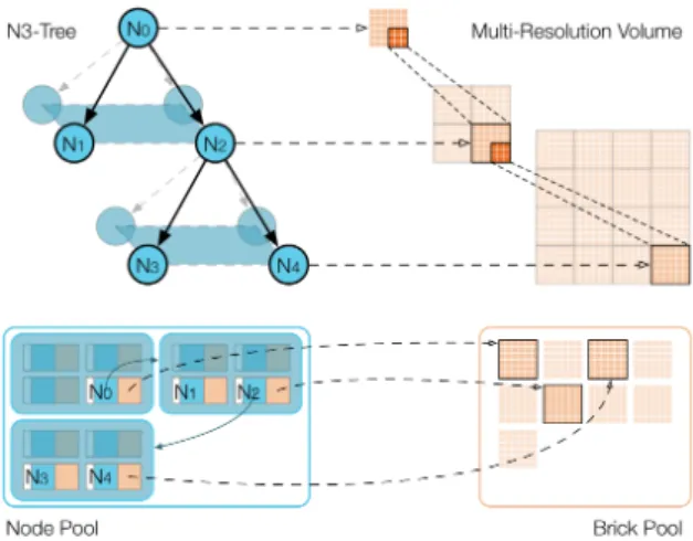
Crassin et al. [CN09] introduced the Gigavoxels system for GPU-based octree volume rendering with ray-guided streamingof volume data. Their system can also make use of anN3 tree, as an alternative to an octree (which would be anN3tree withN=2). The tree is traversed at run time using the kd-restart algorithm [FS05] and active tree nodes stored in anode pool. Actual voxel data are fetched from bricks stored in abrick pool. Each node stores a pointer to its child nodes in the node pool, and a pointer to the associated texture brick in the brick pool (see Figure4). The focus of the Gigavoxels system is volume rendering for entertainment applications and as such it does not support dynamic transfer function changes [CNSE10]. The more recent CERA-TVR system [Eng11] targets scientific visualization applications and supports fully dynamic updates according to the transfer function in real time. It also uses the kd-restart algorithm for octree traversal. Reichl et al. [RTW13] also employ a similar ray-guided approach, but target large smooth particle hydro-dynamics (SPH) simulations.

A different category of ray-guided volume renderers uses hierarchical grids with bricking, which are accessed via multi-level page tables instead of a tree structure. Hadwiger et al. [HBJP12] proposed such a multi-resolution virtual memory scheme based on a multi-level page table hierarchy (see Figure5). This approach scales to petavoxel data and can also efficiently handle highly anisotropic data, which is very common in high-resolution electron microscopy vol-umes. They also compare their approach for volume traver-sal to standard octree travertraver-sal in terms of travertraver-sal complex-ity and cache access behavior, and illustrate the advantages of multi-level paging in terms of scaling to very large data.

Fogal et al. [FSK13] have performed an in-depth analysis of several aspects of ray-guided volume rendering.

4.2. Working Set Determination

Performing culling to determine the current working set of bricks is crucial for ray-casting large data at interactive frame rates. Originally, culling was introduced for geome-try rendering, where view frustum and occlusion culling are used to limit the number of primitives that have to be ren-dered. Ideally, alloccludedgeometry should be culled before rendering.

4.2.1. View Frustum Culling

Removing primitives or volume bricks outside the current view frustum is the most basic form of culling. The first step of GPU ray-casting consists of computing the ray start points and end points (often via rasterization), which already pre-vents sampling the volume in areas that are outside the view

Figure 4:The Gigavoxels systemuses an N3tree structure with node and brick pools that store the set of active nodes and bricks, respectively.

frustum. However, in order to prevent volume bricks out-side the frustum from being downloaded to the GPU, the individual bricks have to be culled against the view frustum. Naturally, if a brick lies completely outside the current view frustum, it is not needed in GPU memory. Culling a view frustum against a bounding box, a bounding volume hier-archy, or a tree can be done very efficiently and has been studied extensively [AM00,AMHH08].

4.2.2. Global, Attribute-Based Culling

Another way to cull bricks in volume rendering is based on global properties like the current transfer function, iso value, or enabled segmented objects. Culling against the transfer function is usually done based on min/max computations for each brick [PSL∗98,HSSB05,SHN∗06]. The brick’s min/max values are compared against the transfer function to determine if the brick is invisible (i.e., only contains values that are completely transparent in the transfer function). In-visible bricks are then culled. The downside of this approach is that it needs to be updated whenever the transfer function changes and usually needs pre-computed min/max values for each brick that have to be available at runtime for all bricks. A similar approach can be used for culling bricks against an iso-surface [PSL∗98,HSSB05], or against enabled/disabled objects in segmented volume rendering [BHWB07].

4.2.3. Occlusion/Visibility Culling

Occlusion or visibility culling tries to cull primitives in-side the view frustum that are occluded by other primitives. While this is easier for opaque geometry, in (transparent) volume rendering this process is more involved and often requires a multi-pass rendering approach.

Greene et al. [GKM93] introduce hierarchical z-buffer visibility. They use two hierarchical data structures, an oc-tree in object space and a z-pyramid in image space to

quickly reject invisible primitives in a hierarchical man-ner. Zhang et al. [ZMHH97] propose hierarchical occlusion maps (HOMs), where a set of occluders is rendered into a low-resolution occlusion map that is hierarchically down-sampled and used to test primitives for occlusion before ren-dering them.

For volume visualization, Li et al. [LMK03] introduce occlusion clipping for texture-based volume rendering to skip rendering of occluded parts of the volume. Gao et al. [GHSK03] propose visibility culling in large-scale par-allel volume rendering based on pre-computing a plenop-tic opacity function per brick. Visibility culling based on temporal occlusion coherence has also been used for time-varying volume rendering [GSHK04]. The concept of oc-clusion culling has also been used in a parallel setting for sort-last rendering [MM10], by computing and propagating occlusion information across rendering nodes.

4.2.4. Ray-Guided Culling

Ray-guided culling approaches are different in the sense that they start with an empty working set. Only bricks that are actually visited during the ray-casting traversal step are re-quested and subsequently added to the working set of active bricks. Therefore, this approach implicitly culls all occluded bricks, as well as bricks outside the view frustum.

Gobbetti et al. [GMG08] use a mixture of traditional culling and ray-guided culling. They first perform culling on the CPU (using the transfer-function, iso value, and view frustum), but refine only those nodes of the octree that were marked as visible in the previous rendering pass. To deter-mine if a node is visible they use occlusion queries to check the bounding box of a node against the depth of the last vis-ited sample that was written out during ray-casting.

Crassin et al. [CN09] originally used multiple render tar-gets to report which bricks were visited by the ray-caster over the course of several frames, exploiting spatial and tem-poral coherence. The same information was constructed in a more efficient way using CUDA in a later implementa-tion [CNSE10].

Hadwiger et al. [HBJP12] divide the viewport into smaller tiles and use a GPU hash table per image tile to report a limited number of cache misses. Over the course of several frames, this ensures that all missing bricks are reported.

Fogal et al. [FSK13] use a similar approach built on lock-free hash tables.

4.3. Working Set Storage and Access

Efficient GPU data structures for storing the working set should be fast to access during ray traversal, and should also support efficient dynamic updates of the working set. Recent approaches usually store volume bricks (actual voxel data) in a singe large 3D cache texture (or brick pool).

Multi-Resolution Page Directory Virtual Page Tables Virtual Voxel Volumes resolution hierarchy l=2 323 _voxel brick 323 _page table entries single page directory entry single page table entry Page Table Cache Brick Cache Multi-Resolution Page Directory l=1 l=0 l=2 Virtual Volume Cache Miss Hash Table l=0 l=1

page table hier

ar

ch

y

virtualized

Ray-Casting

Virtual Memory Architecture

Figure 5:Multi-resolution, multi-level GPU page tables[HBJP12]. The virtual memory architecture comprises two orthogonal hierarchies: the resolution hierarchy, and the page table hierarchy. Ray-casting performs address translation based on the multi-resolution page directory (i.e., one page directory per volume resolution) and shared “mixed-resolution” cache textures.

If ray traversal needs to follow tree nodes (as in octree-based renderers), the working set of tree nodes must also be stored, e.g., in anode pool(e.g., [CNLE09,Eng11]).

If ray traversal is built on virtual to physical address trans-lation (as in page table-based renderers), the working set of page table entries must be stored, e.g., in apage table cache

(e.g., [BHL∗11,HBJP12]).

4.3.1. Texture Cache Management

Texture allocation.Early tree-based volume renderers often employed one texture per brick, rendering one after the other in visibility order using one rendering pass per brick/tree node [LHJ99,WWH∗00,GGSe∗02,GS04]. However, multi-pass approaches are usually less performant than single-multi-pass approaches and are also limited in the number of passes they can efficiently perform. To circumvent rendering bottlenecks due to many rendering passes, Hong et al. [HFK05] cluster bricks in layers (based on the manhattan distance) and render all bricks of the same layer at the same time.

To support single-pass rendering, bricking approaches and modern ray-guided renderers usually use a single large 3D cache texture (or brick pool) to store the working set [BHWB07,CN09,HBJP12], and often assume that the working set will fit into GPU memory.

When the working set does not fit into GPU memory, ei-ther the level of detail and thus the number of bricks in the working set can be reduced [HBJP12], or the renderer can switch to a multi-pass fall-back [Eng11,FSK13].

Texture updates.Whenever the working set changes, the cache textures have to be updated accordingly. Hadwiger et al. [HBJP12] compare texture update complexity between octree-based and multi-level page table approaches. Octree-based approaches usually have to do a large number of

up-dates of small texture elements, whereas hierarchical page tables tend to perform fewer but larger updates.

To avoid cache thrashing [HP11], different brick replace-ment strategies have been introduced. Most common is the LRU scheme which replaces the brick in the cache that was least recently used [GMG08,CN09,FSK13]. It is also com-mon to use a hybrid LRU/MRU scheme, where the LRU scheme is used unless the cache is too small for the cur-rent working set. In the latter case, the scheme is switched to MRU (most recently used) to reduce cache thrashing.

4.3.2. Virtual Texturing and Address Translation Page tables.Kraus and Ertl [KE02] were the first to intro-duce adaptive texture maps for GPUs, where an image or volume can be stored in a bricked fashion with adaptive res-olution and accessed via a look-up in a small index texture. This index texture can be seen as a page table [HP11].

Virtual texturing.Going further in this direction leads to virtual texturing [OVS12], also called Megatextures in game engines [vW09], and partially resident textures [BSH12]. A single, very large virtual texture is used for all data instead of allocating many small textures.

During rendering, virtual texture coordinates have to be translated to physical texture coordinates. Recently, hard-ware implementations of this scheme have become available with the OpenGLGL_ARB_sparse_textureextension. Unfortunately, current hardware limitations still limit the size of these textures to 16k pixels/voxels and do not allow for automatic page fault handling.

GPU-based page tables for virtual texturing are con-ceptually very similar to CPU virtual memory architec-tures [HP11]. For volume rendering, the virtual volume is decomposed into smaller bricks (i.e, pages), and a look-up

texture (i.e., page table) maps from virtual pages to physical pages. The earliest uses of virtual texturing and page tables in volume rendering [HSSB05] used a single page table tture. However, the basic concept of virtualization can be ex-tended in a “recursive” fashion, which leads to apage table hierarchy. Virtual texturing architectures using such multi-level page tables have been shown to scale to volume data of extreme scale [BHL∗11,HBJP12].

Hadwiger et al. [HBJP12] describe level, multi-resolution page tables as a (conceptually) orthogonal 2D structure (see Figure5, left). One dimension corresponds to the page table hierarchy, consisting of the page directory (the top-level page table) and several page tables below. The sec-ond dimension correspsec-onds to the different resolution lev-els of the data. Each resolution level conceptually has its own page table hierarchy. However, the actual cache tex-tures can be shared between all resolution levels. Multi-level page tables scale very well. For example, two levels have been shown to support volumes of up to several hundred ter-abytes, and three levels should in principle be sufficient even for exascale data [HBJP12] (in terms of “addressability”).

Octrees.To traverse an octree directly on the GPU, not only the volume brick data, but also a (partial) tree needs to be stored on the GPU. Gobbetti et al. [GMG08] use a spatial index structure to store the current subtree with neighbor in-formation. Each octree node stores pointers to its eight chil-dren and its six neighbors (via ropes [HBZ98]), and a pointer to the volume brick data. Crassin et al. [CN09,CNLE09] use anN3tree, whose current subtree is stored in a node pool and a brick pool, respectively. Each node stored in the node pool contains one pointer to itsN3children, and one pointer to the corresponding volume brick in the brick pool (see Figure4). Using a single child pointer is possible because the children are stored together in the node pool.

Hash tables.An alternative data structure to GPU page ta-bles are hash tata-bles, which have not yet received a lot of at-tention for large-scale volume rendering. However, Hastings et al. [HMG05] use spatial hashing to optimize collision de-tection in real-time simulations, and Nießner et al. [NZIS13] use voxel hashing for real-time 3D reconstruction.

4.4. Rendering (Ray Traversal)

In this section we will look into details of the actual ren-dering methods and how dynamic address translation is per-formed on the GPU.

Single-pass vs. multi-pass. In single-pass approaches the volume is traversed in front-to-back order in a single render-ing pass as compared to multi-pass approaches that require multiple rendering passes. As mentioned before, the first GPU volume rendering approaches [CN93,CCF94,WE98, RSEB∗00,HBH03], including the first octree-based ren-derers [LHJ99,WWH∗00,GGSe∗02,GS04,HFK05], were

all based on multi-pass rendering. With the introduc-tion of dynamic branching and looping on GPUs, single-pass approaches have been introduced to volume ray-casting [HSSB05,SSKE05].

Multi-pass approaches offer a higher flexibility, however, they also have a significant management overhead compared to single-pass rendering (i.e., context switching, final com-positing) and usually result in lower performance. Further-more, optimization techniques like early ray termination are not trivial in multi-pass rendering and create an additional overhead. Therefore, most state-of-the art ray-guided vol-ume renderers use single-pass rendering [CNLE09,Eng11, HBJP12]. A limitation of single-pass approaches, however, is the requirement for the entire working set to fit into the cache. One way to circumvent this requirement is to use single-pass rendering as long as the working sets fits into the cache, and to switch to multi-pass rendering when the working set gets too large [Eng11,FSK13].

Multi-resolution rendering.There are several motivations for multi-resolution rendering. Next to the obvious advan-tage of data reduction and rendering speed-ups, choosing a resolution that matches the current screen resolution reduces aliasing artifacts due to undersampling [Wil83].

A multi-resolution data structure requires level-of-detail (LOD) or scale selection [LB03] for rendering. Weiler et al. [WWH∗00] us a focus point oracle based on the dis-tance from the center of a brick to a user-defined focus point to select a brick’s LOD. Other methods to select a level of detail include estimating the screen-space er-ror [GS04], using a combined factor of data homogene-ity and importance [BNS01] or using the predicted visual significance of a brick [Lju06b]. A common method esti-mates the projected screen space size of the corresponding voxel/brick [CNLE09]. Whereas LOD selection is often per-formed on a per-brick basis, Hadwiger et al. [HBJP12] select the LOD on a per-sample basis for finer LOD granularity (see Figure3).

The most common data refinement strategy (e.g., when quickly zooming-in on the data) consists of a “greedy” ap-proach that iteratively loads the next higher-resolution of the brick until the desired resolution is reached [CNLE09]. A different approach, where the highest resolution is loaded di-rectly and intermediate resolutions are skipped was proposed in [HBJP12]. Most recently, Fogal et al. [FSK13] found that the “greedy” approach converges in the fewest number of frames in their ray-guided ray-caster.

4.4.1. Virtual Texturing and Address Translation

Address translation is performed during ray-casting, when stepping along a ray, to access the correct location of a sam-ple along the ray in the texture cache. When using multi-resolution data this implies that a GPU multi-multi-resolution data structure has to be traversed dynamically on the GPU.

Tree traversal.Traversal algorithms for efficiently navigat-ing and traversnavigat-ing trees, such as kd-trees or octrees have been well researched in the ray-tracing community. Ama-natides and Woo [AW87] were the first to introduce a fast regular grid traversal algorithm. Recently, stackless traver-sal methods such as kd-restart [FS05] have received a lot of attention [HSHH07,PGS∗07,HL09], as they are well-suited for GPU implementation.

The GPU octree traversal in Gobbetti et al. [GMG08] is based on previous work on rope trees [HBZ98,PGS∗07], whereas Gigavoxels [CNLE09,CNSE10] and similar sys-tems [Eng11,RTW13] base their octree traversal on the kd-restart algorithm [FS05].

Page table look-ups.In virtual texturing approaches [vW09, OVS12,HBJP12], each texture sample requires address translation from a virtual texture coordinate to a correspond-ing physical texture coordinate durcorrespond-ing rendercorrespond-ing. This trans-lation is done via small look-up texture(s), thepage table(s). In multi-level page tables, additional levels of page ta-bles are added [BHL∗11]. The top level is usually called the

page directory, in analogy to CPU virtual memory [HP11]. The right part of Figure5depicts address translation dur-ing ray-castdur-ing with a multi-resolution, multi-level page ta-ble. Hadwiger et al. [HBJP12] use this approach for render-ing extreme-scale electron microscopy data. Their approach starts with computing a LOD for the current sample, which is then used to look up the page directory corresponding to that resolution. Next, address translation traverses the page table hierarchy from the page directory through the page table lev-els below. Previous page directory and page table look-ups can be cached to exploit spatial coherence. Thus, the number of texture look-ups that is required in practice is very low.

Handling missing and empty bricks.In contrast to tradi-tional ray-casting approaches, where the working set is com-puted prior to rendering on the CPU, ray-guided volume ren-ders only build up the current working set during ray traver-sal. This implies that ray-guided volume renderers have to be able to deal with missing bricks in GPU memory, be-cause bricks are only requested and downloaded once they have been hit during ray-casting.

Whenever the ray-caster detects a missing brick (i.e., ei-ther a page table entry that is flagged asunmappedor a miss-ing octree node), a request for that missmiss-ing brick is written out. Crassin et al. [CN09] use multiple render targets to re-port missing nodes and then stop ray traversal. More recent approaches [CNSE10,HBJP12,FSK13] use OpenGL exten-sions such as GL_ARB_shader_image_load_store or CUDA, and often GPU hash tables, to report cache misses. Missing bricks can be either skipped, or substituted by a brick of lower resolution. After missing bricks are de-tected and reported, the CPU takes care of loading the miss-ing data, downloadmiss-ing it into GPU memory, and updatmiss-ing the corresponding GPU data structures.

Figure 6: Ray-guided volume rendering [FSK13] of the Mandelbulb data set. Colors indicate the amount of empty space skipping and sampling that needs to be performed (green: skipped empty brick, red: densely sampled brick, blue: densely sampled but quickly saturated). Image cour-tesy of Tom Fogal.

Empty space skipping. In addition to skipping missing bricks, a common optimization strategy that is easily imple-mented in ray-guided volume rendering is empty space skip-ping. This optimization relies on knowing which bricks are empty bricks (e.g., by a flag in the page table) and skipped during ray-casting. Figure6shows a rendering with color-coded empty space skipping information.

5. Discussion and Conclusions

In this survey we have discussed different large-scale GPU-based volume rendering methods with an emphasis on ray-guided approaches. Over recent years, sophisticated scalable GPU volume visualization methods have been developed, hand in hand with the increased versatility and programma-bility of graphics hardware. GPUs nowadays support dy-namic branching and looping, efficient read-back mecha-nisms to transfer data back from the GPU to the CPU, and several high-level APIs like CUDA or OpenCL to make GPU programming more efficient and enjoyable.

Our discussion of scalability in volume rendering was based on the notion of working sets. We assume that the data will never fit into GPU memory in its entirety. Therefore, it is crucial to determine, store, and render the working set of visible bricks in the current view efficiently and accurately. The review of “traditional” GPU volume rendering methods showed that these approaches have several shortcomings that severely limit their scalability. Traditionally, the working set of active bricks is determined on the CPU and no read-back mechanism is used to refine this working set. Additionally, due to previously limited branching or looping functionality