The Gender Wage Gap among Young People in Italy

Università degli Studi di Salerno

C

ENTRO DI

E

CONOMIA DEL

L

AVORO E DI

P

OLITICA

E

CONOMICA

Francesco Pastore¥ _{Izabela Marcinkowska}†

T

HE

G

ENDER

W

AGE

G

AP AMONG

Y

OUNG

P

EOPLE IN

I

TALY

¥ Seconda Università di Napoli, CELPE and IZA. Email: fpastore@unina.it. † University of Warsaw and Seconda Università di Napoli.

DISCUSSION PAPER NUM.82 September 2004

CENTRO DI ECONOMIA DEL LAVORO E DI POLITICA ECONOMICA Comitato Scientifico:

Adalgiso Amendola, Floro Ernesto Caroleo, Ugo Colombino, Cesare Imbriani, Pasquale Persico,

Indice

Introduction

...5

1. Theoretical background

...9

2. Econometric procedure

...12

3. Description of data and variables

...13

4. Results

...15

5. Discussion

...22

Concluding remarks

...23

References

...39

Abstract

This paper provides evidence of the gender wage gap among young people (18-24) in Italy based on the YUSE data set and involves the Oaxaca and Ransom (1994) decomposition of the unconditional gender wage gap into discrimination and productivity components. About 70% of the overall gap is unexplained, a component which is higher than among adults. Almost 11% of the gap is explained by segregation of women in low wage industries. In the Northern Veneto, the explained component of the gap is almost double that in the Southern Campania (36.4%). This is clear evidence of the remarkable discrimination that young women experience especially in Southern regions, similar to the adult women.

JEL Codes: J3, J7, J13, J16

Introduction

The existence of a differential payment of men and women in the labour market is taken as a universal phenomenon in almost all countries regardless of the nature and structure of the economic system in place. The situation where workers are evenly productive in a physical or mental sense, but are treated unequally in a way that is related to observable characteristics is defined in the literature as discrimination (Altonji and Blank, 1999, p.3168). Italy is an example of typical Southern European country where, despite anti-discrimination policy, the wage differentials against women, among others, are high.

In addition to gender discrimination, in the case of young women one should also consider the difficulty that those who have just entered the labour market have to face. Almost universally, the new entrants cannot realistically compete for jobs with skilled and experienced workers. At the beginning of their career, the lack of work experience, the troubles when looking for a job and the persistent excess supply of labour may be a serious problem for young people. The youth unemployment rate is double that of adults in almost every country in

Europe, while, ceteris paribus, employed young people tend to have

lower average wages then their adult colleagues. In the case of Italy, such differences are particularly sizeable: in 2000, the male youth (aged 15-24) to adult unemployment rate was 1.62 times higher than that of the European Union. The comparable figure for women goes up to 1.74. The regional divide is striking also under this respect: the youth unemployment rate in the South was 55.7 percent, while in the North it

was only 18.1 percent, the same as the EU average1_.

Furthermore, if one looks at the employment opportunities available for young women it would be fair to say that, dissimilar from the typical

1 _{In the North, the ratio of the youth to the adults’ unemployment rate is somewhat higher} than in the South essentially because of the very low unemployment rate of the adults.

OECD country2_{, in Italy they are generally more limited than those of} men. Only 10 out of 100 young women residing in the South are employed. The comparable figure in the North is 30. The share of young men who are employed equals 37.3% in the North and only 18.2% in the South, a factor of two.

On the other hand, young women could experience an advantage compared to adult women. In fact, they ever more frequently postpone their decisions of maternity. A large literature points to the interruption of women’ labour market experience for maternity reasons and the subsequent commitment in reproductive activities as the main reason of the gender wage gap in alternative to discrimination. In fact, such interruption would yield a lower productivity of women compared to men. Then, it becomes interesting to study the gender wage gap among the youth population.

The aim of this paper is, in fact, to analyse the determinants of the gender wage gap among young people in Italy and also the differences between the Northern and the Southern regions. To do so, first, we show how personal, market and environmental characteristics affect the differential payment between men and women and, then, decompose the gender wage gap into “explained” and “unexplained” components. The adopted modelling strategy is standard, which makes this analysis comparable to others. Pooled Mincerian estimates, used to control for various observed characteristics, provide the non-discriminatory set of coefficients, used as weights of differences in characteristics by gender to measure their impact on the gender wage gap, according to the method prompted in Oaxaca and Ransom (1994).

Our data, which comes from the survey on Youth Unemployment

and Social Exclusion (YUSE) in Europe, provides measures of characteristics, such as actual work experience, family background and industry, not always available in other data sets. The regressors are collected into five groups: personal characteristics (educational attainment, work experience, tenure, training, experience of voluntary work and health), individual work effort (working hours and part-time contracts), family background (educational attainment and occupation of

2 _{The cross-country evidence on employment opportunities by gender among young people} is mixed. More frequent is the case of an advantage in favour of women (O’Higgins, 2001, Tab. 2.2).

father and mother), industry and type of job (firms’ ownership, participation on the informal sector, self-employment and industry) and location (residence). The sample includes 1421 individuals aged 18-24, of which 68.5 percent reside in the high-unemployment Campania (in the South) and the rest in the low-unemployment Veneto (in the North-East). About half of the sample had a paid job at the time of the interview.

The data suggests that young women earn 72, 60 and 73% of men’s wages in Italy, Campania and Veneto, respectively. This translates into a sizeable unconditional gender wage gap of about 33.2 percent of the average wage. The gap is in the South (51.7%) almost double that in the North (30.8%), where the average wage is much higher. After controlling for all the variables, there still remains a significant differential in pay between young men and women amounting to 23.3%. The comparable figure is 32.9% in the South and 8.5% in the North. This is clear evidence of the strong discrimination that similar to the adults’, young women experience in Italy and especially in the Southern regions.

The analysis of the characteristics’ relative contribution to the gender wage gap suggests that about 70% is due to gender differences in wages that remain after controlling for all observed characteristics. About 43% of the overall gender wage gap is caused by a lower individual work effort on the side of women, while almost 11% is explained by segregation of women in low wage industries. The remaining 24% is to be attributed mostly to the location of women in high wage regions (21%), but also to higher levels of human capital

accumulation (2%) and to better family background (1%). In the North,

the explained component of the gender gap (72.2%) is much bigger

than in the South (36.4%): in the former group of regions, women tend

to work relatively less than men and over 50% of them are employed in state-owned, low-pay industries.

The reminder of this paper is as follows. Section one provides a short overview on the determinants of wage differentials, the theory of gender wage gap and a summary of the existing evidence on Italy. The empirical methodology is presented in section two. Section three describes the data and section four analyses the results, while section five puts them in perspective. Some concluding remarks follow.

1. The background

1.1. The determinants of gender discrimination

Starting already in the 1960s, there has been a strong commitment of the governments in Western countries in prohibiting sex discrimination in wages allowing for wage differentials based upon length of job tenure, merit and productivity differentials. Despite the fact that many studies of gender discrimination adopt different types of estimation procedures and include much different information (see Oaxaca, 1973 and references therein), all find sizeable female/male wage differentials across countries. Oaxaca (1973) estimated two kinds of equations of which only the second included controls for occupation, industry and class of worker. He found that the estimated effects of discrimination were larger in the first estimate. He concluded that unequal pay for equal work does not account very much for the female-male differential, but it is rather the concentration of women in low-pay jobs that produces such large differentials.

As other studies have confirmed, women are generally more likely to be in clerical and service occupations or in professional services (which include education) (see, for a detailed survey, Altonji and Blank, 1999). In contrast to a group of economists that argue that the female/male wage differential is a result of voluntary decisions on the part of individuals in selecting their careers, education attainment and the level and timing of labour force participation, other economists suggest that the gender wage differential is mainly due to discrimination, arguing that discrimination affects also the women’ choice of career, education attainment and labour supply decisions.

This conclusion has inspired a large body of recent empirical research related to gender in the labour market, which discusses the differences and constraints in the opportunities available to men and women. The hypothesis that group differences in wages, occupations and employment patterns are the consequence of preferences and skill differences rather than of discrimination are contrasted with the theories that treat discrimination as a prejudice on the part of employers, employees or consumers (Becker, 1971), and with the theories of

occupational exclusion and crowding based on employer discrimination, social norms, institutional constraints and others (Altonji and Blank, 1999).

This paper intends to contribute to this debate by testing whether the gender wage gap is already in place and by assessing the extent to which it is due to discrimination against women in the early phase of workers’ career.

1.2 The evidence on Italy

In the Italian labour market, women are considered to be at the disadvantage with respect to men and there is much evidence to support this conclusion. Independent of the data used, the female to male earnings ratio was persistently lower than unity in Italy over the years 1971-’96. The available evidence shows, in fact, that women’s average earnings were about 77% of men’ earnings in 1971 (Lucifora, Reilly, 1990, p.147), 78.4% in 1992 (Flabbi, 1997, p.187) and 70% in 1996. In 1996, the comparable figure was 74% in France, 62% in Germany, 60% in the United States, and 47% in the United Kingdom (Flabbi, 2001, p.385).

The estimated discrimination coefficient is difficult to compare across studies using different data, specifications and assumptions. Using firm level data relative to the mid-1980s, Lucifora and Reilly (1990) estimated discrimination among unionised workers in the manufacturing sector with no allowance for regional or marital status differences. Their estimated discrimination coefficient was 16.8%. Flabbi (2001, p.388)

found that the ceteris paribus gender wage gap (based on mincerian

earnings functions and individual level data) amounted to 17% in 1995. Adding industry variables to the equation, the difference narrowed only to 16%. In other works (Lucifora and Rappelli, 1993; Prasad and Utili, 1998; Lupi and Ordine, 1998), the coefficient of the gender dummy ranged between 10 and 28%, after controlling for observable characteristics.

Using the Oaxaca and Ransom’ (1994) decomposition analysis, Flabbi (1997, p.207 and 2001, p.391) reckons that 44.4% in 1991 and 25% in 1996 of the overall gender wage gap was explained by differences in individual mean characteristics. Using another set of

variables, Bonjour and Pacelli (1998) found that their set of observable characteristics explained only 25% of the overall wage gap.

In the available surveys (see, for instance, Dell’Aringa, Ghinetti and Lucifora, 2000) of the applied literature on gender discrimination in Italy, no studies were found about the gender wage gap and its decomposition among young people.

According to what Psacharopoulos (1994) found for the typical OECD country, also in Italy the returns to an additional year of education appear to be slightly higher for women than for men, although this evidence is mixed and crucially depends on the adopted specification (Dell’Aringa, Ghinetti and Lucifora, 2000). Lucifora and Reilly (1990, p.158) reckon that the annual returns to education were 3.9% for women as opposed to 3.6% for men in 1985. As shown in Checchi (2002, p.24), the returns to education for men were slightly higher than for women, especially at low levels of education (primary and secondary school). Some studies argue that the returns to education were higher for women, but suggest that they were increasing at a relatively fast pace for men. From 1979 to 1993, the returns to education have increased on average from 2.4% to 4.7% (96%) for men and from 4.4% to 6.1% (56%) for women (Brunello, Comi, Lucifora, 2000).

The empirical research on the relationship between gender segregation and wage gap in Italy has found that gender segregation affects the employment concentration in particular industries, especially the public administration (the share of employed women moved from 26% in 1977 to 51% in 1995) and chemicals and manufacturing (from 34% to 23% over the same years) (Flabbi, 2001). Also Lucifora and Reilly (1990) found that gender differences in the occupational distribution persist, with predominantly female jobs usually paying less than male jobs. Moreover, they show that there exists a significant negative relationship between the proportion of women employed in a given industry (female intensity) and the wage paid to men.

2. Econometric procedure

To explore the wage differential between groups this paper decomposes it into “explained” and “unexplained” components. Following Oaxaca and Ransom (1994), this study relies on pooled-data estimates to gather the set of non-discriminatory coefficients. To inform more effectively on gender wage effects, one should control for differences in productivity that may exist between gender groups. As rationalised in Mincer (1970), it is possible to assume a specified relationship between the natural logarithm of earnings and a set of

wage determining characteristics. Defining w as the natural logarithm of

wages, the specification of the Mincerian earnings equation can be written as:

w = X_{′′′′ββββ} + _δG + e, (1)

where X is a set of variables assumed to affect earnings, _ββββ is a

vector of coefficients representing the effects of the various productivity

variables on the log wage, G is a qualitative variable for gender taking a

value of one (zero) if the worker is a woman (man) and e is a

disturbance term representing other forces which may not be explicitly

measured. The parameter _δ measures the ceteris paribus gender wage

gap. The estimation procedure customarily used to provide estimates

for the unknown parameter vector _ββββ (and the parameter _δ) is Ordinary

Least Squares (OLS). This equation is referred to as a pooled equation, since it pools together data points for women and men.

The estimated coefficients are used together with the mean differences in explanatory variables (denoted by an over line) by gender to calculate mean wage gap decomposition:

G

δ

β

+ − = −w [ ] wm f Xm Xf , (2)

where wm and wf are men and women log earnings respectively

and Xm, Xf represent control characteristics for all individuals in gender

groups. The difference in the natural logarithms reflects a log point differential, which can be taken to approximate a percentage difference in pay between the two gender groups. The first term on the right-hand side in the decomposition represents the predicted gap between groups and the second term represents differences in gender-specific coefficients from the non-discriminatory wage structure and is often interpreted as pure wage discrimination or unexplained component of the gender wage gap. Note that, following Groshen (1991), the

unexplained component is caught simply by the ratio of the ceteris

paribus gender coefficient to the unconditional gender pay gap. However, the unexplained component captures not only the discrimination effect but also the effects of unobserved group differences in productivity and tastes.

3. Description of data and variables

The analysis is based on an ad hoc survey implemented in Italy

within the project on Youth Unemployment and Social Exclusion

(YUSE) in Europe3_{. The survey includes 1421 young adults (aged}

18-24)4 _{interviewed from March to June 2000 and sampled among those}

who were registered at the local employment office for a continuous period of at least three months one year earlier and who were living in the Southern region, called Campania (974), one of the highest, and in the North-Eastern region, called Veneto (447), one of the lowest unemployment areas in Italy.

3 _{In addition to Italy, the YUSE survey includes other nine countries (Denmark, France,} Germany, Ireland, Island, Norway, Scotland, Spain, Sweden).

4 _{Following the ILO (1999) definition, young people can be divided in two groups, the} teenagers (15-19) and the young adults (20-24).

The present analysis includes only those who are currently employed in a paid job. We are left with 746 observations, almost evenly distributed by gender. The dependent variable is represented by the natural logarithm of the net monthly wage, while hours of work are used as a regressor to control for gender differences in work effort. The average logarithms of the monthly wages (and the corresponding geometric mean wages) computed from our sample are 6.688 (€ 415), whereas the average wage is 6.522 (€ 351) for women and 6.854 (€ 490) for men. In the Southern region the average wage is 32.2% lower than in the Northern, but for women living in Campania, the average

wage is almost half that of their counterparts in Veneto5_.

The independent variables are grouped in five sets: personal characteristics (educational attainment, work experience, tenure, training, experience of voluntary work and health status), individual work effort (working hours and part-time contract), family background (educational attainment of father and mother), industry and type of job (firms’ ownership, participation to the informal sector, self-employment and industry) and location (residence). A dummy for women is used to

measure the ceteris paribus gender pay gap.

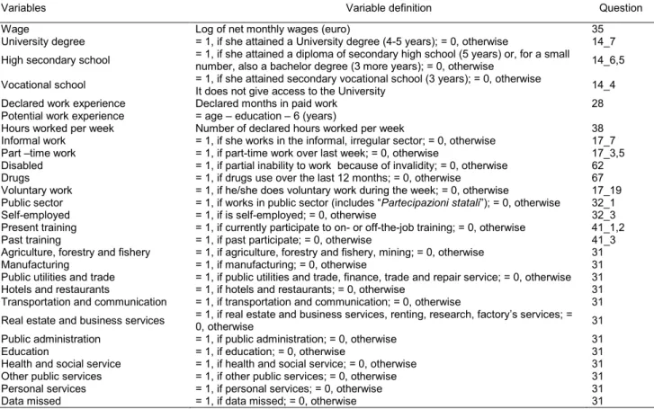
Table I.1 in the Appendix documents the definition used for the variables whose name is not self-evident. Note that declared work experience (measured in months) is preferred to potential work

experience as a more accurate proxy6 _{for the actual underlying}

characteristics. As noted also in Altonji and Blank (1999), potential work experience overstates the actual years of working, especially in the case of women, which tend to leave the labour market for maternity reasons. In the case of Italy, where unemployment spells are frequent and prolonged, especially among young people, the bias typical of potential work experience is expected to be even greater than elsewhere. Work experience is included also as a quadratic term to capture the possible concavity of the earnings profile.

There is a long tradition of using family background information to control for unobserved ability in studying the earnings profile of young people (see for a survey Card, 1999). The YUSE data set provides

5 _{Notice that wages in brackets are in euro (€ 1 = It.£ 1936.27). This means that the average} wage in our sample is about It.£ 802,800.

information on the parents’ credentials (high school diploma and University degree) and employment status. These variables are used here to identify the possible effect of the family background of young people on their earnings.

4. Results

4.1. Augmented earnings equations

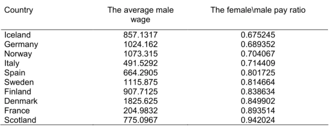
Our findings provide evidence of the existence of a sizeable gender wage gap among young Italian people and of remarkable discrimination that young women experience especially in the Southern regions. The female/male pay ratio among young people in Italy is at 0.71, a figure that is not different from that found in the previous literature, perhaps a little bit lower (Lucifora and Reilly, 1990; Flabbi, 2001). In the South the gap is particularly high: young women earn 73% of men’ wages in Veneto, but only 60% in Campania. Table 1 provides information on the gender pay ratio in all the countries included in the YUSE data. Italy’s female/male pay ratio is one of the highest in the YUSE data, lower only than that in Iceland, Germany and Norway. In Campania, though, women fare worse than in any other country in this group.

[Table 1 about here]

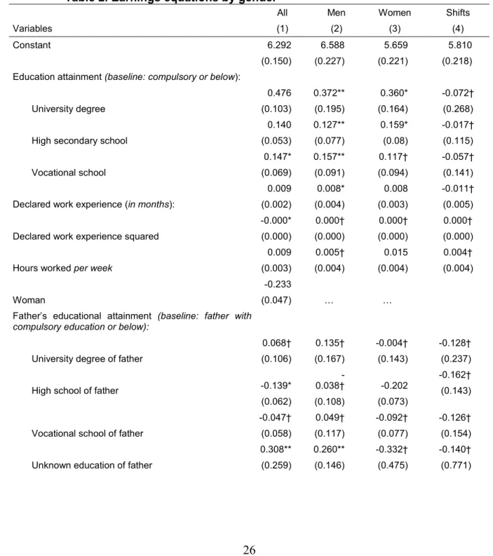
Table 2 reports the results of augmented earnings equations for all young people (column 1) and then separately for men (column 2) and women (column 3). Column 4 contains the coefficients’ shifts of the variables for women in pooled regressions, to test for differences in the coefficients between men and women. The coefficient of the constant term in column 2 measures the average wage of an able-bodied young (18-24) man with compulsory education or below, with poor family background, employed in a formal full-time job in the private construction industry, living in Naples and using no drugs.

[Table 2 about here]

The overall performance of the model is satisfactory with the

adjusted R2 _{reaching the value of 0.46 in the pooled estimate, 0.52 for}

ability of the human capital model to explain these types of estimates is lower for men. The variables have always the expected sign. Not surprisingly, the coefficient for squared work experience is not

significant: in fact, all the individuals in the sample are new entrants7_.

As discussed in more detail later, the unconditional gender wage gap is sizeable at about 33.2% of the average wage. The gap is in the Southern region (51.7%) almost double that in the Northern region

(30.8%), where the average wage is much higher8_{. After controlling for}

all the variables, there still remains a significant wage differential between young women and men amounting overall to 23.3%. The comparable figure is 32.9% in Campania and 8.5% in Veneto. Experimenting with the variables shows that the main contribution to the reduction in the gender coefficient takes place simply adding educational variables. The conditional gender gap obtained from a specification which includes the educational variables only goes down to 23% for the entire sample, to 42% for Campania and to 10% for Veneto. In the case of Campania, a reduction down to 35% is obtained adding variables for family background and other personal characteristics. The rest of the reduction in the coefficient is due to industry dummies.

Confirming expectations based on the human capital theory, having a university qualification significantly and positively influences wages,

providing a premium of about 47.6% of the average wage of workers

with compulsory education or below. This implies that every year of additional education for people with a university degree gives about

7 _{Also the following variables were not statistically significant and were therefore omitted: job} tenure, the parents’ type of occupation, financial support from the family, foreign nationality and the habit of drinking alcohol.

8 _{To make the estimates comparable to those presented in other studies, we follow the} common practice of interpreting the estimated coefficients of dummy variables directly as semi-elasticity. However, following Halvorsen and Palmquist (1980), the coefficients of independent dummy variables in semilog regressions do not represent elasticities. To obtain the semi-elasticity, which measures in this case the percentage change in the median wage, the following formula should be used:

(

e

β

−

1

)

∗

100

. In this terms, the unconditional gender wage gap equals 39.4% overall, 36.1% in Veneto and 67.7% in Campania.

5.3% higher average wages compared to people with compulsory

education only9_.

Recall from a previous section that the general finding of the literature on the magnitude of returns to education for women in Italy is mixed (Dell’Aringa, Ghinetti and Lucifora, 2000), while for most OECD countries, women’s returns to education are higher than men’s (Psacharopoulos, 1985 and 1994). In the YUSE data, young women’s returns to education are almost the same as those of men for university education, are higher in the case of high secondary and lower in the case of vocational school, similar to what Checchi (2002) finds. However, column 4 suggests that the differences are not statistically significant.

Men with a university degree receive about 37% higher wages from their job than their colleagues with compulsory education only. The comparable figure for women is only slightly lower, at 36%. Each year of education for young women and men with a university degree gives about 4% higher wages compared to gender groups with compulsory education only. These figures are comparable with those found in existing similar studies.

As noted in Card (1999), children’ schooling outcomes are very highly correlated with the characteristics of their parents, and in particular with the parents’ education. As expected, the estimated coefficients on the parental education variables are generally well behaved and also in some cases statistically significant. Having a mother with high secondary school diploma provides around 14.5% higher wages for both gender groups. The parents’ university degree is statistically insignificant, which would appear inconsistent with expectations based on economic theory. However, among employed

9 _{This estimate is obtained dividing the coefficient for university education by the nine years} that are necessary to obtain a university degree after finishing compulsory education according to the official curricula:

c u u

Y

Y

r

−

=

β

. Multiplying this value by 100 gives the percentage change for every year of additional education. In Italy, 4-5 years are necessary to attain a university degree, according to the type of degree, 5 years to attain a diploma of secondary high school and 3 years to attain a bachelor degree. Two notes of caution are necessary here. First, there is no way in the YUSE data to distinguish the type of University degree. Moreover, it is well-known that the average time actually spent to attain a University degree (about 6-7 years on average) is much bigger than that officially foreseen. This might lead to overestimate the returns to education.

workers only the parents of few have a university degree. Taking into consideration the theory that more educated parents are more likely to invest in their child’s education as a consequence of their own educational experience, one can find that young people of more educated parents at the age between 18 and 24 in Italy are not working

but still studying and are not included in the sample of paid workers10_.

Another way to test for the role of family background on youth wages is to apply sample selection procedures and use family background as independent variable in the participation equation. A maximum likelihood test for sample selection bias was carried out using various baseline groups: group one included all the rest of the sample; group two included only those in education; group three only those unemployed. In all these cases, no evidence of sample selection bias was found. The results, which are available on request, suggest no impact of parents’ education on educational and participation decisions. Also the coefficients in the main equation remain unchanged.

Extensive literature points to the role of work experience as an important component of employability, especially for young people. In addition, education and work experience tend to be inversely related, particularly among young workers, as the higher is the level of education, the lower is the level of general and job-specific skills. As expected, in our estimates the results indicate strong evidence of the length of work experience on wages. For every additional month of work experience, the average individual obtains 1% higher wages. The return to work experience is similar by gender since all individuals are new entrants in the labour market.

Past or present participation in training programmes is almost insignificant and negatively correlated with the level of wages for young people. This result is not surprising, considering that our sample comes from registration at the local employment office and might be expected to contain people “less fortunate” at the labour market. Also training systems may be ineffective. In Italy, training is closer to general education than to work-based training, which might be the reason of unsuccessful scheme’s policy. Also our findings confirm existing doubts

10 _{Consider that 6-7 years on average are necessary to obtain a University degree in Italy} and the YUSE sample is no exception under this respect.

in the literature on whether training is a good instrument for improving young people’s labour market skills (O’Higgins, 2001, p.96).

Voluntary work is negatively correlated with wages. Participation in voluntary work during the week of the interview decreases the average wage by about 1%. As for men it is not significant and decreases the earnings of women by about 14.5%.

As expected, weekly hours of work are significantly and positively correlated with wages: one more hour of work per week gives about 1% increase in the monthly wage. This variable strongly influences the wage differential among women who generally work less (on average 8 hours per week less than men) and it is insignificant for men. Consequently, part-time occupations are very strongly and negatively correlated with wages (especially the men’s average wages). Young part-time working people earn on average 32.2% less than full-time workers (men almost 44% less and, not surprisingly, for women this variable is insignificant).

Working in a state or private sector is not significant for young people. Being self-employed means earning less than in the private sector by about 13%.

Employment in particular types of industries influences the wage differentials between individuals. For all industrial categories, differentials are relatively wider for women. Generally, people working in almost all the sectors considered earn more than those employed in construction, which is taken as a baseline. As expected in the public services young workers earn 13.5% less.

Being partially disabled has a statistically insignificant effect on wages. Those who are taking drugs earn less by about 14%.

Living in the Northern region increases the wages among young people and increases it even twice among women. Women living in Veneto earn on average about € 481, over 49% more than women in Campania, whereas men’s average wage is € 655 in Veneto, which is about 37% higher than in Campania.

Overall, column 4 shows that most of the differences in coefficients between men and women regards the coefficient of the constant term, which suggests that the main differences between men and women are

for the lowest categories of earnings, relative to the least educated men

and women11_.

4.2. Decomposing the gender wage gap

Using the estimations of the previous section, this section calculates Oaxaca and Ransom (1994) mean wage decomposition according to the econometric procedure described in section 2. Table 3 reports this decomposition for the entire sample. Column (1) shows the female-dummy coefficient that is based on a regression in which no other explanatory variable is used. Column (2) includes the main parameter estimates from the specification reported in column one of Table 2, while the columns (3) and (4) provide average characteristics

for men and women, respectively12_{. The following columns measure the}

differences in characteristics between men and women (column 5) and the absolute and relative contribution (column 6 and 7) of each variable to the gender pay gap. Table 6 provides summary figures of the relative contribution of the five groups of explanatory variables used.

[Table 3 about here]

As the final column in Table 3 indicates, about 70% of the overall gender wage gap is due to gender differences in wages that remain after controlling for all available explanatory characteristics.

Personal characteristics like education, work experience or health status increase the overall gender wage gap by about 2%, which is essentially caused by the higher number of better educated women participating in the labour market. Almost 70% of women and only 44% of men have high secondary school education (at other levels of education the shares by gender are similar). Also location increases the overall pay gap by about 21%, due to the higher number of women that are located in high wage regions. Over 42% of the overall gap is explained by individual work effort like weekly hours of work, which confirms that also young women prefer part-time jobs (in the sample almost 50% of women work part-time, which compares to a share of 26% of men). The high share of young people working part-time also

11 _{This hypothesis will be tested by means of quantile regression analysis in future research.} 12 _{The mean of the dummy variables from table 2, 3 and 4 are interpreted as the relative} sample proportions.

depends on the recent diffusion of atypical contracts in Italy. Differences in the type of industry and job explain almost 11% of the pay differential. Over 50% of women are employed in low-paid industries: 24.6% work in the public services, where the average wage is 13.5% lower than wages in the construction industry and 23.3% of them work in public utility and trade where wages are also lower. Men are almost equally distributed across industries.

The wage gap decomposition is different in the two considered

regions (Table 4 and 5). The adjusted R2 _{for pooled regressions relative}

to Veneto and Campania are 0.66 and 0.33 respectively. As the final column of table 4 suggests, in the Southern Campania almost 63.6% of the overall pay gap remains unexplained so that the potential scope for suggesting the existence of gender pay discrimination appears high. The overall gender wage difference is lower in Veneto, in which case only 28% of the gap remains unexplained.

[Table 4 and 5 about here]

Column 2 and 3 of Table 6 reports that generally the explanatory percentage of each group of variables is different from one region to the other. Over 64% of the overall wage gap is explained by individual work effort in Veneto and only 21% in Campania, which depends on a lower individual work effort on the side of women in the North compared to the South. The type of industry and of job explains almost 19% of the gap in Veneto, where over 50% of women are occupied in public low-pay

industries and only 11% in Campania, which suggests that industry

segregation in this region is less important. Only in public services there is a significant gender difference (23.6% of the fraction of women and 11% of the fraction of men), whereas in other industries the percentage

of labour market participation by gender is relatively similar. The

remaining 11% in the North is to be attributed to higher levels of human capital accumulation (7%) and to better family background (4%) on the side of women. In the South these characteristics explain 4.5% of overall gender wage gap.

5. Discussion

The exhibited results are comparable with those of previous studies and suggest that the gender wage differentials are sizeable and similar to those relative to other European countries also for young people. Although this research does not focus on the segregation problem, some points should be stressed.

Considering occupational segregation, which is measured by the fraction of women in a particular industry, one can observe a higher and more persistent concentration of women in low paying industries in the Northern region. Almost 50% of young women are employed in public services, a share which is comparable with the results for prime-aged people in 1996 (Flabbi, 2001). This persistence might suggest that women are systematically excluded (or this is the result of a voluntary decision) from many better paid industries and even at the beginning of their career they choose the least paid occupations.

It is also worth noting that in industries where the proportion of women is high (for example public utility and trade or public services) men’s wages are lower than those of other males and female coefficients are flatter. These results suggest that women’s occupational segregation and also intensity seems to play an important role as far as wage determination is concerned and might be considered as an additional characteristic able to capture wage differentials (Lucifora, Reilly, 2000).

Another finding is the high participation of young highly educated women in the labour market. About 70% of women from the sample achieved at least a high school diploma and this fraction is higher than that of men (44%), which is the cause of an increase in the overall gender wage gap by about 2%. These results confirm that women with higher educational levels are more likely to participate in the labour market and may raise the question about the potential selectivity bias through the labour force participation decision also mentioned in the literature about Italy (see Flabbi, 2001, p.384). In fact, following Vella (1998, p.129) the possibility of sample selection bias arises whenever one examines a sub sample and the factors determining inclusion in the sub sample are correlated with the unobservable variables influencing the variable of primary interest (in our case, wages). The potential

selectivity problem could cause an upward bias in the estimates of the

ceteris paribus gender wage gap. We tested this hypothesis and found no evidence of sample selection bias, which is in line with the finding of similar returns to education of men and women. This analysis might also suggest that the concentration of women in some low pay industries comes earlier than that into inactivity.

Concluding remarks

This paper aimed to investigate the determinants of the gender wage gap among young people in Italy and also to analyse the differences between the Northern and Southern areas. The starting point of the analysis is that while gender differences in wages have been slightly narrowing over the past two decades, they are still significant and persistent in Italy. The adopted modelling strategy, namely Mincerian estimates and the Oaxaca and Ransom decomposition procedure, makes our analysis comparable to others.

The findings of this paper provide evidence of the existence of an overall gender wage gap among young Italian people which is sizeable at about 33.2% of the average wage. This figure is similar to that found in existing studies for adult people. After controlling for all the available variables, there still remains a significant wage differential between young women and men amounting to 23.3%, which is higher than the

general ceteris paribus gender wage gap generally found for

prime-aged women in Italy (16-17%).

Other findings of the paper are as follow. The gender wage gap decomposition and the characteristics’ relative contribution indicate that about 70% of the overall wage gap is due to gender differences in wages that remain after controlling for all the observed characteristics. The evidence from the most influential characteristics in the overall gender wage gap’s explanation indicates that, on average, young women tend to work less than men (over 43% of the overall gender wage gap is caused by a lower individual work effort on the side of women), while being segregated in low-pay industries, particularly public services or public utility and trade (almost 11% of the overall gender wage gap is explained by industry segregation).

Controlling for the same characteristics in the Southern and Northern regions produces substantially different results. In the South, the potential scope for gender pay discrimination appears high, whereas the overall gender wage difference is lower in the North. The individual work effort on the side of women relatively to men is lower in the North than in the South and the effect of industry segregation is relatively stronger in the Northern regions.

Finally, the similarity of the findings of this paper with other studies suggests that despite the small size, the YUSE sample can be considered close to a nationally representative statistical sample and allows making further estimations. While beyond the scope of this study, future research will need to focus on female occupational segregation, the endogeneity of schooling decisions and the selectivity problem. All these factors could contribute to reduce the conditional wage gap estimated in this study. A further natural extension of this study will be comparing the case of Italy with that of other EU countries in the YUSE data bank.

Appendix of Tables and Figures

Table 1. The female\male pay ratio (monthly wages, 1998)

Country The average male

wage

The female\male pay ratio

Iceland 857.1317 0.675245 Germany 1024.162 0.689352 Norway 1073.315 0.704067 Italy 491.5292 0.714409 Spain 664.2905 0.801725 Sweden 1115.875 0.814664 Finland 907.7125 0.838634 Denmark 1825.625 0.849902 France 204.9832 0.893514 Scotland 775.0967 0.942024 Note: Monthly wages in euro.

Table 2. Earnings equations by gender Variables All (1) Men (2) Women (3) Shifts (4) Constant 6.292 (0.150) 6.588 (0.227) 5.659 (0.221) 5.810 (0.218)

Education attainment (baseline: compulsory or below):

University degree 0.476 (0.103) 0.372** (0.195) 0.360* (0.164) -0.072† (0.268)

High secondary school

0.140 (0.053) 0.127** (0.077) 0.159* (0.08) -0.017† (0.115) Vocational school 0.147* (0.069) 0.157** (0.091) 0.117† (0.094) -0.057† (0.141)

Declared work experience (in months):

0.009 (0.002) 0.008* (0.004) 0.008 (0.003) -0.011† (0.005)

Declared work experience squared

-0.000* (0.000) 0.000† (0.000) 0.000† (0.000) 0.000† (0.000)

Hours worked per week

0.009 (0.003) 0.005† (0.004) 0.015 (0.004) 0.004† (0.004) Woman -0.233 (0.047) … …

Father’s educational attainment (baseline: father with

compulsory education or below):

University degree of father

0.068† (0.106) 0.135† (0.167) -0.004† (0.143) -0.128† (0.237)

High school of father -0.139*

(0.062) -0.038† (0.108) -0.202 (0.073) -0.162† (0.143)

Vocational school of father

-0.047† (0.058) 0.049† (0.117) -0.092† (0.077) -0.126† (0.154)

Unknown education of father

0.308** (0.259) 0.260** (0.146) -0.332† (0.475) -0.140† (0.771)

Mother’s educational attainment (baseline: mother with compulsory education or below):

University degree of mother -0.081†

(0.148) -0.191† (0.244) -0.033† (0.171) 0.214† (0.329)

High school of mother

0.145* (0.062) 0.132† (0.106) 0.159* (0.08) 0.052† (0.145)

Vocational school of mother

0.133* (0.058) 0.074† (0.113) 0.155* (0.07) 0.094† (0.143)

Unknown education of mother

0.261† (0.259) 0.335† (0.268) 0.160† (0.598) -0.194† (1.012)

Informal work (baseline: formal work)

-0.119 (0.046) -0.020† (0.064) -0.183 (0.065) 0.042† (0.091)

Part–time work (baseline: full time work)

-0.322 (0.09) -0.436 (0.147) -0.177† (0.12) 0.053† (0.062) Disabled 0.152† (0.096) 0.143† (0.119) 0.180† (0.14) 0.035† (0.205) Drugs -0.143* (0.059) -0.177* (0.088) -0.035† (0.075) -0.260† (0.163)

Voluntary work (during the last week)

-0.09* (0.043) -0.060† (0.058) -0.145* (0.066) -0.045† (0.143)

Kind of occupation (baseline: private sector, including

non-profit organisations) State sector 0.023† (0.13) -0.073† (0.211) 0.045† (0.162) 0.196† (0.297) Self-employment 0.131** (0.073) -0.136† (0.102) -0.119† (0.105) 0.036† (0.158)

Training participation (baseline: non-participation to training): Present training -0.177† (0.122) -0.427* (0.177) -0.010† (0.156) 0.408† (0.26) Past training -0.017† (0.064) -0.082† (0.092) 0.042† (0.087) 0.146† (0.139)

Industry (baseline: construction):

Agriculture, forestry and fishery

0.214† (0.162) 0.161† (0.221) 0.288** (0.161) 0.152† (0.417) Manufacturing -0.021† (0.108) -0.106† (0.116) (dropped) (dropped)

Public utility and trade

-0.008† (0.061) -0.130† (0.089) 0.109† (0.092) 0.201† (0.137)

Hotels and restaurants

0.007† (0.075) -0.027† (0.104) 0.053† (0.102) 0.022† (0.157)

Transport and communication

0.262* (0.109) 0.039† (0.129) 0.784 (0.21) 0.709* (0.278)

Real estate and business services

-0.033† (0.097) -0.076† (0.123) 0.060† (0.142) 0.090† (0.208) Public administration 0.159† (0.149) 0.165† (0.263) 0.300** (0.166) 0.009† (0.352) Education 0.063† (0.129) -0.105† (0.221) 0.212† (0.168) 0.214† (0.307)

Health and social service

0.14† (0.11) 0.031† (0.18) 0.297* (0.13) 0.222† (0.240)

Other public services

-0.135† (0.082) -0.223† (0.149) -0.015† (0.102) 0.151† (0.193) Personal services 0.092† _- 0.319* 0.293†

(0.113) 0.075† (0.291) (0.143) (0.397) Data missed 0.054† (0.298) -0.531† (0.471) 0.474 (0.163) (dropped)

Location (baseline: Neaples):

Verona 0.463 (0.066) 0.247* (0.106) 0,670 (0.092) 0.377* (0.147) Vicenza 0.632 (0.079) 0.396 (0.138) 0,856 (0.106) 0.476* (0.198) Belluno 0.293 (0.07) 0.179** (0.108) 0,477 (0.093) 0.220† (0.165) Treviso 0.441 (0.0.09) 0.323* (0.128) 0,572 (0.119) 0.239† (0.186) Venezia 0.537 (0.062) 0.387 (0.093) 0,697 (0.09) 0.277* (0.136) Padova 0.444 (0.066) 0.389 (0.126) 0,593 (0.09) 0.198† (0.166) Rovigo 0.451 (0.082) 0.280 (0.108) 0,634 (0.115) 0.292** (0.171) Caserta 0.014† (0.131) -0.042† (0.184) 0,087† (0.139) 0.206† (0.247) Benevento 0.204† (0.217) 0.254† (0.355) 0,138† (0.125) -0.271† (0.477) Avellino 0.201† (0.143) 0.056† (0.197) 0,341 (0.127) 0.338† (0.292) Salerno 0.017† (0.085) 0.004† (0.129) 0,052† (0.123) -0.006† (0.192) Number of observations 746 372 374 746 Number of variables 47 46 45 92 R2 0.50 0.41 0.58 0.99 Adj-R2 _{0.46 0.33 0.52 0.99}

Modified R2 _{0.46 0.36 0.51 0.87}

Notes: 1) Dependent variable is the log of net monthly wages;

2) Heteroscedastic-consistent asymptotic standard errors (Huber-White) are in parentheses;

3) The statistical significance for all reported estimates is as follows: nothing stands for

statistically significant at the 1% level; * for statistically significant at the 5% level;** for

statistically significant at the10% level; † for statistically not significant;

4) Column 4 contains the coefficients of the variables for women in pooled estimates. They represent the shifts of coefficients with respect to the average. The estimate allows for different constant terms for men and women. The reported constant is the coefficient of a dummy for women;

5) For further information on the definition of variables, see Appendix 1.

6)

(

)

(

)

(

n

k

)

n

R

R

Adj

−

−

−

−

=

−

2

1

1

2

1

_{, whereas} 2 _{1 R}2 n k R Modified _      ₋ = −

31

T abl e 3. Wage gap dec o mposit ion V ari abl es Coef fici ent es tima te (1) Coef fici ent es tima te (2) Xm (3) Xf (4) M ean di fferenc e : m en-w om en (5) A bs olu te c ont ribut io n t o w age gap (2)* (5) Rel at ive c on tri w age gap (2)* (5)/ (1) Uni vers ity degree … 0. 476 0. 008 0. 008 0. 000 0. 000 Hi gh s ec ondary sc hool degree … 0. 140 0. 444 0. 698 -0. 254 -0. 036 V oc ati onal s chool … 0. 147 0. 116 0. 088 0. 027 0. 004 Dec lared w ork e xperi enc e (in m ont hs ) … 0. 009 26. 478 22. 618 3. 861 0. 033 Dec lared w ork e xperi enc e squared … 0. 000 1285. 984 961. 254 324. 730 -0. 014 Hours w ork ed per w ee k … 0. 009 36. 911 29. 179 7. 732 0. 068 W om an -0. 332 (0. 049) -0. 233 0. 000 1. 000 -1. 000 0. 233 Uni vers ity degree of f at her … 0. 068 0. 065 0. 088 -0. 024 -0. 002 Hi gh s ec ondary sc hool degree of f ather … -0. 139 0. 239 0. 265 -0. 025 0. 004 V oc ati onal s chool of f ather … -0. 047 0. 073 0. 096 -0. 024 0. 001 Unk now n educ at ion of f ather … -0. 308 0. 035 0. 016 0. 019 -0. 006 Uni vers ity degree of m ot her … -0. 081 0. 032 0. 064 -0. 032 0. 003 Hi gh s ec ondary sc hool degree of m other … 0. 145 0. 207 0. 209 -0. 002 0. 000 V oc ati onal s chool of m other … 0. 133 0. 062 0. 094 -0. 032 -0. 004 Unk now n educ at ion of m other … 0. 261 0. 024 0. 013 0. 011 0. 003

32

In fo rm al w ork … -0. 119 0. 301 0. 345 -0. 044 0. 005 P art – tim e w ork … -0. 322 0. 261 0. 492 -0. 231 0. 074 Di sabl ed … 0. 152 0. 062 0. 029 0. 032 0. 005 Drugs … -0. 143 0. 231 0. 075 0. 156 -0. 022 V olunt ary w ork … -0. 091 0. 508 0. 725 -0. 217 0. 020 S tat e s ect or … 0. 023 0. 056 0. 056 0. 000 0. 000 S elf -e m plo ym en t … -0. 131 0. 164 0. 219 -0. 055 0. 007 P res ent t rai ni ng … -0. 177 0. 040 0. 067 -0. 027 0. 005 P ast tr ai ni ng … -0. 017 0. 102 0. 099 0. 003 0. 000 A gri cu lture, fo rest ry and fis hery … 0. 214 0. 019 0. 005 0. 013 0. 003 M anuf ac tu re … -0. 022 0. 094 0. 000 0. 094 -0. 002 P ubl ic ut ilit y and t rade … -0. 008 0. 226 0. 233 -0. 007 0. 000 Hot els and rest aurant s … 0. 007 0. 169 0. 118 0. 052 0. 000 Trans port and co m m uni ca tion … 0. 262 0. 067 0. 021 0. 046 0. 012 Real es ta te and bu sine ss se rv ic es … -0. 033 0. 078 0. 091 -0. 013 0. 000 P ubl ic ad m ini st rat ion … 0. 159 0. 027 0. 027 0. 000 0. 000 E duc at ion … 0. 063 0. 030 0. 056 -0. 027 -0. 002 Heal th and s oc ia l s ervi ce … 0. 140 0. 005 0. 032 -0. 027 -0. 004 Ot her publ ic s ervi ces … -0. 135 0. 099 0. 246 -0. 147 0. 020 P ers onal s ervi ce s … 0. 092 0. 008 0. 067 -0. 059 -0. 005 Dat a m iss ed … 0. 054 0. 005 0. 008 -0. 003 0. 000 V erona … 0. 463 0. 089 0. 126 -0. 037 -0. 017 V ic enza … 0. 632 0. 030 0. 037 -0. 008 -0. 005 B ell uno … 0. 293 0. 011 0. 024 -0. 013 -0. 004 Trevi so … 0. 441 0. 062 0. 078 -0. 016 -0. 007

33

V enezi a … 0. 537 0. 094 0. 134 -0. 040 -0. 021 -0. P adova … 0. 444 0. 056 0. 088 -0. 032 -0. 014 -0. Rovi no … 0. 451 0. 038 0. 048 -0. 010 -0. 005 -0. Cas ert a … 0. 014 0. 062 0. 029 0. 032 0. 000 0. B enevent o … 0. 204 0. 011 0. 011 0. 000 0. 000 0. A vel lino … 0. 201 0. 027 0. 016 0. 011 0. 002 0. S ale rno … 0. 017 0. 089 0. 115 -0. 026 0. 000 -0. N o tes. C o lum n (1), th e fem a le dum m y estim a te is ba sed on a regres sio n in w h ic h no other expla nator y vari abl es are u se d ; colum n (2), c o va riate poole d -da ta regre ss ion; c o lum n (3) and (4) present th e m

ean for all var

iab le s for m en (Xm ) and w o m en (Xf); heteros cedas tic-con si sten t as ym stan dard errors (Huber-Whit e) are in pare nthe se s. For furt her i n form ati on o n th e varia b le s’ definit ion, see Appe ndix 1. Source : el abora tio n on YU SE data.

34

T abl e 4. Wage gap dec o mposit io n f o r Venet o V ari abl es Coef fici ent es tim at e (1) Coef fici ent es tim at e (2) Xm (3) Xf (4) M ean di fferenc e : m en-w om en (5) Ab so lu te cont ribut io n t o w age gap (2)*(6) cont ribut io n Rel at ive to w (2)* (3)/ (1) nort h Uni vers ity degree … 0. 409 0. 021 0. 010 0. 011 0. 005 Hi gh s ec ondary sc hool degree … 0. 054 0. 546 0. 765 -0. 219 -0. 012 V oc ati onal s chool … 0. 011 0. 163 0. 115 0. 048 0. 001 Dec lared w ork ex peri enc e (in m on ths ) … 0. 006 23. 532 21. 730 1. 802 0. 012 Dec lared w ork ex peri enc e s quared … 0. 000 860. 085 776. 610 83. 475 -0. 005 Hours w ork ed per w ee k … 0. 021 36. 553 29. 635 6. 918 0. 147 W om an -0. 308 (0. 054) -0. 085 0. 000 1. 000 -1. 000 1. 000 Uni vers ity degree of f at her … 0. 026 0. 071 0. 080 -0. 009 0. 000 Hi gh s ec ondary sc hool degree of fa ther … -0. 047 0. 241 0. 250 -0. 009 0. 000 V oc ati onal s chool of fa ther … 0. 016 0. 106 0. 130 -0. 024 0. 000 Unk now n educ at ion of f ather … -0. 076 0. 028 0. 015 0. 013 -0. 001 Uni vers ity degree of m ot her … 0. 290 0. 028 0. 055 -0. 027 -0. 008 Hi gh s ec ondary sc hool degree of m other … 0. 030 0. 220 0. 185 0. 035 0. 001 V oc ati onal s chool of m other … 0. 066 0. 099 0. 135 -0. 036 -0. 002 Unk now n educ at ion of m other … -0. 197 0. 014 0. 005 0. 009 -0. 002 In fo rm al w ork … -0. 137 0. 213 0. 300 -0. 087 0. 012 P art – tim e w ork … -0. 180 0. 156 0. 440 -0. 284 0. 051

35

Di sabl ed … 0. 042 0. 071 0. 040 0. 031 0. 001 -0. 004 Drugs … -0. 086 0. 305 0. 085 0. 220 -0. 019 0. 062 V olunt ary w ork … 0. 035 0. 539 0. 730 -0. 191 -0. 007 0. 022 S tat e s ect or … 0. 121 0. 064 0. 050 0. 014 0. 002 -0. 005 S elf -e m plo ym en t … -0. 061 0. 064 0. 055 0. 009 -0. 001 0. 002 P res ent t rai ni ng … -0. 135 0. 035 0. 060 -0. 025 0. 003 -0. 011 P ast tr ai ni ng … -0. 073 0. 092 0. 090 0. 002 0. 000 0. 001 A gri cu lture, fo rest ry and fis hery … -0. 004 0. 028 0. 010 0. 018 0. 000 0. 000 M anuf ac tu re … -0. 149 0. 092 0. 000 0. 092 -0. 014 0. 044 P ubl ic ut ilit y and t rade … -0. 012 0. 227 0. 275 -0. 048 0. 001 -0. 002 Hot els and rest aurant s … -0. 176 0. 113 0. 155 -0. 042 0. 007 -0. 024 Trans port and co m m uni ca tion … 0. 197 0. 057 0. 010 0. 047 0. 009 -0. 030 Real es ta te and bu sine ss s ervi ces … -0. 033 0. 092 0. 095 -0. 003 0. 000 0. 000 P ubl ic ad m ini st rat ion … 0. 130 0. 043 0. 035 0. 008 0. 001 -0. 003 E duc at ion … -0. 091 0. 007 0. 040 -0. 033 0. 003 -0. 010 Heal th and s oc ia l s ervi ce … 0. 137 0. 000 0. 020 -0. 020 -0. 003 0. 009 Ot her publ ic s ervi ces … -0. 228 0. 078 0. 255 -0. 177 0. 040 -0. 131 P ers onal s ervi ce s … (dropped) 0. 000 0. 000 0. 000 0. 000 Dat a m iss ed … (dropped) 0. 000 0. 000 0. 000 Not es : Col um n (1), t he f em ale dum m y es tim at e i s bas ed on a regres sion i n w hic h no ot her ex pl anat ory v ari abl es are us ed; c olu m n (2), c ov ari at es i n pool regres sion; c olu m n (3) and (4) pres ent t he m ean f or al l v ari abl es f or m en (X m ) and w om en (X f); het erosc ed as tic -c on sis ten t asy m pt ot ic st an da rd errors (Huber -W hi te parent hes es. For fu rt her in fo rm at ion on t he v ari abl es ’ def in ition, s ee A ppendi x 1. S ourc e: el aborat ion on Y U S E dat a.

36

T abl e 5. Wage gap dec o mposit io n f o r Campa n ia Variab les Coeffi cien t esti mat e (1) Coeffi cien t esti mat e (2) Xm (3) Xf (4) M ean differ enc e: men-w o men (5) Abs o lu te contr ibut ion to w age gap (2)* (3) Re la contr ibut w age gap (2)* (3)/(1) U n iv ersity de gree … 0.633 0.000 0.006 -0.006 -0.004 H igh s e co ndary s ch o ol degr e e … 0.177 0.381 0.621 -0.240 -0.042 Vocat iona l s cho ol … 0.117 0.087 0.057 0 .029 0.003 D e clar ed w o rk ex perien ce (in m onths) … 0.012 28.27 7 23.63 8 4 .639 0.056 D e clar ed w o rk ex perien ce squ a red … 0.000 1545. 948 1173. 489 372.4 5 9 -0.025 H ours w o rked per w eek … 0.005 37.13 0 28.65 5 8 .475 0.044 W om an -0.517 (0.0 68) -0.329 0.000 1.000 -1.000 0.329 U n iv ersity de gree of f a ther … 0.033 0.061 0.098 -0.037 -0.001 H igh s e co ndary s ch o ol degr e e of fat her … -0.189 0.238 0.282 -0.044 0.008 Vocat iona l s cho ol of fat her … -0.120 0.052 0.057 -0.006 0.001 U n know n edu cat ion of fa ther … -0.459 0.039 0.017 0 .022 -0.010 U n iv ersity de gree of moth er … -0.326 0.035 0.075 -0.040 0.013 H igh s e co ndary s ch o ol degr e e of m o ther … 0.269 0.199 0.236 -0.036 -0.010 Vocat iona l s cho ol of m o ther … 0.136 0.039 0.046 -0.007 -0.001 U n know n edu cat ion of m o ther … 0.547 0.030 0.023 0 .007 0.004 Inform al w o rk … -0.093 0.355 0.397 -0.042 0.004 Part –ti m e w o rk … -0.287 0.325 0.552 -0.227 0.065

37

D isab led … 0.353 0.056 0.017 0 .039 0.014 D rugs … -0.172 0.186 0.063 0 .123 -0.021 Volunt ary w o rk … -0.132 0.489 0.718 -0.229 0.030 State sect or … -0.045 0.052 0.063 -0.011 0.001 Self-e mploy ed … -0.204 0.225 0.408 -0.183 0.037 Presen t trai nin g … -0.210 0.043 0.075 -0.031 0.007 Past tr ain ing … 0.041 0.108 0.109 -0.001 0.000 Agricu ltur e, for e stry a n d fi sh er y … 0.534 0.013 0.000 0 .013 0.007 M a nufacture … 0.071 0.095 0.000 0 .095 0.007 Publi c ut ility a n d tr ade … -0.021 0.225 0.184 0 .041 -0.001 H o tels and res taura n ts … 0.152 0.203 0.075 0 .129 0.020 T ransport a n d co mmu nic a tio n … 0.304 0.074 0.034 0 .039 0.012 R eal e stat e an d bu sin e ss s e rv ic es … -0.087 0.069 0.086 -0.017 0.001 Publi c ad mi nis trati on … 0.223 0.017 0.017 0 .000 0.000 Educat ion … 0.075 0.043 0.075 -0.031 -0.002 H ealth and so cia l s e rv ice … 0.177 0.009 0.046 -0.037 -0.007 O ther pub lic s e rv ice s … -0.030 0.113 0.236 -0.123 0.004 Person al serv ic es … 0.190 0.013 0.144 -0.131 -0.025 D a ta m is sed … 0.153 0.009 0.017 -0.009 -0.001 Not es : Col um n (1), t he f em ale dum m y es tim at e i s bas ed on a regres sion i n w hic h no ot her ex pl anat ory v ari abl es are us ed; c olu m n (2), c ov ari at es i n pool ed-dat regres sion; c olu m n (3) and (4) pres ent t he m ean f or al l v ari abl es f or m en (X m ) and w om en (X f); het erosc ed as tic -c on sis ten t asy m pt ot ic st an da rd errors (Huber -W hi te ) are i parent hes es. For fu rt her in fo rm at ion on t he v ari abl es ’ def in ition, s ee A ppendi x 1. S ourc e: el aborat io n on Y U S E dat a.

38

T abl e 6. Re la ti ve cont ribut io n t o t h e w age gap by group of v ari abl es Italy Veneto C a mpan ia O verall w age gap of w h ich: 0.332 0.308 0.517 E xplaine d c o mp onen ts a (in % ): Person al char acter ist ic s 0.017 0.070 -0.036 Effort -0.427 -0.642 -0.211 Fami ly bac kgro und 0.005 0.039 -0.008 Loca tion 0.213 … … Indu stry and ty pe of job -0.106 -0.189 -0.111 U n ex plained g a p, cet e ris par ib us (i n %) -0.703 -0.278 -0.636 Not e: a P ers onal c harac te ris tic s i nc lude educ at ional at ta in m ent , w or k ex peri enc e, t enure, tr ai ni ng, v olunt ary w or k and heal th ; i ndi vid ual w ork e ffo rt in cludes hour s w per w eek and part -tim e c ont ract ; fa m ily bac kg round i ncl udes educ ati onal at ta in m ent of f at her and m ot her; indus try and t ype of job i nc lude s: f irm s’ ow ners hip , part to t he in fo rm al s ect or, s elf -em plo ym ent and i ndust ry; lo ca tion in cl udes to w n of res iden ce . S ourc e: el aborat ion on Y U S E dat a.

References

ALTONJI, JOSEPH G. and REBECCA M. BLANK, 1999. “Race and Gender in the

Labor Market”, in Ashenfelter, O. C. and D. Card (eds.), Handbook of Labour

Economics, Elsevier Science Publishers BV, Vol. 3c, Chapter 48, pp. 3143-3259.

BECKER, GARY S., 1971. The economics of discrimination, 2nd edition, The University

of Chicago Press, Chicago.

BONJOUR, DOROTHE and LIA PACELLI, 1998. “Wage Formation and the Gender Wage Gap: Do Institutions Matter? Italy and Switzerland Compared”, Discussion

Paper No.12, University College London.

BRUNELLO, GIORGIO, COMI, SIMONA and CLAUDIO LUCIFORA, 2000. “Returns to Education in Italy: A Review of the Applied Literature”, IZA Discussion Paper No. 120.

CARD, DAVID, 1999. “The Causal Effect of Education on Earnings”, in Ashenfelter, O.

C. and D. Card (eds.), Handbook of Labour Economics, Elsevier Science

Publishers BV, Vol. 3c, Chapter 30, pp.1801-1863.

CHECCHI, DANIELE, 2001. “Scuola, Formazione e Mercato del Lavoro”, in Brucchi, L.,

Manuale di Economia del Lavoro, Il Mulino, Chapter 2, pp. 21-56.

DELL’ARINGA, CARLO, GHINETTI, PAOLO, and CLAUDIO LUCIFORA, 2000. “Pay Inequality and Economic Performance in Italy: a Review of the Applied Literature”,

PiEP Project Meeting,London,LSE.

FLABBI, LUCA, 1997. “Discriminazione di Genere e Rendimenti dell’istruzione:

un’analisi su Microdati Individuali”, Rivista di Politica Economica, Vol. 12, No. 3,

pp. 187-234.

FLABBI, LUCA, 2001. “La discriminazione: Evidenza Empirica e Teoria Economica”, in

Brucchi, L., Manuale di Economia del Lavoro, Il Mulino, Chapter 17, pp. 381-408.

GROSHEN, ERICA L., 1991. “The Structure of the Female/Male Wage Differential: Is It

Who You Are, What You Do, or Where You Work? ”, The Journal of Human

Resources ,Vol. 26, No. 3, pp. 457-472.

HALVORSEN, ROBERT and RAYMOND PALMQUIST, 1980. “The Interpretation of

Dummy Variables in Semi-logarithmic Equation.”, American Economic Review,

ILO (1999), Employment Youth: Promoting Employment Intensive Growth, Report for the Regional Symposium on Strategies to Combat Youth Unemployment and Marginalisation.

LUCIFORA, CLAUDIO and FEDERICO RAPPELLI, 1993. “Profili retributivi e carriere:

un’analisi su dati longitudinali”, Rapporto sui Salari, ASAP, pp. 117-161.

LUCIFORA, CLAUDIO and BARRY REILLY, 1990. “Wage Discrimination and Female

Occupation Intensity”, Labour, Vol. 4, No. 2, pp. 147-168.

LUPI, CLAUDIO and PATRIZIA ORDINE, 1998. “Un’analisi della Struttura dei

Differenziali Salari in Italia”, Lavoro e Relazioni Industriali, Vol. 2, pp. 69-109.

MINCER, JACOB, 1970. “The Distribution of Labour Incomes: A Survey with Special

Reference to the Human Capital Approach”, Journal of Economic Literature, Vol.

8, No. 1, pp. 1-26.

O’HIGGINS, NIALL, 2001. Youth Unemployment and Employment Policy: A Global

Perspective, ILO, Geneva.

OAXACA, RONALD. L., 1973. “Male-Female Wage Differentials in Urban Labor

Markets”, International Economic Review, Vol. 14, No. 3, pp. 693-709.

OAXACA, RONALD. L. and MICHAEL R. RANSOM, 1994. “On Discrimination and the

Decomposition of Wage Differentials”, Journal of Econometrics, Vol. 61, No. 1, pp.

5-21.

PRASAD, ESWAR S. and FRANCESCA UTILI, 1998. “The Italian Labour Market:

Stylised Facts, Institutions and Direction for Reform, IMF Working Paper, Vol. 42.

PSACHAROPOULOS, GEORGE, 1985. “Return to Education: a Further international

Update and Implications”, The Journal of Human Resources, Vol. 20, pp. 585-604.

PSACHAROPOULOS, GEORGE, 1994. “Returns to Investment in Education: A Global

Update”, World Development, Vol. 22, No. 9, pp. 1325-1343.

VELLA, FRANCIS, 1998. “Estimating Models with Sample Selection Bias: A Survey”,