Genomic data integration & gene expression analysis of single cells

(1)

Genomic Data Integration

&

Gene Expression Analysis of Single Cells

Dissertation zur Erlangung

des Doktorgrades der Naturwissenschaften (Dr. rer. nat.)

der Fakultät für Biologie und Vorklinische Medizin

der Universität Regensburg

vorgelegt von

Herrn Matthias Maneck M.Sc.

aus

Berlin

im Jahr 2011

(2)

(3)

Die Arbeit wurde angeleitet von:

1. Betreuer: Prof. Dr. Wolfram Gronwald

2. Betreuer: Prof. Dr. Rainer Spang

Unterschrift:

(4)

(5)

(6)

(7)

List of Figures

1.1 Schema of cDNA and high density oligonucleotide arrays. . . 9 2.1 Illustration of cross validation, kernel density estimation and silhouettes. 17 4.1 Inuence of parameters σ and ω on the smoothing process. . . 39

4.2 Illustration of matrix fusion. . . 40 4.3 Diagram of simulation model and exemplary data set. . . 48 4.4 Selection of smoothing parameter σ illustrated on simulated data. . . 49

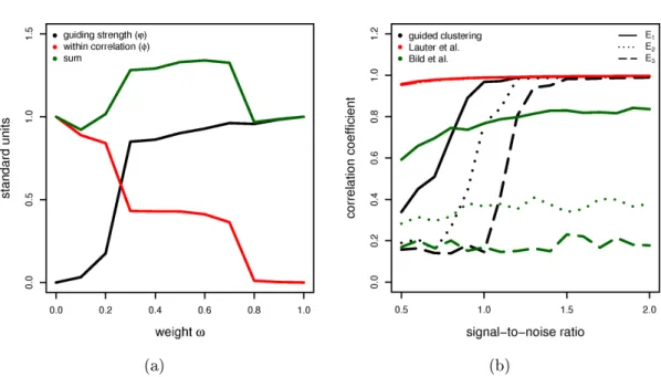
4.5 Automatic selection of parameter ω and comparison of prediction

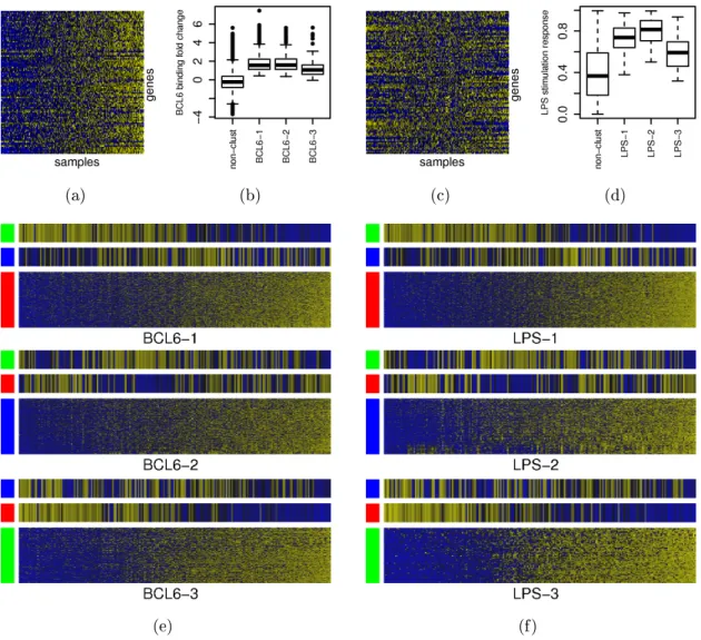
accuracies of guided clustering with other approaches. . . 50 4.6 Extracted gene modules of DLBCL using BCL6 ChIP-on-chip or LPS

stimulation data for guidance. . . 56 4.7 Choice of smoothing parameter σ for BCL6 data. . . 57

4.8 Choice of smoothing parameter σ for LPS data. . . 60

5.1 Scatter plots for color switch experiment and sensitivity evaluation of Cy5 and Cy3 channel. . . 72 5.2 Boxplots illustrating sensitivity and fold change conservation. . . 77 5.3 ROC and classication analysis of the spike-in data set. . . 79 6.1 Classication results of spindle vs. oocytes & zygote vs. Pb2 samples. 89 6.2 Comparison of enriched or depleted genes in Pb2 and spindle samples. 90 6.3 Result of a cluster approach to nd an asymmetric mRNA

distribu-tion within sister blastomeres. . . 93 6.4 Cluster analysis of sister blastomeres based on group separation. . . . 97 6.5 Maternal transcriptome inheritance for 1st, 2nd and 3rd mitotic

di-vision. . . 98 6.6 Cluster analysis of 3-cell sister blastomeres. . . 99

(12)

(13)

List of Tables

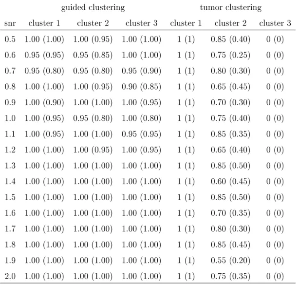
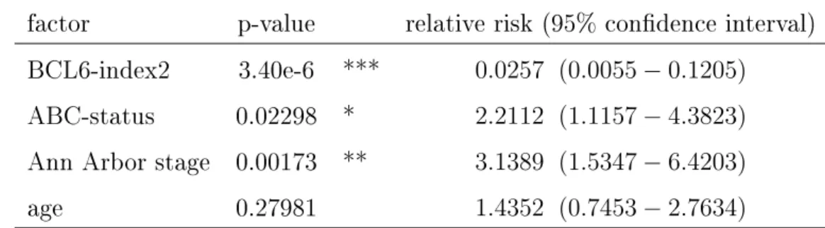
4.1 Signicance analysis of gene modules. . . 51 4.2 Cox-regression analysis of BCL6-index2. . . 55 4.3 Cox-regression analysis of LPS-index2. . . 59 5.1 Estimated copy number per spike-in oligo used for the preliminary

experiments. . . 71 5.2 Estimated copy number per spike-in oligo for the spike-in data set. . . 75 5.3 Analysis results of the spike-in data set. . . 80 5.4 GO-term analysis of arrested vs. stimulated Cal51 and T47D cell line

samples. . . 82 6.1 Gene list BCL6-index2. . . 110 6.2 Gene list LPS-index2. . . 117

(14)

(15)

Abbreviations and Notation

ABC - activated B-cell lymphoma AUC - area under the curve BCL6 - B-cell CLL/lymphoma 6

BP - biological process CC - cellular component cDNA - complementary DNA

CGH - comparative genomic hybridization ChIP - chromatin immunoprecipitation

CV - cross validation

Cy3 - Cyanine-3-dNTP, uorescently labeled DNA (green) Cy5 - Cyanine-5-dNTP, uorescently labeled DNA (red) DLBCL - diuse large B-cell lymphoma

DNA - deoxyribonucleic acid DTC - disseminated tumor cell

FPR - false positive rate GC - germinal center

GCB - germinal center like B-cell lymphoma GO - gene ontology

HL - Hodgkin lymphoma

HMEC - human mammary epithelial cells KDE - kernel density estimation

LPS - lipopolysaccharide MF - molecular function mRNA - messenger RNA

n - number of samples in a gene expression data set

NHL - non-Hodgkin lymphoma xi

(16)

P - a P-value

Padj - a P-value adjusted for multiple testing

PAM - the cluster algorithm partitioning around medoids PAMr - prediction analysis for microarrays

Pb2 - the second polar body

PCR - polymerase chain reaction qPCR - quantitative PCR

r - a correlation coecient rmsd - root mean square deviation RNA - ribonucleic acid

ROC - receiver operator characteristic TPR - true positive rate

tRNA - transport RNA

X, T, G - expression matrices of microarray data sets Y - vector containing sample labels

(17)

Preface

Acknowledgement

This work was accomplished in the Computational Diagnostics Group of the Insti-tute of Functional Genomics of the University of Regensburg in cooperation with the Chair of Experimental Medicine and Therapy Research of the department of pathology of the University Hospital of Regensburg. First and foremost, I thank my supervisors Rainer Spang and Christoph Klein for giving me the opportunity to carry out my research projects in their groups. This gave me the opportunity to work in both, a theoretical bioinformatics group as well as in a clinically oriented lab. I thank all past and present colleagues for the pleasant working atmosphere. Es-pecially I thank my oce mates Benedict, Christian K., Claudio, and Mohammed, as well as Stefan, Juby, Christian H. and Tully from the Computational Diagnos-tics group and Isabell, Anya, Daniel and Sophie from the Chair of Experimental Medicine and Therapy Research for fruitful (non-) scientic discussions.

Above all, I am exceptionally grateful to my girlfriend Corinna, my parents and my brother for their relentless support and love.

(18)

Parts of this thesis have been published in peer-review journals. The guided clus-tering algorithm described in chapter 4 has been published in the Bioinformatics journal (Maneck et al., 2011). Further, the content of chapter 6 has been published in The EMBO Journal (Vermilyea et al., 2011).

Figures

Figures 1.1 and 6.5 have been taken from Jares (2006) and Vermilyea et al. (2011) respectively.

(19)

Cancer is one of the leading causes of death world wide. According to the World Health Organization (WHO) 7.6 million deaths, which is about 13% of all deaths, were the result of cancer in 20081_{. This frightening number is projected to continue}

to rise to over 30 million in 2030. In response the WHO launched its Noncom-municable Diseases Action Plan that focusses on preventing and controlling cancer. Prevention of diseases is of course better than treatment or control. However, cancer treatment is one of the major challenges for present health systems. Eciency and eect of present cancer treatments are mainly linked to an early detection and pre-cise diagnosis. Early detection always involves the patients awareness of early signs and symptoms. A precise diagnosis of cancer is only possible based on tissue biop-sies, which are judged by a pathologist according to morphological and molecular properties.

Another way to investigate molecular characteristics of tumor biopsies, which has been subject to intensive research in recent years, is gene expression proling. In fact, it has been shown by Hummel et al. (2006) that microarray gene expression analysis is able to improve the molecular stratication and classify former unknown cases of lymphoma. We believe that information about expression states of thou-sands of genes measured simultaneously holds even greater potential. This potential can be unlocked if gene expression data is combined with additional data from other experiments that measure specic perturbations on the transcriptome. Such per-turbations might be stimulation of cell lines with certain compounds, knock-out or knock-in of specic genes or binding anities of transcription factors to the DNA. The integration of tumor biopsies with additional experimental data allows the de-tection of gene clusters within the expression proles that respond to perturbations. In this thesis the prospects of data integration in this context are subject of chapters 3 and 4. In chapter 3 we will review the data integration literature with respect to gene expression analysis. This is followed by a detailed description of a novel data integration method developed during this thesis in chapter 4.

Recently the analysis of single cells has moved into the focus of cancer research. The present model of disseminated tumor cell (DTC) and early metastatic spread suggests that single tumor cells disseminate from the primary tumor in a very early

1_{GLOBOCAN 2008, International Agency for Research on Cancer}

(20)

the input of DTCs into cancer research is manifold. For example, the analysis of DTCs could establish new prognostic biomarkers that predict disease recurrence after surgery or identify patients in need of antiproliferative therapy. However, the analysis of single cells raises new technological and analytical challenges as the amount of available sample material is low. Usually clinical samples consist of thou-sands of cells. In this thesis we investigate single cell microarray gene expression proling in chapter 5. We compare the performance of several normalization pro-cedures with respect to dierent applications of gene expression analysis, namely dierential gene expression analysis and classication. An application of single cell microarray analysis is given in chapter 6. There we leave the eld of cancer research and enter reproductive medicine and embryonic research. We analyze samples that naturally consist of only one cell, the murine zygote. We investigate the very rst steps of embryogenesis by comparing the single cells of2−and 3−cell blastomeres. The aim of this analysis is to answer the question whether there exist conserved dif-ferences within the transcriptomes of couplets or triplets derived from2−or3−cell blastomeres.

In the introductory part of this thesis, namely chapter 1 and 2, the biological terms and concepts used throughout this thesis are described. This is followed by an introduction into the machine learning techniques used in data analysis, namely classication, clustering and kernel density estimation.

The thesis closes with a summary and nal conclusions.

(21)

Part I

Introduction

(22)

(23)

We start by introducing the terminological basics and background for the content of this thesis.

In chapter 1 the most important molecular biological terms used are described. This is followed by a description of molecular biological techniques and methods that were used to generate the data sets analyzed in this work. Several textbooks were used for this part of the introduction namely: Basiswissen Biochemie: mit Pathobiochemie (Löer, 2009), Biochemie (Stryer, 1996), Lehrbuch der Molekularen Zellbiolo-gie (Alberts et al., 2005) and Bioinformatics - Sequence and Genome Analysis (Mount, 2004) .

In chapter 2 a brief introduction into the concepts of machine learning methodology used is given. This comprises classication, kernel density estimation and clustering. In this chapter the textbooks The Elements of Statistical Learning (Hastie et al., 2001), Elements of Computational Statistics (Gentle, 2002) and Semi-Supervised Learning (Chapelle et al., 2006) as well as the original publications of Kaufman and Rousseeuw (1990), Rousseeuw (1987) and Tibshirani et al. (2002) were used.

(24)

(25)

Chapter 1 Biological Content

1.1 Molecular Biology

Gene Regulation Each eukaryotic cell contains the whole genome of its specic

organism and has therefore the potential to express all genes. However, only a frac-tion of genes is expressed within a cell in a certain condifrac-tion and time point. Between dierent tissues the set of expressed genes diers. This is called dierential gene ex-pression. It is of crucial importance for all cells to regulate their gene expression in response to variable environmental conditions. In eukaryotic cells the regulatory mechanisms vary from the inactivation of genes by methylation via mRNA editing or degradation to transcription factors. Within an organism the cells interact and gene regulation is controlled and triggered by a complex network of signals.

Transcription Factors Transcription factors are molecules that can bind to spe-cic DNA sequences. They can either activate or repress the process of transcription and are part of the gene regulation machinery.

Dierentiation & Proliferation Highly specialized tissues are responsible for dierent requirements of an organism. The lungs are responsible for the oxygen absorption, the muscles for movement and the intestine for the absorption of nu-trients. However, all the cells of an organism develop out of a single fertilized egg. As an organism develops many cells are needed and the number of cells increases via cell division. This increase of cell numbers is called proliferation. In chapter 6 we investigate the very rst cell divisions by analyzing single cells from 2- and 3-cell mice blastomeres and zygotes. In contrast, dierentiation is the process that

(26)

specialize a cell to a certain biological task.

Cancer Cancer is a group of diseases characterized by uncontrolled cell prolifer-ation. The disease is based on the accumulation of mutations within a single cell. These mutations result in a breakdown of the normal regulatory control mechanisms. Mutations can be caused by errors during DNA replication, contact with harmful chemicals, exposure to radiation or be inherited. Tumors can be developed in all types of tissues and are usually named based on their cellular origin. A tumor can spread to other parts of the body. This process is called metastasis.

Oncogenes & Tumor Suppressor Genes Genes can be directly involved in the

formation of cancer. One distinguishes between oncogenes and tumor suppressor genes. Oncogenes are mutated genes that contribute to the development of a can-cer. They often code for signaling proteins that are involved in the regulation of cell division. In their mutated form they produce a constant stimulus that drives the cell to proliferate. Tumor suppressor genes work in the opposite direction of oncogenes. They code for proteins that keep the cell division under control. However, if a tumor suppressor gene is mutated the control mechanism can not be maintained. This loss of control over cell division may contribute to the development of a cancer. Iden-tication of onco- and tumor suppressor genes is the key to understanding cancer. Their regulation and protein products are interesting targets for drug development and therapies.

Lymphoma Lymphoma are a type of blood or hematopoietic cancer that can

be developed in many parts of the body, including the lymph nodes, spleen, bone marrow and blood. They occur when lymphocytes, a type of white blood cells, proliferate abnormally. The collective term lymphoma contains many subtypes of this disease. There are two main types of lymphoma, the Hodgkin lymphoma (HL) and the non-Hodgkin lymphoma (NHL). The NHL are further classied by their cell of origin. This cell is either a B- or T-lymphocyte, thus the respective lymphoma is referred to as B-cell or T-cell lymphoma. B-cell lymphomas comprise about95% of all lymphomas. In chapter 4 we analyze data from two aggressive forms, the diuse large B-cell lymphoma (DLBCL) and the Burkitt lymphoma. While the data set contains samples from both subtypes the analysis focusses on the DLBCL. We investigate the inuence of the transcription factor BCL6 on the transcriptome, since BCL6 is a key oncogene in the development of DLBCL.

(27)

Cell Lines Cells can be grown separated from the original tissue under con-trolled conditions. This technique is called cell culture. Permanently established cell cultures that can proliferate indenitely are called cell lines.

In cancer research cell lines derived from tumors are widely used as model organ-isms. They are exposed to newly developed drugs or other compounds to test their eects. Another application is the investigation of transcriptome changes given a certain perturbation. This perturbation can be a silenced or activated gene or the application of a specic compound that will activate or block receptors. Then the transcriptome of perturbed cells is compared with control cells without the pertur-bation using gene expression microarrays. Such experiments give new insights into the regulatory mechanism triggered by the perturbation. In this work data from cell line experiments is integrated with gene expression proles of lymphoma patients in chapter 4. Further we used cell lines to generate the expression data employed in the evaluation of singe cell gene expression analysis in chapter 5.

(28)

1.2 Measuring Techniques

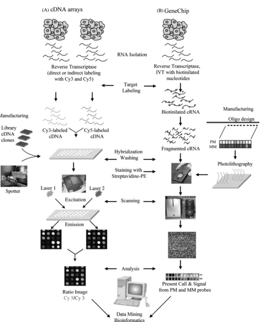
Microarray Today exists a large variety of microarrays technologies to measure dierent kinds of biological data like gene expression, protein abundance, protein binding or genomic aberrations. Their advantage compared to other methods is, that they measure not only one gene or protein at a time, but thousands. Therefore, microarray data are snapshots of an entire proteome or transcriptome within a sample at a certain time point. In this work we focus mainly on gene expression microarray data, which was also the rst application of this technology. There are two primary types of gene expression microarrays: (i) The cDNA microarray which was invented by the Pat Brown laboratory in 1995 (Schena et al., 1995) and (ii) the high-density oligonucleotide array invented by Aymetrix in 1996 (Lockhart et al., 1996).

The basic concept of any gene expression microarray experiment is to extract mRNA from a tissue and reverse transcribe it into cDNA. As a prerequisite for measuring, cDNA is amplied in a way that the relative molecular abundances of dierent mRNAs are preserved. The cDNA is then labeled with a uorescent dye and used as a target to bind to complementary DNA sequences. The targets are detected by single-stranded cDNA or oligonucleotide probes that are attached as xed spots on a support surface like a glass slide. The abundance of a particular mRNA can be measured indirectly by quantifying the uorescence intensity of the corresponding probe spot. A quantication of the measured mRNA abundance can be done by comparing the spot intensities of a sample to the intensities of a control experiment. This quantication is not absolute but relative to the control. Figure 1.1 illustrates the generation and application of cDNA and high-density oligonucleotide arrays.

Until today microarray technologies have been developed to be routine high throughput methods that have been proven to be a valuable tool of modern molec-ular biology. Their versatility is highly responsible for their success. They can be employed to detect dierentially expressed genes between samples of dierent bi-ological origin (Chee et al., 1996), or to identify a set of genes that discriminates between dierent types of samples for diagnosis or prognosis (van 't Veer et al., 2002). They can also be used to dene novel subgroups within a certain sample population (Alizadeh et al., 2000). Other microarray technologies can be used for polymorphism analysis (Wang et al., 1998), sequencing (Pease et al., 1994) and

(29)

de-Figure 1.1: Comparison of the production and hybridization steps in (A) cDNA and (B) high density oligonucleotide arrays.

tection of protein DNA interactions (Ren et al., 2000). Data analyzed in this thesis primarily originates from gene expression microarray experiments. In chapter 4 we use additional data from ChIP-on-chip experiments.

qPCR (quantitative Polymerase Chain Reaction) Polymerase chain reaction

is a technique for DNA amplication. In theory, PCR can produce an arbitrary number of copies out of a single DNA segment. It was developed in the 1980s by the American biochemist Kary Mullis, who was rewarded with the Nobel Price for

(30)

chemistry in 1993.

The PCR process runs in cycles, which each consist of three steps, namely de-naturation, primer annealing and elongation. In each cycle the amount of DNA molecules is doubled. In the denaturation step the two DNA strains are separated by heating. Then follows the annealing step in which the temperature is lowered to allow the primer sequences to bind to the single stranded DNA. In the elongation step the DNA polymerase replicates the second strain of each single stranded DNA molecule. It is possible to amplify only specic DNA segments by using only primers that ank the targeted sequence. Hence PCR allows both, the amplication of the whole genome or specic DNA segments. PCR can also be used to amplify RNA. To do so RNA molecules have to be transcribed into cDNA molecules before the amplication process is started. This transformation is called reverse transcription. Apart from amplication PCR can also be used to quantify the initial amount of targeted transcript. This method is called quantitative PCR (qPCR). For the quantication uorescent dyes are used that are build into the replicated sequence during the elongation step. With each cycle the dye intensity increases as the num-ber of transcript copies increase. The numnum-ber of cycles is counted until a specic intensity threshold is reached. This number is compared to a reference PCR using a target sequence with known abundance (Wang et al., 1989). This technique can be used to detect chromosomal aberrations like copy number changes or to measure gene expression if qPCR was done on reverse transcribed cDNA.

Apart from being an integral part of experimental protocols generating microarray data, PCR was used to validate results from microarray gene expression analysis in chapter 4.

ChIP-on-chip ChIP-on-chip combines chromatin immunoprecipitation (ChIP)

with the microarray technology (chip). The ChIP technique isolates and identies DNA sequences that were be bound by specic DNA binding proteins, for example transcription factors (Ren et al., 2000). In principal, DNA is cross linked with the protein of interest and sheared. Then the DNA fragments with a bound protein are separated from all other DNA fragments using antibodies specic to the protein of interest. Depending on the specic method these antibodies are attached to a solid surface or have a magnetic bead that allows the xation of the protein-DNA complexes, such that the other DNA fragments can be washed away. The bound DNA segments are then separated from the protein of interest and puried. After

(31)

amplication the DNA segments are denatured into single stranded DNA fragments. These are labeled with a uorescent dye. The labeled fragments are then hybridized to a DNA microarray. As each spot of the microarray represents a specic location in the genome one can identify the DNA binding positions by identifying spots with high uorescence intensities. In chapter 4 we use data from ChIP-on-chip experiments to identify gene clusters that are targets of the transcription factor BCL6.

(32)

(33)

Chapter 2 Statistical Context

2.1 Machine Learning

Notation This thesis deals with gene expression microarray data. Here we give the notation that will be used throughout the thesis. We will denote data sets consisting of n samples and p genes by a matrix X ∈ Rp×n. Each row xi· of X

contains the expression of a single gene across all samples, while each column x_·j

contains the expression prole of a single sample. Denoting a gene by an index letter, like any gene g, is equivalent to xg·. If we work on more that one data set

simultaneously, we will introduce notional conventions when needed. In some cases additional information is available that assigns samples into groups or classes. We will call this information labels and store them in a vector Y with yj ∈ [1, . . . , k]

and j = 1, . . . , n, where k is the number of classes.

Un-, Semi- & Supervised Learning Machine learning problems are categorized into three dierent groups, namely un-, semi- and supervised problems. Unsuper-vised learning seeks to determine how data is structured. Well known examples of unsupervised methods are clustering and density estimation. Cluster algorithms aim to separate the data objects into a given number of groups. Density estimation analyzes how the data objects are distributed in the data space.

In contrast, supervised learning problems arise from data sets that consist of inputs and outputs. Inputs could be expression proles x_·j of patient samples and

the corresponding outputs could be class labels yj. Supervised methods aim to

predict the output from the inputs. Applications of supervised learning are for 13

(34)

example classication and regression methods.

Semi-supervised problems are halfway between supervised and unsupervised prob-lems. Here the output information is given only for a part of the inputs, meaning that labels are only available for some expression proles. Similar to supervised methods the goal is to predict the outputs of all inputs. Semi-supervised learning methods extend supervised approaches by incorporating structural or distribution properties learned from the unlabeled inputs.

2.1.1 Classication

Classication is one of the major applications of supervised learning. Given a gene expression data set X with corresponding class labels Y, we denote a classier or

prediction model that has been estimated from training data as fclass(X). For a

certain expression prolex_·j the predicted label is denoted as fclass(x·j). Dierences

between fclass(x·j) and the corresponding label yj are called errors. The number of

errors made by a classier is measured by a loss function

L(yj, fclass(x·j)) =    1 if yj =fclass(x·j) 0 if yj 6=fclass(x·j) (2.1) One distinguishes between two types of errors, the training and the test error. The training error is the average loss over the training samples

err = 1 n n X j=1 L(yj, fclass(x·j)). (2.2)

However, to assess the quality of a classier one uses the test error, which is estimated by the average loss over an independent test data set X0 containing n0

samples and known class labelsY0 Err = 1 n0 n0 X j=1 L(y_j0, fclass(x0_·j)). (2.3)

In the next part follows a detailed explanation of the nearest shrunken centroids (NSC) classication algorithm.

Nearest Shrunken Centroids The NSC method was proposed by Tibshirani

et al. (2002) and is designed for the analysis of microarray expression data. In this context the task is to classify and predict the diagnostic category of a sample

(35)

based on its gene expression prole. This classication problem is challenging since one is faced with a large number of genes from which to predict classes for a small number of samples. It is important to identify the genes that contribute most to the classication, so that non-contributing genes can be discarded.

Given a gene expression data set X and a vector of corresponding class labels Y ∈1,2, . . . , K, letCk be a vector of indices of the nk samples belonging to class k.

The centroidx¯_·k of a classk is dened as the average expression per gene across all

samples of that class: x¯ik = P

j∈Ckxij/nk. Similar, the overall centroid is dened as the average expression per gene across all samples x¯i =

Pn

j=1xij/n. In order

to identify genes that contribute most to the classication the class centroids are shrunken stepwise towards the overall centroid. This is done by comparing the centroid of each class k to the overall centroid. We dene a dierence dik for each

gene as dik = ¯ xik−x¯i mk·(si+s0) (2.4) where each gene is standardized by the pooled within-class standard deviation

s2_i = 1 n−K X k X j∈Ck (xij −x¯ik)2 (2.5) and mk = p

1/nk+ 1/n, so that mk·si is equal to the estimated standard error of

the numerator indik. The positive constants0guards against largedik values arising

from genes with low overall variance. Shrinkage is done by reducing the values of

dik stepwise towards zero. This process is tuned by a parameter∆

d0_ik =sign(dik)(|dik| −∆)+, (2.6)

where sign(x) equals 1 or −1 if x is positive or negative and (|dik| −∆)+ denotes

the maximum of |dik| −∆ and zero. Genes are discarded if d0ik becomes zero. A

shrunken class centroid x¯0_ik can then be dened by rewriting equation 2.4 as ¯

x0_ik = ¯xi+mk(si+s0)d0ik . (2.7)

A samplex_·j is classied by determining the closest shrunken class centroid. The

distance between a class centroid and a sample is measured by the discriminant score δk(x·j) = p X i=1 (xij −x¯0ik)2 (si+s0)2 − 2 logπk (2.8)

(36)

where πk is the prior probability of class k, that is dened as the overall frequency

of class k in the population, hence PK_k=1πk = 1. Usually πk is set to nk/n. The

prediction model is then dened as

fclass(x·j,∆) =r where δr(x·j) = min

k δk(x·j). (2.9)

The result of the NSC classier depends on the chosen shrinkage parameter ∆. We chose∆so that the test error is minimized by employing a cross validation procedure as described below.

Cross Validation Cross validation (CV) is a method widely used for model

assessment and selection. Here we will consider CV in the context of classication. CV is one of the simplest ways for estimating the test error of a classier or prediction model. Given a gene expression data setX with corresponding class labelsY and a

prediction modelfclass(X) one can assess the performance of the fclass(X)using an

independent test set. Unfortunately, this is often not possible since data is scarce. To circumvent this problem CV uses one part of the available data to train the model and another part to test it. The data is split into K subsets (or folds) of

equal size (K-fold CV). Each of the K subsets is predicted by a model trained on

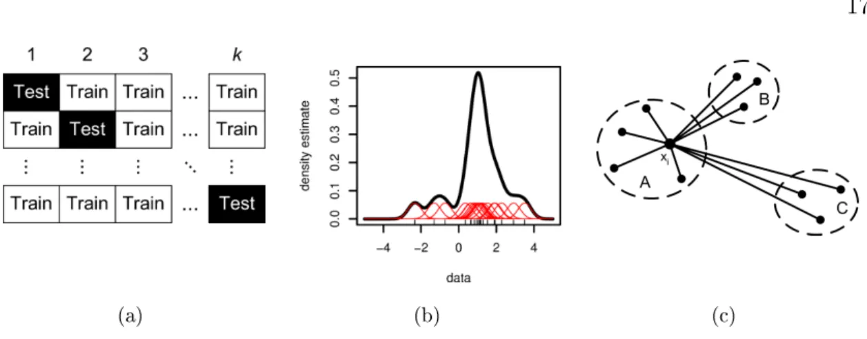
the otherK−1sets. Figure 2.1(a) illustrates the arrangement of a data set into K

subsets and the K training / prediction runs. The test error is then calculated by

combining the errors in theK predicted subsets. The CV estimate of the test error

is dened as ErrCV = 1 n n X j=1 L(yj, f− k(j) class (x·j)) (2.10)

wheref_class−k(j)(x_·j)is the prediction model trained without the subsetk that contains

samplej. Common choices ofK are 5 or 10. IfK equals n one speaks of

leave-one-out cross validation. In this work 10-fold CV was used if not stated otherwise. If the training procedure of a prediction model depends on a tuning parameter∆, one can use CV to determine the optimal choice of∆. In case of the NSC classier ∆is the amount of shrinkage. We index the set of models by fclass(x·j,∆). For each

∆the CV error is dened as

ErrCV(∆) = 1 n n X j=1 L(yj, f− k(j) class (x·j,∆)) . (2.11)

ErrCV is an estimate of the test error as a function of ∆. The optimal choice of

(37)

(a) (b) (c)

Figure 2.1: (a) Cross validation scheme: Each row represents an individual classi-cation run, while the columns indicate the division of the samples into k sub sets.

During each run, the classier is learned on the training set and used to predict the test set. (b) Density estimation for a small data set consisting of 20 elements. The density estimate at each point (black line) is the average contribution from each of the Gaussian kernels (red lines). The kernels were scaled down by the factor of 20 to t in the graph. The data points are indicated by vertical bars at the bottom. (c) Arrangement of elements involved to calculate the silhouettes(i) of element xi

belonging to cluster A. B is the nearest neighborhood cluster of xi and C is an

other, more distant cluster.

model is then fclass(X,∆0). In case of the NSC classier ∆0 is determined by trying

dierent choices of ∆.

2.1.2 Kernel Density Estimation

Given the gene expression data set X we assume that the p genes xi· are sampled

independently from an unknown distribution. Kernel density estimation (KDE) is an unsupervised learning procedure that aims to estimate the probability density functionfdens(x)from the given data set X, for anyx∈Rp. A local estimate of the

probability density atx has the form

ˆ

fdens(x) =

#{xi·∈ N(x)}

p σ (2.12)

whereN(x)is a small metric neighborhood around xof width σ and#{. . .}counts

the number of genes inN(x). This function tends to be rough, since genes can either be inside or outside a neighborhoodN(x). A smoother function can be achieved by using the Parzen estimate, which weights the counting as a function of distance to

(38)

xi· ˆ fdens(x) = 1 p σ p X l=1 Kσ(xl·, x) (2.13)

where Kσ(xl·, x) is a function with bandwidth σ that gives decreasing weights to

genesxl· as the distance to xincreases. Kσ can be seen as a function that measures

the similarity between two genes. The closer the genes are, the higher is their similarity. Such functions are also called kernels. The Gaussian kernel is a popular choice forKσ. Assuming mean zero and standard deviation σ equation 2.13 has the

form ˆ fdens(x) = 1 p√2σ2_π p X l=1 exp −||xl·−x||2 2σ2 . (2.14)

An example for density estimation using a Gaussian kernel is shown in Figure 2.1(b).

The bandwidth σ of the kernel is a parameter that has a strong inuence on

the resulting density estimate. Small σ lead to under-smoothing resulting in

spu-rious data artifacts. On the other hand large values lead to over-smoothing which obscures much of the underlying data structure. A popular measure to assess the accuracy of the estimated density function is the mean integrated squared error (MISE) suggested by Rosenblatt (1971):

MISE=E|fdens(x)−fˆdens(x, σ)|2 =

1 p p X i=1 fdens(xi·)−fˆdens(xi·, σ) 2 (2.15) where_fˆ_dens₍_{x, σ}₎_{is a set of estimated density functions indexed by}_σ_{. However, this} measure assumes that the true density is known which is usually not true. This led to numerous data driven bandwidth selection methods of which the cross validation and plug-in methods suggested by Rudemo (1982), Bowman (1984), Park and Marron (1990) and Sheather and Jones (1991) are most popular and well established for low dimensional data. Unfortunately, when working with high dimensional data like gene expression measurements such methods are not applicable as they are computational complex and time intensive. A careful selection by hand is more practicable.

2.1.3 Clustering

Clustering can be dened as the segmentation of data based on a (dis-) similarity measure. This segmentation results in a grouping of data objects into subsets or 'clusters', such that data objects in the same cluster are more similar than data

(39)

objects in dierent clusters. Importantly, each object needs to be assigned to exactly one cluster. Additionally, some cluster methods arrange the clusters in a natural hierarchy. This is done by successively grouping the clusters themselves so that at each level of hierarchy clusters within the same group are more similar as those in dierent groups.

There exist dierent types of cluster algorithms. A very popular type is combi-natorial clustering. Such algorithms directly assign data objects to clusters without referring to probabilistic data models. Given a gene expression data setX, the data

objects that are to be clustered can be genes as well as samples. We dene the dis-similarities between each pair of data objects, here samples, by a distance function

d(x_·j, x·l). The pairwise distances are stored in a symmetric matrix D. A popular

distance measure is the Euclidean distance

Djl=d(x·j, x·l) = v u u tXp i=1 (xij −xil)2 . (2.16)

Clustering aims to separate the samples intoK clustersCi, withi= 1, . . . , K where

each cluster Ci stores the sample indices of cluster i, so that samples within the

same cluster are more similar than samples within dierent clusters. The within cluster distances, can be measured by a loss function

Dwithin= K X k=1 X j∈Ck X l∈Ck Djl. (2.17)

A clustering that minimizes Dwithin will be optimal, as it automatically maximizes

the between cluster distances

Dbetween= K X k=1 X j∈Ck X l /∈Ck Djl (2.18) since

Dtotal =Dwithin+Dbetween= n X j=1 n X l=1 Djl . (2.19)

The optimal clustering can be found by enumerating all possible partitions into

K clusters. However, this is only feasible for small data sets as the number of

combinations growth rapidly with increasing data size. To circumvent this problem practical combinatorial cluster algorithms try to examine only a small fraction of all possible partitions. The goal is to identify a small subset that is likely to contain the

(40)

optimal one, or at least a good suboptimal partition. The algorithm that was used in the thesis is partitioning around medoids that is described in the next section.

Partitioning around Medoids The partitioning around medoids (PAM)

algo-rithm was proposed by Kaufman and Rousseeuw (1990). Given a gene expression

data set X and the number of clusters K, the method aims to nd a set M of K

representative data objects (medoids). This set denes a clustering by dividing the data objects intoK groups, so that each object belongs to its nearest medoid. The

set of medoids is chosen such that the sum of distances of each data object to its closest medoid is minimized. The PAM algorithm consists of two phases, the build phase and the swap phase. During the build phase K medoids are added

consecu-tively to the set of medoidsM, while in the swap phase this set is improved. In the

following we assume that we cluster the samples x_·j of the gene expression data set

X.

The build phase is initialized by selecting the rst medoidm1. This is the sample

that minimizes the sum of dissimilarities between itself and all other samples. Hence,

m1 is the sample that is most centrally located in the data set. All other medoids

mi with i= 2, . . . , k are chosen iteratively by maximizing the loss function

Lbuild(x·j) = n X l=1 min m∈M[d(m, x·l)]−d(x·j, x·l) (2.20) where minm∈M[d(m, x·l)] is the minimal distance between a sample x·l and the

al-ready chosen medoidsm, andd(x_·j, x·l)is the distance between two samples x·j and

x_·l. Lbuild(x·j)is the number, by that the sum of distances between samples and their

closest medoids would be reduced if x_·j was added to the set of medoids. In each

iteration step Lbuild is calculated for all samples x·j and the sample that maximizes

Lbuildis added to the set of medoidsM. This procedure is repeated untilK medoids

are found.

In the swap phase the algorithm aims to improve the set of medoids M and

therefore also the clustering implied byM. This is done by iteratively searching the

pair of objects (mi, x·j) that if swapped, reduces sum of distances between samples

and their closest medoid most. A swap (mi, x·j)means thatmi is removed from and

x_·j is added to the set of medoids. We denote the new set of medoids generated by

(41)

between samples and their nearest medoids induced by the swap (mi, x·j). Lswap(mi, x·j) = n X l=1 min m0∈M0d(m 0_{, x} ·l)− n X l=1 min m∈Md(m, x·l) (2.21)

Details of an ecient implementation of this loss function can be found in Kaufman and Rousseeuw (1990). Lswap(mi, x·j)can take negative or positive values depending

on whether the swap was benecial or not. Negative values indicate benecial swaps as sum of minimal distances between samples and their closest medoids is reduced. The optimal swap is the one that minimizes Lswap. This iteration is repeated until

no benecial swap remains.

Following this heuristic procedure the resulting partition will not necessarily be the global optimum with minimal sum of the within cluster distances Dwithin (see

equation 2.17) but a good approximation. The number of clusters K in which the

data set is separated is a parameter and has to be specied. To select the optimal

K a measure is needed that assesses the quality of a given clustering. However, sum

of distances between data objects and their closest medoid, which is a result of the PAM procedure, orDwithin can not be used, as it decreases naturally with increasing

K. Because of this an external cluster validation score has to be used. In this thesis

the silhouette score is employed.

Silhouettes Various methods are available that segment a given data set into a set of K clusters, like K−means, K−medians or the PAM algorithm that is used

throughout this thesis. All of these methods result in a set of clusters, where each cluster contains a certain number of data objects. However, it remains unclear if these clusters reect a structure that is truly present in the data, or if the data was just segmented into some articial groups. In the end, cluster methods always segment the data intoKgroups, regardless whether this is supplied by data structure

or not. A method is needed that assess the quality of a given clustering. Dierent methods have been proposed in the literature and some of them were compared by Smolkin and Ghosh (2003). The various methods mainly dier in their denition of cluster quality. In this thesis we employ the method proposed by Rousseeuw (1987) and calculate silhouettes to assess cluster quality. Using silhouettes, clusters are of high quality if data objects within the same cluster have low dissimilarities or distances compared elements in dierent clusters. This denition is particularly justied with respect to the PAM algorithm, since PAM aims to segment data, such that the within cluster distances are minimized.

(42)

Given a gene expression data set X, a matrix of pairwise distances D and a set

of clusters, then the silhouettesi of a sample x·i belonging to clusterA is dened as

si = bi−ai max (ai, bi) (2.22) where ai = 1 NA X x_·j∈A d(x_·i, x·j) (2.23)

is the average distance of x_·i to all other samples of A, with NA being the number

of samples in A, and bi = min C6=A 1 NC X x_·j∈C d(x_·i, x·j) (2.24)

is the minimal average distance ofx_·i and all samples of any clusterC dierent from

A. We denote the cluster for which the minimum bi is achieved as neighborB ofxi.

Figure 2.1(c) illustrates the arrangement of the clusters A, B and C. If a cluster

contains only one elementsi = 0.

From the denition above follows that

−1≤si ≤1 (2.25)

for each sample x_·i. Large si, that are close to 1, imply that the within cluster

dissimilarityai is much smaller than any between cluster dissimilaritybi. Hence,x·i

can be considered as well clustered. Vice versa small values of si mean that ai is

much larger than bi, so that on average x·i is situated much closer to its neighbor

cluster B than to A. Therefore it seems to be more natural to assign x_·i to its

neighborB, meaning thatx_·i has been misclassied. If si is about zero, thenai and

bi are approximately equal and it is not clear if x·i belongs to cluster A or B.

The silhouettes dene a measure how well each sample x_·i matches the given

clustering. To assess the quality of a given clustering we calculate the average silhouette ¯ s = N X i=1 si . (2.26)

One can compare a set of dierent clusterings by comparing their average silhouettes. The clustering that obtains the maximal average silhouette ts best to the data structure. Following this, the parameterK of the PAM algorithm can be tuned by

(43)

2.1.4 Dierential Gene Expression

Given a gene expression data setX consisting of two dierent types of samples, for

example tissue biopsies of healthy (group A) and diseased patients (group B), then

dierentially gene expression analysis describes a set of methods that answer the question whether the expression levels of a gene xi· diers systematically between

the two groups. This dierence is usually dened as the dierence between the mean expression within groupA and B.

While the details may dier depending on the method, the general concept is to assume that a gene is not dierentially expressed between the groups and then test this null-hypothesis using an appropriate statistical test. Formally we dene the null-hypothesis H0 for each gene g:

H0 :The gene is not dierentially expressed.

If H0 is rejected by the test, then g is considered to be dierentially expressed

between the two classes. The test that is most commonly used is Student's t-test, which combines the mean dierence between the groups with the variance within the groups. Assuming equal variance in both groups thet-score is dened for each

gene ias: ti = ¯ xiB−x¯iA si , (2.27) wherexiA= _n1 A P

j∈Axij, the value ofxiB is dened similar, andnA andnB are the

number of samples in the groups. The pooled standard deviation si is dened as

s2_i = 1/nA+ 1/nB nA+nB−2 X k={A,B} X j∈k (xij−x¯ik)2 . (2.28)

A look-up ofti in thet-distribution delivers the probability (p-value) of obtaining a

test statistic with absolute value of at least|ti| by chance. The p-value is then used

to decide whetherH0 is rejected or not. If the p-value is below a certain signicance

threshold, usually 0.05, H0 is rejected and a gene is said to be dierentially

ex-pressed. However, in the context of gene expression analysis this raw p-value can be misleading since several thousand genes are tested simultaneously. A large number of simultaneous tests leads to an unnatural high rejection rate ofH0. The

percent-age of genes equal to the selected signicance threshold will be rejectH0 by chance.

This observation is called multiple-testing problem. Several statistical methods have been developed to correct the raw p-values for multiple testing. Throughout this

(44)

thesis the method proposed by Benjamini and Hochberg (1995) was used. The re-sulting adjusted p-values (Padj) reect the false discovery rate (FDR), which is the

(45)

Part II

Genomic Data Integration

(46)

(47)

This part focusses on genomic data integration in the context of gene expression experiments using microarray technology.

We begin in chapter 3 with reviewing the literature on data integration methods and concepts. Since data integration is a broad eld with application ranging across various methods, data sources and types, we will focus on literature that is closely connected to the topic of this thesis.

We continue in chapter 4 with the introduction of a novel data integration method for the simultaneous analysis of clinical microarray gene expression proles and ex-perimental data.

(48)

(49)

Chapter 3 A review on genomic data

integration

In recent years, the number of available molecular biological methods has immensely increased. Today, modern technologies allow an almost complete characterization of biologic samples on the cellular level. Complementary properties include determi-nation of genotypes using PCR or DNA sequencing and investigation of the DNA methylation status as well as transcriptome, proteome and metabolome snapshots. Further, chromatin immunoprecipitation assay like ChIP-seq allow proteDNA in-teraction studies. Additionally, protein-protein inin-teraction and protein localization screens are available that allow deeper insights into the biomolecular interplay within cells. Many more methods exist, but not all can be mentioned here. However, even if partly complementary, each proling method sheds dierent light on the function-ing and malfunctionfunction-ing of cells. Their joint full potential can only be realized when dierent sources are combined. Furthermore, research is done on and with dierent species and model organisms. New challenges arise in cross-species analyzes since genomes and biomolecular interplay are similar but not identical. However, the value of model organism in biological and medical research has been shown in many applications. The development of new drugs and therapies always involves animal tests and cell culture experiments. Thus, integrating data from dierent sources is an important part of modern biomedical research. An important aspect of data integration is the development of tailored statistical methods that are able to lever-age knowledge contained within a diverse range of data sources and at the same time, being able to provide evidence to answer the types of question being posed

(50)

by the research community as a whole. While the concept of statistical data inte-gration is self evident, its realization in genomics is challenging. Obstacles include the heterogeneity of experimental setups, study designs, proling platforms, sample handling, and data management. Furthermore, missing meta-data and insucient documentation of heuristic and complex multistep analysis procedures complicate the endeavor.

According to Pavlidis et al. (2002) data integration methods can be divided into three dierent types depending on the analysis step at which the integration is done. They distinguish between early, intermediate and late integration. Early integra-tion takes place on the level of input data by simply unifying dierent data sets to a single one. The analysis is then done by applying standard methods to the unied data. This approach demands that the dierent data sets are of similar type or have a common feature space and scale. For example one can combine dierent gene expression data sets if the same platform was used, or if the platforms dier the measured genes overlap. In contrast late integration takes place on the level of analysis results. Here data from dierent sources is analyzed individually and the nal statistical results are combined. Following this approach heterogeneity in data type and analysis procedure can be overcome. Intermediate integration describes the simultaneous analysis of several data sources. The integration step is implemented within the analysis procedure. Such methods are more complex than the analysis of a single source and are often tailored towards a specic problem. However, si-multaneous analysis allows a more exible manipulation of the integration process. In their work Pavlidis et al. (2002) shows that the intermediate integration is often superior to early and late approaches but requires sophisticated weighting of each data type.

In biomedical research late data integration enjoys great popularity as it allows the combination of heterogeneous data types. The prerequisite for late data inte-gration is converting data from dierent sources into a common format. One format that is widely used are gene sets or ranked lists of genes as they can represent a variety of dierent informations like expression dierences, binding anities and molecular functions or processes. Dierent methods have been proposed by Beiss-barth and Speed (2004), Subramanian et al. (2005) and Lottaz et al. (2006) tailored towards specic problem settings. In order to gain biological insights from a gene list it is necessary to analyze the functional annotations of all genes in the list.

(51)

These annotations were experimentally determined and validated. Each annotation describes properties of a set of genes or their products. Each gene may have several annotations. Beissbarth and Speed (2004) identify annotations that are statistically signicant within a given gene list by comparing the annotation present in the list with a control set of genes. While the gene list of interest is usually a handful of genes showing strongest response to the experiment, the control set can be a database of annotated genes or all annotated genes represented on a microarray. Annotations signicantly over represented in the gene list compared to the control set are de-scriptive for the list and experiment. A major drawback of this over-representation analysis is that the gene list was usually produced by a single-gene analysis like dierential expression analysis. This may miss important eects on pathways, since cellular processes often aect sets of genes. For instance, a relative small increase in the expression of all genes encoding members of a metabolic pathway may dramat-ically inuence the biologic processes regulated by that pathway more dramatdramat-ically than a high increase of expression in a single gene. To overcome this problem Sub-ramanian et al. (2005) suggest to measure the enrichment of gene sets in ranked lists that include all genes measured in the experiment. Consequently they call their approach gene set enrichment analysis (GSEA). Given multiple ranked gene lists Lottaz et al. (2006) detects considerable overlaps among the top-ranking genes. Gene sets conserved across ranked lists emerging from dierent experiments (dier-ent species) may hold information about conserved biological processes.

Integration on the level of gene lists avoids the need for joint quantitive data models that describe the dependencies between individual proles.

A quantitative early integration approach is the concatenation of feature vectors from dierent platforms in the context of classication problems. If several types of high dimensional readouts are available for the same group of samples, predic-tive signatures can be constructed by combining selected features across all data types thus exploring potential complementary information. Somewhat surprisingly, several authors observed only marginal improvements in classication accuracy re-sulting from early data integration. Boulesteix et al. (2008) report on several cancer types where the integration of microarray data with standard clinical predictors, like age or sex is not benecial. The authors give two possible explanations for this observation. First, the microarray data might be simply not relevant for the classi-cation problem and therefore not improve any classier nor be able to achieve high

(52)

accuracy alone. Second, the microarray is relevant for the prediction problem, but redundant or weaker than the already available clinical parameters. In this scenario classication on the microarray data alone would have good performance. However, such redundancy does not imply a causal relationship between clinical parameters and gene expression. Edén et al. (2004) already observed that 'good old' clinical markers have similar prognostic power as microarray gene expression data. Similar results were reported by Lu et al. (2005) in the context of prediction protein-protein interactions from genomic features like mRNA co-expression, functional similarity or phylogenetic proles. The authors extended the original feature list of Jansen et al. (2003) by additional features. However, even if those new features showed high univariate prediction strength and were largely conditionally independent no improvement of classier performance was observed. Lu et al. (2005) reason, that integrating a few good features already approaches the maximal predictive power, or limit, of current genomic data integration.

Both examples show that simply piling up more and more data sources will not nec-essarily lead an improvement of existing analysis results or new biological insights.

In contrast to integrating several data sources within the same sample population data integration methods can also be used to aggregate information across dierent sample populations. A prominent example for this application is the integration of clinical and experimental sample population in the eld of gene expression analysis. In this context Bild et al. (2006) combined expression data generated experimen-tally by overexpression of active oncogenes in quiescent primary human mammary epithelial cells (HMECs) with tumor samples of various carcinomas. Oncogene spe-cic gene signatures were identied by comparing the oncogene transfected HMECs with a control group employing a Bayesian binary regression procedure proposed by West et al. (2001). These signatures were then used to predict oncogenic activation probabilities of the tumor samples by applying the regression model. The authors showed that combinations of activation probabilities of dierent oncogenes can pre-dict outcome and treatment eciency of the cancer samples. This analysis strategy is sequential in that predictive gene sets are identied and combined to predictive signatures in the HMECs only. In a second independent integration step they are applied to clinical data. Note that this procedure is fully supervised as signatures are not aected by properties of the clinical data.

(53)

The authors start their analysis on the clinical data. For each gene they generate a gene set by selecting all genes that exceed user a dened correlation threshold with the respective gene. Those gene sets are then tested for joint dierential expression between the dierent experimental conditions within the HMECs. The authors re-ject all gene sets that do exceed a certain threshold of signicance. Although the authors ensure correlation between genes within the tumor samples and joint dier-ential expression in the HMECs, the HMECs do not inuence the formation of gene clusters.

The rst analysis approach combining both data sets from the onset was described by Bentink et al. (2008). This new approach is based on an unsupervised class discovery procedure proposed by von Heydebreck et al. (2001) that searches for bi-partitions within a gene expression data. Bentink et al. (2008) rened this method to meet a semi-supervised scenario in which the tumor data is the unlabeled and the HMECs the labeled data. This semi-supervised approach allows the authors to nd classication of tumor samples based on coherently expressed genes, that simultaneously separate experimental conditions.

In the owing chapter of this thesis we will complement and extend the approach of Bentink et al. (2008). We will develop a novel data integration strategy named guided clustering that combines experimental and clinical high throughput data of possibly dierent genomic data types. Guided clustering is tailored to analysis scenarios, where the construction of a diagnostic signature is not driven by class labels on the clinical data, for instance disease types or clinical outcomes, but by a biological focus for example the activity of a transcription factor or an entire pathway. The biological focus of the signature is established by a complementing experimental study on model organisms like cell lines or mice. Examples for those experimental studies are cell line perturbation experiments as performed by Bild et al. (2006) or proling of CpG methylation status as done by Gebhard et al. (2006). Guided clustering uses a density estimation approach to identify sets of genes that show strong response to the experimental condition while at the same time display coherent expression across the clinical data set. In contrast to the semi-supervised approach of Bentink et al. (2008) guided clustering operates fully unsupervised. Nevertheless the feature selection procedure that drives ordering of patient samples is guided by the complementing experimental data. Furthermore guided clustering extends the framework of previous methods in that it allows the

(54)

integration of data from dierent genomic platforms. Instead of separating clinical samples into classes our approach provides quantitative predictions of experimental conditions like pathway activation.

In principal, guided clustering can be applied to any data integration problem that links a sample clustering problem to a feature selection problem driven by a second data set. In the next chapter we will introduce our method in detail and compare its performance with other approaches. Further, we will report on two exemplary applications: (i) The prediction of transcription factor activity in clinical samples guided by a chromatin immunoprecipitation experiment and (ii) the prediction of pathway activity guided by cell culture perturbation experiments.

(55)

Chapter 4 Guided Clustering

4.1 Problem Setting

Gene expression analysis of cancer biopsies has been subject of intensive research in recent years. A detailed characterization of patient samples is vital for diagnosis and treatment. There exists a multitude of techniques that allow determination of dierent characteristics, for example staining of protein markers, comparative ge-nomic hybridization (CGH) to determine gege-nomic aberrations and other microarray technologies that create snapshots of the transcriptome or proteome. In practice not every technique can be applied to every sample since modern biomolecular meth-ods are often cost intensive. However, due to the interaction between all cellular components and processes malfunctions can be observed with several measurements. For example genomic aberrations can be directly detected by CGH, but they will also eect the transcriptome and proteome, so that they can often be detected by microarrays too as shown by Mullighan et al. (2009). Gene expression microarrays have been proven to be a valuable tool to distinguish between cancer types and sub-types (Golub et al. (1999), Alizadeh et al. (1999), Bea et al. (2005) and Dave et al. (2006)) and also dened new disease subtypes (Alizadeh et al. (2000) and Sotiriou et al. (2003)). This renement of diagnosis can greatly improve the treatment ef-ciency of patients, since dierent cancer subtypes show dierent drug resistances (Staunton et al., 2001). Obviously, it would be extremely helpful, if one could specif-ically design experiments to search for subgroups of interest. Experiments necessary to dene such groups are for example knock-down through RNAi, the transfection of constitutively active forms of genes, or application of drugs. However, such

(56)

periments can not be conducted directly on the patient population. This lead to the approach to perform experiments of interest on model organisms, observe the responses and search similar patterns in patient data. For example, gene expression proles of a model organism can measure the gene-wise response to certain pertur-bations. The knowledge of those responses have two mayor benets: (i) It may guide to potentially interesting sets of correlated genes, since they react to perturbation, and (ii) delivers a possible explanation for the coherent expression among patient samples. This setting leads to the data integration problem of identifying sets of genes that are coherently expressed across patient samples and showing perturba-tion response in a model organism. In the following we will refer to the perturbaperturba-tion experiment as the guiding data.

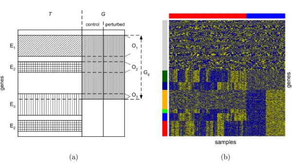
LetTij be a matrix of tumor expression proles and Gij the guiding data, where

rowsidenotes genes while columnsj denotes samples. For simplicity, we assume that

the same proling platform is used and hence the same genes are monitored in both data sets. The guiding data setGconsists of two types of samples: Those which were

subject to perturbation and the corresponding unperturbed control group. Since we know which proles were experimentally perturbed and which not the guiding data set is labeled. The labels are stored in a binary vector Y, where a perturbed

prole is indicated by a one and a control sample by a zero. Like experimental perturbations, somatic mutations in cancers can eect gene regulation and leave similar traces in expression proles. Hence, we assume that the eect modeled by the perturbation experiment is also present within the tumors samples and varies across T due to dierent somatic mutations. However, a priori it is unknown in

which tumor samples a perturbation eect is present and to what extend. Thus the data setT is unlabeled.

In the following sections we describe an algorithm called guided clustering that aims to detect and quantify the presence of a perturbation within tumor data sam-ples by identifying sets of genes that are coherently expressed within T and show

strong perturbation response in G. The ndings of this work are published in the

Genomic data integration & gene expression analysis of single cells

Genomic Data Integration

&

Gene Expression Analysis of Single Cells

Dissertation zur Erlangung

des Doktorgrades der Naturwissenschaften (Dr. rer. nat.)

der Fakultät für Biologie und Vorklinische Medizin

der Universität Regensburg

vorgelegt von

Herrn Matthias Maneck M.Sc.

aus

Berlin

im Jahr 2011

Die Arbeit wurde angeleitet von:

1. Betreuer: Prof. Dr. Wolfram Gronwald

2. Betreuer: Prof. Dr. Rainer Spang

Unterschrift:

Contents

I Introduction

1

II Genomic Data Integration

25

III Analysis of Single Cells

63

IV Appendix

103

List of Figures

List of Tables

Abbreviations and Notation

Preface

Acknowledgement

Figures

Part I

Introduction

Chapter 1

Biological Content

1.1 Molecular Biology

1.2 Measuring Techniques

Chapter 2

Statistical Context

2.1 Machine Learning

2.1.1 Classication

2.1.2 Kernel Density Estimation

2.1.3 Clustering

2.1.4 Dierential Gene Expression

Part II

Genomic Data Integration

Chapter 3

A review on genomic data

integration

Chapter 4

Guided Clustering

4.1 Problem Setting