Journal of Statistical Software
August 2017, Volume 79, Issue 10. doi: 10.18637/jss.v079.i10Simulation of Synthetic Complex Data:
The
R
Package
simPop
Matthias Templ Zurich University of Applied Sciences Bernhard Meindl Statistics Austria Alexander Kowarik Statistics Austria Olivier Dupriez World Bank Abstract
The production of synthetic datasets has been proposed as a statistical disclosure control solution to generate public use files out of protected data, and as a tool to cre-ate “augmented datasets” to serve as input for micro-simulation models. Synthetic data have become an important instrument forex-anteassessments of policy impact. The per-formance and acceptability of such a tool relies heavily on the quality of the synthetic populations, i.e., on the statistical similarity between the synthetic and the true popula-tion of interest. Multiple approaches and tools have been developed to generate synthetic data. These approaches can be categorized into three main groups: synthetic reconstruc-tion, combinatorial optimizareconstruc-tion, and model-based generation. We provide in this paper a brief overview of these approaches, and introduce simPop, an open source data synthe-sizer. simPopis a user-friendly Rpackage based on a modular object-oriented concept. It provides a highly optimizedS4 class implementation of various methods, including cal-ibration by iterative proportional fitting and simulated annealing, and modeling or data fusion by logistic regression. We demonstrate the use of simPopby creating a synthetic population of Austria, and report on the utility of the resulting data. We conclude with suggestions for further development of the package.
Keywords: microdata, simulation, synthetic data, population data,R.
1. Introduction
Recent years have seen a considerable increase in the production of socio-economic data and their accessibility by researchers. Statistical agencies are making more of their household survey and census microdata available, government agencies are publishing more of their administrative data, and the private sector has become a major provider of big data. As computational power keeps increasing and new methods and algorithms are being developed,
opportunities present themselves not only for conducting innovative research, but also for designing better social and economic policies and programs through micro-simulation and agent-based modeling.
This, however, comes with a variety of legal, ethical, and technical challenges. First, privacy protection principles and regulations impose restrictions to access and use of individual data, and standard statistical disclosure control methods do not always suffice to protect the confi-dentiality of the data. Second, it is increasingly becoming the exception rather than the rule that one specific dataset meets all the needs of the analyst. Typically, analysts will make use of data available of different types (e.g., microdata and aggregated data) and scattered across multiple sources. For example, information on the geographic distribution of a population may be obtained from census tables, and detailed information on household and individual characteristics will be available only in sample survey microdata, but representative only at the level of large regions. Third, datasets are not exempt from quality issues, which may result from design shortcomings or from sampling or non-sampling errors. For many applications, the analyst may have to solve issues of data acquisition, data editing – including imputation of missing values, fixing outliers, sample calibration, and other issues – and data fusion, to obtain the necessary coherent set of data. The production of synthetic population datasets is one possible solution to achieve these objectives.
Creating a synthetic dataset consists of applying algorithms to extract relevant information from multiple data sources and constructing new, anonymous microdata with the appropriate variables and granularity. The synthetic dataset must be realistic, i.e., statistically equivalent to the actual population of interest, and present the following characteristics (Münnichet al.
2003;Münnich and Schürle 2003):
• The distribution of the synthetic population by region and stratum must be quasi-identical to the distribution of the true population.
• Marginal distributions and interactions between variables – the correlation structure of the true population – must be accurately represented.
• Heterogeneities between subgroups, especially regional aspects, must be allowed. • The records in the synthetic population should not be created by pure replication of units
from the underlying sample, as this will usually lead to unrealistically small variability of units within smaller subgroups.
• Data confidentiality must be ensured.
Synthetic population datasets are not intended to replace traditional datasets for all research purposes, and will certainly not reduce the need to collect more and better data. But they are increasingly used for multiple practical applications. Synthetic data generation makes the dissemination and use of information contained in confidential datasets possible, by creating “replacement datasets” that can be shared as public use files for research or training. Syn-thetic data generation also allows the creation of new, richer or “augmented” datasets that provide critical input for micro-simulation (including spatial micro-simulation) and agent-based modeling. Such datasets are particularly appealing for policymakers and development practitioners, who use them as input into simulation models for assessing the ex-ante distri-butional impact of policies and programs. Examples are found in multiple sectors, including
health (Barrett, Eubank, Marathe, Marathe, Pan, and Swarup 2011;Brown and Harding 2002; Tomintz, Clarke, and Rigby 2008;Smith, Pearce, and Harland 2011), transportation (Beck-man, Baggerly, and McKay 1996; Barthelemy and Toint 2013), environment (Williamson, Mitchell, and McDonald 2002), and others.
The idea of generating synthetic population data is not new. Rubin(1993) suggested generat-ing synthetic microdata usgenerat-ing multiple imputation, and the synthetic reconstruction technique was proposed by Beckman et al. (1996). But the methods and algorithms are in constant evolution. The public availability of tools like theRpackagesimPop(Meindl, Templ, Alfons, and Kowarik 2017) presented in this paper facilitates their application and contributes to further assessments and improvements of the techniques.
The remainder of the paper is organized as follows. In Section 2, we briefly describe the main approaches for generating synthetic populations. In Section3, we present thesimPop package and provide an overview of alternative tools. We demonstrate the use ofsimPopby generating a synthetic population of Austria in Section4. We assess the utility – or “closeness to reality” – of this dataset in Section5, and conclude by providing suggestions for further work in Section6.
2. Main approaches to synthetic population data generation
Multiple approaches have been proposed for the generation of synthetic population data, which can be classified into three broad categories: synthetic reconstruction, combinatorial optimization, and model-based generation of data.
2.1. Synthetic reconstruction
Synthetic reconstruction techniques are the most frequently used methods. The approach consists of combining information from two sources of data. The first source typically con-sists of aggregated data in the form of census tables. It provides the marginal distributions of relevant categorical socio-demographic variables covering the whole population of inter-est. These variables and distributions are referred to as the target or control variables and distributions. The other source, typically a survey micro-dataset representative of the pop-ulation of interest, contains information on the same variables for a sample of individuals, and is referred to as the seed. The synthetic population dataset is generated using a two-step procedure:
Estimation: A joint distribution is estimated using both sources of data. The correlation
structure of the seed should be preserved.
Selection: Individuals are randomly selected from the seed dataset and added to the
syn-thetic population so that the joint probabilities calculated in the previous step are respected.
These two steps are the foundation of the synthetic reconstruction approach. Their practical implementation may differ in how the estimation and/or selection are performed. The iterative proportional fitting (IPF) technique (Deming and Stephan 1940), also known as matrix raking, is commonly used.
The IPF algorithm fits an n-dimensional table with unknown entries to a set of known and fixed marginal distributions. It is an iterative process in which, for each dimension in turn, the inner cells are adjusted to match the totals for the given dimension. The process is repeated until convergence and until the n-dimensional table fits all margins. More precisely, sample weights are calibrated according to known marginal population totals. Based on initial sample weights, new weights are computed by generalized raking procedures. Let us denoteSi = 1 if
individualiis sampled with a given probability sampling scheme,Si = 0 otherwise. Consider
the problem of estimating the population totalY =PN
i=1yi for a finite population of sizeN.
Then the weighted (Horwitz-Thompson) estimator is an unbiased estimator forY given by ˆ
Yd=
X
i:Si=1
diyi, (1)
with di = 1/πi the inverse of the first order inclusion probability of individual i in the
population. If an auxiliary variable x is available from the sample with the condition that the population totalX=PN
i=1xi is known, usuallyPi:Si=1dixi 6=X. The aim is to find new (calibrated) weights wi with ˆYw =Pi:Si=1wiyi where
P
i:Si=1wixi =X and
P
i:Si=1wi=N.
Once the expected number of individuals has been estimated for all groups in the contingency table, each individual in the sample dataset is given a probability of selection according to the original sampling weights and the expected number of similar individuals that need to be added to the synthetic population. Then individuals are randomly selected from the sample until the expected number of persons in each group is reached. For each individual added to the synthetic population, all attributes – not only those controlled for in the first step – are automatically selected.
IPF has some attractive features. Ireland and Kullback(1968) showed that the application of IPF minimizes relative entropy and preserves cross-product ratios. Therefore, the resulting adjusted n-dimensional table not only satisfies all the marginal constraints but is also the most similar to the initial, starting table. IPF also preserves odds ratios (i.e., the interaction structure) of the sample (Mosteller 1968). Furthermore, IPF results in a maximum likelihood estimator of the true multi-dimensional table (Little and Wu 1991).
While it is possible with IPF to produce synthetic populations that match external margins exactly, the results obviously rely on the data quality. It is particularly critical to have an initial, representative sample of the true population at hand. Another issue is that the procedure deals with a singlen-dimensional table, which does not allow accounting for control variables on individual and household levels at the same time. This means that, using IPF, it is possible to generate a population that matches the joint distribution either at the individual or household level, but not both.
To overcome this limitation of IPF, the iterative proportional updating (IPU) technique was proposed by Ye, Konduri, Pendyala, Sana, and Waddell (2009). IPU controls for individual-and household-level control variables at the same time by solving a mathematical optimization problem heuristically.
First, equal weights are assumed for all households in the sample. Iteratively, for each house-hold constraint, the weights are adjusted until they match the desired distribution. Then IPU continues to adjust all specified individual-level constraints, which results in household-level constraints again not matching the required totals. One iteration is finished after weights have been adjusted for all constraints. After each iteration, the fit of the criteria is assessed –
based on relative differences between weighted sums and corresponding constraints for each – to evaluate the improvement achieved in the current iteration. The procedure stops if the improvement of the fit criteria is considered negligible. The authors also mention that it is possible to set the convergence criteria to a good compromise between computation time and the desired rate of fit.
For the second general step – the selection of individuals or households into the synthetic population – some adjustments compared to IPF are required. Due to differences in person attributes, households may obtain different final weights, so the probability of a household being selected equals its weight divided by the sum of weights of all households belonging to the same household type. Weights are rounded to the nearest integer value.
This usually results in a synthetic population having fewer households than indicated on the household distribution. To overcome this problem, the authors suggested a heuristic solution in which they compared joint distributions for household control variables from the synthetic population to those of the samples, calculated differences in cell values, and arranged the cells by differences in descending order. Finally, they selected an additional household for the n-top ranked cells (with nbeing the number of differences between households in the sample and the synthetic population). The number of households in the synthetic population should then match the number of households in the sample for each household control variable. While IPU has a significant advantage over IPF in that it allows simultaneous matching of household- and individual level attributes, it is obvious that the total number of constraint totals in the joint distributions is important with respect to the quality of the final weights. The higher the number of constraint totals, the smaller the values of adjusted weights. And if these values are small, it is very difficult to match person-level attributes exactly.
2.2. Combinatorial optimization (CO)
Methods based on combinatorial optimization (CO) are not as widely used as the methods based on synthetic reconstruction. The approach has been used to create synthetic popu-lations (Huang and Williamson 2001; Voas and Williamson 2000). A key advantage of CO methods is that data requirements are less restrictive than those for synthetic reconstruction. The data requirements are a microdata file containing the variables to be included in the synthetic population, and cross-tabulations for a subset of these variables.
The main idea of CO is to divide the population into exclusive, non-overlapping groups, typically representing small geographic areas, for which cross-tabulations of selected variables are available. The approach consists of drawing from the microdata file a separate combination of households for each group, which will provide the best fit to the known constraints provided by the cross-tabulations. Practically, a certain number of individuals is randomly drawn from the microdata to form a group of the required size, and the fitness of the selected population to the known cross-tabulations for the group is estimated. One individual is then randomly swapped with another from the microdata file and the goodness-of-fit is re-calculated. If the fitness has improved, the new individual is kept in the synthetic data. Otherwise, the swap is undone and the process is repeated with another randomly drawn individual. This procedure continues until a certain threshold of goodness-of-fit is reached, until an arbitrarily fixed number of iterations has been reached, or until a processing time limit has been reached. To measure goodness-of-fit, Huang and Williamson (2001) propose using relative sums of squared Z-scores. This statistic is easy to interpret and has the advantage of allowing a
measurement of the fit of a current population against a number of tables (i.e., distributions), simultaneously. Because it is performed independently for each group, the implementation of CO algorithms can easily be parallelized.
Simulated annealing (SA;Kirkpatrick, Gelatt, and Vecchi 1983;Černý 1985) is a special case of the general algorithm described earlier. This heuristic procedure is used to find a good approximation to a complex optimization problem. SA prevents getting trapped in local optima. The main idea of the algorithm is to create a thermodynamic system while searching for an optimal solution by using a temperature variable. At the beginning of the algorithm, the temperature ishot and the system cools down gradually. A fundamental property of the algorithm is that – depending on the current temperature – worse solutions may be accepted when the individual is switched. The higher the temperature, the higher is the probability that a solution will be accepted that has worse fit than it had before an individual is switched. When the system cools down and becomes more stable, the likelihood that it will accept worse solutions decreases. The algorithm terminates when convergence has been reached or the system has completely cooled down. Harland, Heppenstall, Smith, and Birkin (2012) created synthetic populations at different spatial scales using deterministic re-weighing, conditional probabilities, and SA. In their setup, SA outperformed the other methods.
2.3. Model-based generation
The model-based generation of synthetic data is a flexible and diverse approach. It consists of first deriving a model of the population from existing microdata and ancillary information, then of “predicting” a synthetic population.
To address the confidentiality problem connected with the release of publicly available micro-data, Rubin (1993) proposed the generation of fully synthetic microdata sets using multiple imputation. The method is discussed in more detail by Raghunathan, Reiter, and Rubin (2003), Drechsler, Bender, and Rässler (2008) and Reiter (2009). A weakness of their ap-proach is that synthetic individuals are generated by replicating individuals from the source microdata, i.e., it does not allow generation of combinations of variable categories that are not represented in the original sample data. Also, they do not investigate the possible generation of structural zeros in combinations of variables.
The generation of population microdata for selected surveys that form the foundation for Monte Carlo simulations is described by Münnich et al. (2003) and Münnich and Schürle (2003). Their framework, however, was developed for household surveys with large sample sizes that primarily contain categorical variables. All steps of the procedure are performed separately for each stratum of the sampling design.
A different approach is proposed by Alfons, Kraft, Templ, and Filzmoser (2011). Their approach makes use of microdata from a representative sample of the population of interest, which is the only required input. In an initial step, the household structure (by age and sex, and possibly other key variables) is created. This is achieved by first estimating the number of households of each size in the population of each stratum, taking into account the sample weights, then by randomly resampling the necessary number of households of each size from the sample. Additional categorical variables are then simulated using multinomial logistic regression models by random draws from observed conditional distributions within each combination of stratum, age or age group, and gender. Combinations that do not occur in the sample but are likely to occur in the true population can then be simulated. In the
third step, continuous and semi-continuous variables are generated. One approach consists of imputing a discretized category of the continuous variable using multinomial logistic regression models, followed by random draws from uniform distributions within the imputed categories. For the largest categories, tail modeling based on the generalized Pareto distribution can be performed. Another approach involves two-step regression models combined with random error terms. If necessary, the synthetic continuous variables can be split into components using an approach based on conditional resampling of fractions.
3.
simPop
, an open source
R
package
3.1. Overview of simPop
simPop (Meindl et al. 2017) is a flexible R package for the generation of synthetic popu-lations, distributed as open source software under the GPL-2/GPL-3 license. The pack-age can be downloaded from the Comprehensive R Archive Network (CRAN) at https: //CRAN.R-project.org/package=simPop. It extends the archived package simPopulation (Alfons and Kraft 2013), which was entirely rewritten to improve computational speed. The package supports an object-oriented S4 class structure (Chambers 2008). Parallelization is applied by default, taking into account the number of available CPUs and the structure of the dataset to be generated.
simPop includes all methods implemented insimPopulation, and additional ones. The main functions are listed in Table 1. All functionalities are described in the help manual, and executable examples are provided. Although most of the functions insimPop are applicable to data frames, their implementation will typically make use of objects of specific classes, in particular:
‘dataObj’: Objects of this class contain information on the population census and survey data to be used as input for the generation of the synthetic population. They are automati-cally created withspecifyInput(). They hold information on the variables containing the household and person IDs, household size, sampling weights, stratification informa-tion, and type of data (i.e., sample or a population).
‘simPopObj’: Objects of this class hold information on the sample (in slot sample), the pop-ulation (slot pop), and optionally some margins in the form of a table (slot table). Objects in slotsampleand popmust be objects of class ‘dataObj’. Most methods that are required to create synthetic populations can be applied directly to objects of this class.
A special functionality is available insimPop to apply corrections in age variables. In par-ticular, the Whipple index (Shryock, Stockwell, and Siegel 1976) and the Sprague index (see, e.g.,Calot and Sardon 2004) are implemented with functions whipple()and sprague(), re-spectively. A detailed description of this functionality is out of the scope of this work, but the help pages available at ?whippleand ?sprague provide details and running examples. The application of all other functions is discussed in Section 4, after the corresponding methods are described.
Function Aim Note
manageSimPopObj accessor to ‘simPopObj’ objects get and set variables
tableWt weighted cross-tabulation
calibSample generalized raking procedures; cali-brate the sample to known margins
addWeights add weights (e.g., calibrated weights) to a ‘simPopObj’ object
ipu iterative proportional updating calibrate for given individual and household margins
sampHH households are drawn/sampled and new IDs are generated
mostly used internally for SA
specifyInput create a ‘dataObj’ object
simStructure simulate the household structure ‘dataObj’ object as input
simCategorical simulate categorical variables methods "multinom",
"distribution", "ctree",
"cforest" and "ranger" simContinuous simulate continuous variables multinomial log-linear models or
two-step regression models; ran-dom draws (with probabilities from the model fit) from the re-sulting categories
simRelation simulation of categorical variables take relationship between house-hold members into account
simComponents simulate components of (semi-) con-tinuous variables
addKnownMargins add known margins (table) to ‘simPopObj’ objects
calibPop calibrate a synthetic population to known margins using SA
margins are provided by
addKnownMargins()
simInitSpatial Generation of smaller regions given an existing spatial variable and a table
sampleObj query or replace slot sample of a ‘simPopObj’
popObj query or replace slot pop of a
‘simPopObj’
tableObj query slot table of a ‘simPopObj’ object
spCdf,spTable weighted cumulative distribution function and cross-tabulation of expected and realized population sizes
spCdfplot,
spMosaic
plot expected and realized popula-tion sizes
3.2. Dependencies on other packages
The simPop package has multiple dependencies. The object-oriented implementation relies on package methods(RCore Team 2017). Internal data manipulation is facilitated by pack-ages Rcpp (Eddelbuettel and François 2011) and data.table (Dowle and Srinivasan 2017); data.table allows for highly efficient aggregation and merging of large data sets. Functions fromplyr(Wickham 2011) are used, as well as help functions fromlaeken(Alfons and Templ 2013). A tail modeling function written inC from the packagePOT(Ribatet 2016) has been integrated into simPop. Modeling functionalities in simPop exploit packagese1071 (Meyer, Dimitriadou, Hornik, Weingessel, and Leisch 2017), nnet (Venables and Ripley 2002), and MASS (Venables and Ripley 2002). Parallel computing is implemented using packages par-allel (RCore Team 2017),foreach (Kane, Emerson, and Weston 2013) anddoParallel (Rev-olution Analytics and Weston 2015) – the last two specifically for the Microsoft Windows operation systems. Imputation of missing values relies mostly on packageVIM(Kowarik and Templ 2016). Graphics are produced using graphics (R Core Team 2017), lattice (Sarkar 2008) and vcd (Meyer, Zeileis, and Hornik 2006), with package colorspace (Ihaka, Murrell, Hornik, Fisher, Stauffer, and Zeileis 2017) providing additional functionality for color control. 3.3. Other related software applications
We briefly introduce other tools used for the generation of synthetic populations.
PopGen(SimTRAVEL Research Initiative 2007) is an open source synthetic population gen-erator developed by the SimTRAVEL Research Initiative of Arizona State University, which implements the IPU algorithm (seeYeet al. 2009).
VirtualBelgium is a project that explores the evolution of the Belgian population using sim-ulation of demographics, residential choice, activity patterns, mobility, and other aspects. A synthetic population is created using a slightly modified iterative proportional fitting algo-rithm. Households are created by sampling from the individuals. More information can be found inBarthelemy and Toint(2013).
Rpackage sms(Kavroudakis 2015) provides facilities to simulate microdata from given area-based macrodata. A simplified version of SA is used to best satisfy the available description of an area. The package does not provide facilities to work with data containing a hierarchical structure, such as individuals contained within households.
MoSeS (Modelling and Simulation for e-Social Science) attempts to build a synthetic popu-lation for real urban and regional systems. A popupopu-lation reconstruction model for the United Kingdom is implemented based on a genetic algorithm. Further information is given inBirkin, Turner, and Wu(2006b,a);Turner (2011).
Rpackage synthpop (Nowok, Raab, and Dibben 2016) uses regression trees to generate vari-ables for a synthetic population. The package cannot deal with complex data structures, such as samples drawn from sophisticated sampling designs, hierarchical, or cluster struc-tures (e.g., individuals within households). Thus, the package is of limited use for simulating socio-economic synthetic populations.
TRANSIMS(TRANSIMSProject Team 2008) is a transportation analysis simulation system developed by researchers at the Los Alamos National Laboratory in the United States. It includes a population synthesizer module. Synthetic populations are generated by IPF, based on data from public use census microsamples.
Synthia (Synthia Project Team 2012) is a web-based application developed by RTI Interna-tional that helps build a synthetic population for a user-defined study area with user-defined variables.
SMILEis a static spatial micro-simulation model that produces a micro-level synthetic dataset for the whole population of Ireland. It contains demographic, socio-economic, labor force, and income variables for individuals and households. Morrissey, O’Donoghue, Clarke, Ballas, and Hynes (2012) discuss the statistical matching technique used to match the Irish Census of Agriculture to the Irish National Farm Survey (NFS) and produce a farm-level static synthetic population of Irish agriculture. SA has been used for the match/calibration task.
4. Generating a synthetic population: Methods and code
We demonstrate in this section howsimPopcan be used to generate a synthetic population of Austria, using publicly available survey microdata and tabulated census data. Our approach, described in Section4.2, exploits the IPF, model-based generation, and SA methods.
4.1. Input data
The main sources of data are the 2006European Union Statistics on Income and Living Con-ditions (EU-SILC) microdata from Austria. EU-SILC is a panel survey conducted annually in EU member states and other European countries. It is primarily used as data basis for the calculation of the Laeken indicators, also known associal inclusion indicators (cf. Atkin-son, Cantillon, Marlier, and Nolan 2002). For confidentiality reasons, we include a slightly modified version of this dataset, using the nameeusilcS, insimPop.
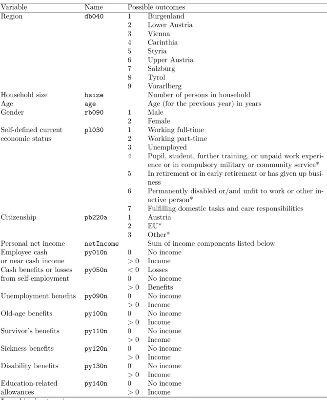
Table2lists and describes the EU-SILC variables used for generating the synthetic population. Some categories of economic status and citizenship, respectively, have been combined due to their low frequency of occurrence; the combined categories are marked with an asterisk (∗). The variables hsize,age and netIncome are not included in the original EU-SILC dataset.
hsizehas been computed by counting the number of persons in each household,ageis derived from the year of birth, and netIncome is the sum of the income components. A complete description of EU-SILC variables can be found inEurostat (2004).
The sampling weights stored ineusilcS(variable rb050) have been divided by a factor 100 to make the package compile more quickly. We use these reduced sampling weights in this contribution to ensure fast execution of the scripts. Simulating only 1/100 of the population of Austria allows the code in this reproducible manuscript (using knitr; Xie 2013) to run in less than one minute. If we were to simulate a population of the size of Austria (> 8 million individuals), it would require us to first multiply the sampling weights by 100. The processing time would be significantly higher, in particular due to the SA procedure described in Sections2.2 and4.9.
In the following example, theeusilcSdataset is saved under the nameorigDatato indicate that it provides the original data used as the starting point when constructing the synthetic population. The dataset contains data on 11,725 individuals and 4,641 households (variable
db030is the household unique identifier): R> set.seed(1234)
Variable Name Possible outcomes Region db040 1 Burgenland 2 Lower Austria 3 Vienna 4 Carinthia 5 Styria 6 Upper Austria 7 Salzburg 8 Tyrol 9 Vorarlberg
Household size hsize Number of persons in household Age age Age (for the previous year) in years
Gender rb090 1 Male
2 Female
Self-defined current pl030 1 Working full-time economic status 2 Working part-time
3 Unemployed
4 Pupil, student, further training, or unpaid work experi-ence or in compulsory military or community service* 5 In retirement or in early retirement or has given up
busi-ness
6 Permanently disabled or/and unfit to work or other in-active person*
7 Fulfilling domestic tasks and care responsibilities Citizenship pb220a 1 Austria
2 EU* 3 Other*
Personal net income netIncome Sum of income components listed below Employee cash py010n 0 No income
or near cash income >0 Income Cash benefits or losses py050n <0 Losses from self-employment 0 No income
>0 Benefits Unemployment benefits py090n 0 No income
>0 Income Old-age benefits py100n 0 No income
>0 Income Survivor’s benefits py110n 0 No income
>0 Income Sickness benefits py120n 0 No income
>0 Income Disability benefits py130n 0 No income
>0 Income Education-related py140n 0 No income allowances >0 Income * combined categories
Dataset name Description Comments
origData Original survey data Included in the package as eusilcS; weights are modified by factor 100 to simulate realistic large populations
census Census data used to produce margins; usually such margins are available from registers
Produced as one realization of a pop-ulation with different seed as the syn-thetic population; needed to produce tables for calibration on gender × re-gion ×economic status
totalsRG Known population totals on re-gion×gender
Obtained from Statistics Austria’s website; used for calibration purposes
districts,
tab
Finer geographical location tab as table holding district × region information; simulated and added to census; used for spatial calibration of the population
synthP Simulated synthetic population simulated from given datasets
synthPadj Calibrated synthetic population simulated from given datasets
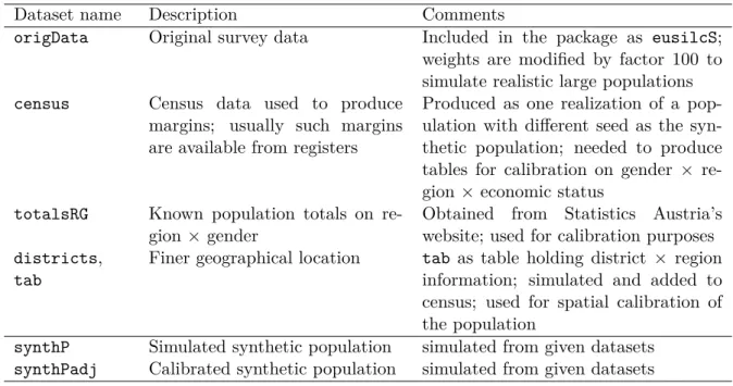
Table 3: Datasets used and simulated in this work. The survey sampleorigDatais central to produce the synthetic populationsynthP; all other datasets are used for calibration purposes.
R> data("eusilcS", package = "simPop") R> origData <- eusilcS
R> dim(origData)
[1] 11725 18
The number of households is:
R> length(unique(origData$db030))
[1] 4641
We also make use of the population numbers by region and gender from the Austrian cen-sus, available from the website of Statistics Austria (http://www.statistik.at/), and also included insimPop. Table3provides a list of all input and output datasets used in the paper. 4.2. Approach used to generate the Austrian synthetic data
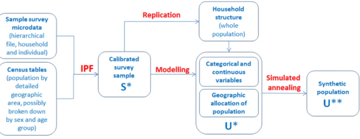
We generate the Austrian synthetic population data using multiple techniques, following the schema presented in Figure 1. This workflow is an adaptation, proposed by Alfons et al.
(2011), of the framework of Münnich and Schürle (2003). As a first step, sampling weights in the survey data are calibrated using the IPF technique to match population numbers in the census tables. The household structure of the synthetic population is then created by extrapolating the calibrated sample. Categorical and continuous variables are added to that structure using a modeling approach. Then the synthetic population is distributed among
Figure 1: Workflow for simulating the population.
small(er) geographic areas. As a last step, the population dataset is re-calibrated, this time using the SA technique.
The proposed framework proceeds in a stepwise fashion, generating categorical variables first, then continuous variables. This sequence is not imposed by simPop and can be modified. Categorical and continuous variables can be simulated in any order, allowing for simulated continuous variables to be used as predictors for simulating categorical variables.
Before simulating variables, we create an object of class ‘dataObj’ that will hold all infor-mation needed to construct the synthetic population. Objects of this class are generated with specifyInput(). We identify the survey microdata to be used as input, and the vari-ables providing information on clustering (here: households), household size, subpopulations (allowing in this case to account for heterogeneities across regions – db040), and sampling weights (variable rb050).
R> inp <- specifyInput(origData, hhid = "db030", hhsize = "hsize", + strata = "db040", weight = "rb050")
A summary of the content of this ‘dataObj’ object is displayed using the print method. R> print(inp)
---survey sample of size 11725 x 19
Selected important variables:
household ID: db030 personal ID: pid
variable household size: hsize sampling weight: rb050
strata: db040
---4.3. Calibration of the sample
Assuming that the sample microdata used as input have not been previously calibrated to the population totals provided by census tables, we calibrate the sample weights by iterative proportional fitting using function calibSample(). Because we are using weights reduced by a factor of 100, as mentioned in Section4.1, we also divide the population totals by 100. Population totals can be provided either as a data frame or as an n-dimensional table (in our example, a two-dimensional table); both will produce identical results, as shown in the following example.
R> data("totalsRG", package = "simPop") R> print(totalsRG) rb090 db040 Freq 1 male Burgenland 140436 2 female Burgenland 146980 3 male Carinthia 270084 4 female Carinthia 285797 5 male Lower Austria 797398 6 female Lower Austria 828087
7 male Salzburg 702539 8 female Salzburg 722883 9 male Styria 259595 10 female Styria 274675 11 male Tyrol 595842 12 female Tyrol 619404
13 male Upper Austria 353910 14 female Upper Austria 368128
15 male Vienna 850596
16 female Vienna 916150
17 male Vorarlberg 184939 18 female Vorarlberg 190343
or as an-dimensional table (in this example, a 2-dimensional table). R> data("totalsRGtab", package = "simPop")
R> print(totalsRGtab)
1 db040
2 rb090 Burgenland Carinthia Lower Austria Salzburg Styria Tyrol
3 female 146980 285797 828087 722883 274675 619404
4 male 140436 270084 797398 702539 259595 595842
5 db040
6 rb090 Upper Austria Vienna Vorarlberg
7 368128 916150 190343
R> totalsRG$Freq <- totalsRG$Freq / 100 R> totalsRGtab <- totalsRGtab / 100
R> weights.df <- calibSample(inp, totalsRG) R> weights.tab <- calibSample(inp, totalsRGtab) R> identical(weights.df, weights.tab)
[1] TRUE
The resulting calibrated weights are added to the ‘simPopObj’ object inp using function
addWeights().
R> addWeights(inp) <- calibSample(inp, totalsRGtab)
4.4. Creating the household structure of the synthetic population
Using the calibrated sample dataset as an input, the household structure of the synthetic population is built by resampling households from the survey microdata. The household structure contains a set of user-defined “basic variables”, typically the age, sex (rb090), and geographic location (rb090) of household members. The data that are added to the synthetic population at this stage are thus data obtained from actual survey respondents. This approach prevents the creation of unrealistic household structures. It is recommended for confidentiality reasons to include as few variables as possible in this phase.
Alias sampling (Walker 1977) is well suited for our purpose, as it is very fast for a large number of sampled elements.
LetxS
hij and xUhij denote the value of person i from householdh in variable j for the sample
and population data, respectively, and let the firstp1 variables contain the basic information on the household structure. For each population household h ∈ HklU, a survey household h0 ∈HS
kl is selected with probabilitywh0/Ph∈HS klwh
and the household structure is set to xUhij :=xSh0ij, i= 1, . . . , l, j = 1, . . . , p1 . (2)
The inp object previously generated is used as input for simStructure(). The function generates the structure of the synthetic population using a replication approach that au-tomatically takes sampling weights into account. The resulting object (synthP) is of class ‘simPopObj’.
R> synthP <- simStructure(data = inp, method = "direct", + basicHHvars = c("age", "rb090", "db040"))
4.5. Adding categorical variables
Using the household structure information and the calibrated weights, categorical variables are added to the synthetic population. Our preferred approach is to construct categorical variables by model-based simulation. Models are fit to the sample data and used to “predict” the new variables (see alsoAlfonset al. 2011;Meindl, Templ, and Kowarik 2014). Synthetic reconstruction provides the following alternative solution.
Model-based simulation of categorical variables
Münnich et al. (2003) and Münnich and Schürle (2003) propose an approach to simulate categorical variables by estimating conditional distributions directly from a rather large sam-ple. Their method does not allow combinations that do not occur in the sample dataset to occur in the synthetic population dataset (Kraft 2009). As a large number of combinations of categories found in the actual population will usually not be found in the sample data, the resulting synthetic population is unlikely to reproduce the variation of combinations. To overcome these shortcomings, Alfons et al. (2011) propose a method that estimates condi-tional distributions using multinomial logistic regression models. One categorical variable is simulated as follows.
(i) The variable to be simulated (response) is selected from the sample S. The variables (including the household structure variables) used as predictors must be present in both the sampleSand the populationU. Other variables (rest) can be simulated afterwards.
sample S= x1,1 x1,2 · · · x1,j x1,j+1 x1,j+2 · · · x2,1 x2,2 · · · x2,j x2,j+1 x2,j+2 · · · .. . ... . .. ... ... ... ... xn,1 xn,2 · · · xn,j xn,j+1 xn,j+2 · · ·
predictors response rest
(ii) The model matrix is built from the predictors available in the sampleS. A multinomial logistic regression is modeled for the sample data with the variable to be simulated as response. This results in the fit of the regression coefficients β.
(iii) For every individual of the selected variable, predict the outcome category ˆxi,j+1, i= 1, . . . , N by using a multinomial regression model.
For each outcome ˆxi,j+1, i= 1, . . . , N, its conditional probabilities for each Rcategory is estimated by ˆ pi1 := 1 1 +PR r=2exp( ˆβ0r+ ˆβ0rxˆi,1+. . .+ ˆβjrxˆi,j) , ˆ pir := exp( ˆβ0r+ ˆβ0rxˆi,1+. . .+ ˆβjrxˆi,j) 1 +PR r=2exp( ˆβ0r+ ˆβ0rxˆi,1+. . .+ ˆβjrxˆi,j) ,
with r = 2, . . . R and ˆβ0r, . . .βˆj−1,r are the estimated coefficients from a multinomial
is: population U = ˆ x1,1 xˆ1,2 · · · xˆ1,j xˆ∗1,j+1 ˆ x2,1 xˆ2,2 · · · xˆ2,j xˆ∗1,j+1 .. . ... . .. ... ... .. . ... . .. ... ... ˆ xN,1 xˆN,2 · · · xˆN,j xˆ∗1,j+1 ˆ β×pred. ≈ xˆ∗j+1
Using multinomial logistic regression models to estimate conditional distributions allows for combinations that do not occur in the sample but are likely to occur in the true population to be created. Such combinations are calledrandom zeros as opposed tostructural zeros, where their occurrences are not possible (e.g., Simonoff 2003).
Categorical variables are simulated using the household structure of the synthetic popula-tion and the sample microdata as input. Both are included in the synthP object of class ‘simPopObj’ previously generated. In our example, we generate categorical variables on eco-nomic status (variable pl030) and citizenship (variable pb220a) by applying the function
simCategorical(). The variables to be simulated are specified in argumentadditional. R> synthP <- simCategorical(synthP, additional = c("pl030", "pb220a"), + method = "multinom", nr_cpus = 1)
Accepted values for argument method are "multinom" (i.e., estimation of the conditional probabilities using multinomial log-linear models and random draws from the resulting dis-tributions); "distribution"(i.e., random draws from the observed conditional distributions of their multivariate realizations); "ctree" and "cforest" (classification trees and classifi-cation using random forest, both from the R package party, Hothorn, Hornik, and Zeileis 2006; Strobl, Boulesteix, Kneib, Augustin, and Zeileis 2008); and "ranger" (random for-est from the R package ranger, Wright and Ziegler 2017). Many additional options can be specified and are described in the help file, ?simCategorical. The function argument
regModel may be discussed in more detail. It allows to specify variables or a model (for each variable to be simulated) that is used when simulating additional categorical variables. If regModel = "basic" (default), only the basic household variables are chosen as predic-tors. IfregModel = "available"all available variables are used as predictors. For example,
regModel = list("basic", "available") of simCategorical would use the basic vari-ables (from simStructure) for simulating (in the previous code listing) the variable pl030
and all available variables (structural/basic ones plus already simulated variables) are used to simulate pb220a. Note that for each variable to simulate, also a formula can be specified. If a formula or a list of formulas are provided, checks are performed if all required variables are available.
Parallel computing is automatically applied. The number of used cores is equal to 1) the number of strata (if specified in specifyInput()), if the number of strata is lower than the number of available CPUs, or 2) the number of cores minus one if the number of strata is equal to or higher than the number of available CPUs. Alternatively, the number of cores for parallel
computing can be specified directly using function argumentnr_cpus(see?simCategorical). Note that running the code repeatedly on the same number of cores gives the same results, however changing the number of cores will change the random results.
The print method displays basic information about the current synthetic population. R> print(synthP)
---synthetic population of size 85057 x 9
build from a sample of size 11725 x 19
---variables in the population:
db030,hsize,age,rb090,db040,pid,weight,pl030,pb220a
In the previous example, we assumed that categorical variables can be predicted independently for each household member. This assumption is not always realistic. The characteristics of an individual will often depend on the characteristics of other members of the same house-hold. For example, the religion of children and other household members will typically be similar to the religion of the head of the household. To take the relationships between house-hold members into account when simulating categorical variables, simPopprovides function
simRelation().
Synthetic reconstruction
We show here how a categorical variable representing the economic status (pl030) is created using the synthetic reconstruction approach. We useeusilcS as the known probability table (in a real application, this information would likely come from a census). We first show how the method is applied to predict values for a specific household.
R> censusInfo <- eusilcS[, c("age", "rb090", "pl030")]
pl030is a variable with seven possible categories. R> stat <- as.numeric(levels(censusInfo$pl030)) R> stat
[1] 1 2 3 4 5 6 7
We generate the conditional probabilities of these categories conditional onageand gender
(variablerb090):
R> tab1 <- prop.table(table(censusInfo))
R> probs <- reshape2::dcast(as.data.frame(tab1),
For each combination values ofageandrb090,probscontains the conditional probability for each of the 7 categories ofpl030. We show the information related to the first household: R> pop <- subset(eusilcS, eusilcS$db030 == 1, select = c("age", "rb090")) R> pop
age rb090 9292 72 male 9293 66 female
We want to sampleeconomic status givenageandrb090and known probabilities. As shown in the following code, we need to merge objects popand probs on variables ageand rb090. Then it is possible to draw – for each individual – a value for economic status given the conditional probabilities which are then available in the merged dataset.
R> pop <- merge(pop, probs, all.x = TRUE)
R> pop$status <- sapply(1:nrow(pop), function(x) { + pp <- pop[x, -c(1:2)]
+ ifelse(all(pp == 0), NA, sample(stat, 1, prob = pp)) + })
R> pop <- pop[, c("age", "rb090", "status")] R> pop
age rb090 status
1 66 female 7
2 72 male 5
This concept is implemented in function simCategorical() using"distribution" as value for argument method. In the following, the code for a real application using synthetic recon-struction is presented in which a new object synthRecof class ‘simPopObj’ is created. R> data("eusilcS", package = "simPop")
R> inp <- specifyInput(data = eusilcS, hhid = "db030", hhsize = "hsize", + strata = "db040", weight = "db090")
R> synthRec <- simStructure(data = inp, method = "direct", + basicHHvars = c("age", "rb090"))
R> synthRec <- simCategorical(synthRec, additional = "pl030", + method = "distribution", nr_cpus = 1)
[1] "age" "rb090"
The first step creates the required input; the second step computes a synthetic population consisting only of basic variables; and the third step generates the additional categorical variablepl030.
4.6. Adding continuous variables
In our example, we will add information onpersonal net income (variable netIncome) to the synthetic datasetsynthP.
Two approaches to simulate continuous variables are implemented insimPop. The first in-volves fitting a multinomial model and random drawing from the resulting categories. This approach is based on the simulation of categorical variables described in the previous section, whereas first the continuous variable is categorized and the multinomial model is estimated, as in the previous section. In the last step, random draws are taken from the intervals of the categories into which predictions at population level fall. In that case, values from the largest categories could be drawn from a generalized Pareto distribution, since the values are not expected to be uniformly distributed.
The second approach is based on a two-step regression model with random error terms. In the first step of this approach, a logistic regression is applied. In the second step, a linear regression is applied only to observations for which the prediction of the logistic regression is closer to one than to zero. This is necessary when considering semi-continuous distributions, otherwise only the linear regression imputation is applied. A random error value is added to avoid all individuals with the same set of predictors receiving the same value for the predicted variables, which would underestimate the variance. Random draws can be based on the normal assumption or, preferably, taken from the regression residuals.
Continuous variables are generated using simContinuous(). Prior to applying the func-tion, the basic household structure and possibly other categorical predictors must have been simulated using simStructure() and simCategorical(), respectively. An object of class ‘simPopObj’ is provided as input. The continuous variables to be generated are specified in function argumentadditional. The function takes additional arguments, which are described in the help file; see?simContinuous.
The following example implements the multinomial model with a random draws approach (the default option for thesimContinuous()function). Variables age category,gender,household size,economic status and citizenshipare used as predictors of personal net income. A model is computed separately for each region. For the categorization of personal net income, zero is a category of its own since personal net income is a semi-continuous variable. Breakpoints for the positive values are chosen as their weighted 1%, 5%, 10%, 20%, 40%, 60%, 80%, 90%, 95% and 99% quantiles. Also, the only three negative values are used as breakpoints for negative income. Values in these categories – the two largest breakpoints – are drawn from a truncated generalized Pareto distribution.
R> synthP <- simContinuous(synthP, additional = "netIncome", upper = 200000, + equidist = FALSE, imputeMissings = FALSE, nr_cpus = 1)
In the EU-SILC data, net income values are conditioned on the age of respondents, and individuals aged less than 16 years do not have an income. We therefore set this variable as missing for the population below an age of 16 years by extracting the information from the ‘simPopObj’ object, imputing the values as missing, and overwriting the object. The population below an age of 16 years is thus not considered in regression models estimating net income of the population aged 16 years and above.
R> ageinc <- pop(synthP, var = c("age", "netIncome")) R> ageinc$age <- as.numeric(as.character(ageinc$age))
R> ageinc[age < 16, netIncome := NA]
R> pop(synthP, var = "netIncome") <- ageinc$netIncome
Alternatively to the multinomial model, the two-step regression model approach could be used, in which case the code would be as follows:
R> synthP <- simContinuous(synthP, additional = "netIncome", method = "lm", + nr_cpus = 1)
In this case, random draws from the residuals are used. Positive values in the sample data are trimmed with parameters α1 =α2 = 0.01 and log-transformed in the second step of the procedure. Trimming is used since this performed better (results not shown, cf.Kraft 2009). To simulate negative income values, a multinomial model can be used in the first step. For negative income values, again, the only three existing values are used as breakpoints and the simulated values are drawn from uniform distributions in the corresponding classes.
4.7. Simulation of components
In household surveys, information on net individual income is typically not collected, but derived from other variables (e.g., from information collected on income by source). A syn-thetically generated continuous variable can be broken down by its components using function
simComponents().
As input, the function requires the sample microdata (which must contain variables represent-ing the components of the variables to be split) and the synthetic data containrepresent-ing household structure, categorical variables, and the continuous variable to be split. This information is contained in the object of class ‘simPopObj’ previously generated usingsimStructure(),
simCategorical()and simContinuous().
The simulation of components of continuous variables of population data is performed by resampling fractions using the survey data at hand. The following code shows how to create income components of variable netIncome. First, we categorize netIncome for use as a conditioning variable.
R> sIncome <- manageSimPopObj(synthP, var = "netIncome", sample = TRUE) R> sWeight <- manageSimPopObj(synthP, var = "rb050", sample = TRUE) R> pIncome <- manageSimPopObj(synthP, var = "netIncome")
R> breaks <- getBreaks(x = sIncome, w = sWeight, upper = Inf, + equidist = FALSE)
R> synthP <- manageSimPopObj(synthP, var = "netIncomeCat",
+ sample = TRUE, set = TRUE, values = getCat(x = sIncome, breaks)) R> synthP <- manageSimPopObj(synthP, var = "netIncomeCat",
+ sample = FALSE, set = TRUE, values = getCat(x = pIncome, breaks)) We now simulate net income components.
R> synthP <- simComponents(simPopObj = synthP, total = "netIncome", + components = c("py010n", "py050n", "py090n", "py100n", "py110n",
+ "py120n", "py130n", "py140n"), conditional = c("netIncomeCat", "pl030"), + replaceEmpty = "sequential", seed = 1)
We print the information of the synthetic population, which shows that the income component variables have been added.
---synthetic population of size 85057 x 19
build from a sample of size 11725 x 20
---variables in the population:
db030,hsize,age,rb090,db040,pid,weight,pl030,pb220a,netIncomeCat,netIncome, py010n,py050n,py090n,py100n,py110n,py120n,py130n,py140n
4.8. Allocating the population in small areas
At this stage, the only information available on the geographic location of the synthetic households is that provided by the strata variable used in the first step of the procedure (the regions, in the case of Austria). This population may be distributed across smaller geographic areas (districts, in the case of Austria) if the distribution of the population at this lower level is available. We simulate smaller regions using functionsimInitSpatial(). In the current implementation of simPop, the function requires at least one of two tables as input, the tables must have exactly three columns. The first two columns contain the identification of the broader (first column) and smaller (second column) geographic areas. The third column contains the known population of the smaller area (as number of persons if provided for parametertspatialPor as number of households for parametertspatialHH). A future improvement will allow users to specifyn-way tables holding distributional information of large and small areas together with other variables, e.g., the population by region, district, and age group (note that in the absence of such an option, calibration after allocating districts can be performed using functioncalibPop()to achieve a similar objective).
Since the EU-SILC data used in this work do not contain information on districts, we gener-ate districts randomly to demonstrgener-ate the functionality ofsimInitSpatial(). We randomly distribute the EU-SILC population to districts assigned to regions. For each region, a num-ber between 10 and 90 is randomly drawn that determines the numnum-ber of districts in the corresponding region.
R> simulate_districts <- function(inp) { + hhid <- "db030"
+ region <- "db040"
+ a <- inp[!duplicated(inp[, hhid]), c(hhid, region)] + spl <- split(a, a[, region])
+ regions <- unique(inp[, region])
+ tmpres <- lapply(1:length(spl), function(x) { + codes <- paste(x, 1:sample(10:90, 1), sep = "")
+ spl[[x]]$district <- sample(codes, nrow(spl[[x]]), replace = TRUE)
+ })
+ tmpres <- do.call("rbind", tmpres) + tmpres <- tmpres[, -2]
+ out <- merge(inp, tmpres, by.x = hhid, by.y = hhid, all.x = TRUE) + invisible(out)
+ }
R> data("eusilcS", package = "simPop") R> census <- simulate_districts(eusilcS) R> head(table(census$district))
11 110 111 112 113 114
20 6 9 19 45 28
Based on this, we generate two tables, one containing the counts of persons by region and the other with the household population by region. (db040) and district.
R> tabHH <- as.data.frame(xtabs(rb050 ~ db040 + district, + data = census[!duplicated(census$db030), ]))
R> tabP <- as.data.frame(xtabs(rb050 ~ db040 + district, data = census)) R> colnames(tabP) <- colnames(tabHH) <- c("db040", "district", "Freq")
These tables are used as an input to add a variable district to the synthetic population dataset. The function simInitSpatial() requires an object of class ‘simPopObj’ as input. The procedure, applied independently to each region, adds a variabledistrict to the syn-thetic population (see last column in the following table).
R> synthP <- simInitSpatial(synthP, additional = "district", + region = "db040", tspatialHH = tabHH, tspatialP = tabP) R> head(popData(synthP), 2)
db030 hsize age rb090 db040 pid weight pl030 pb220a
1: 1 1 53 female Burgenland 1.1 1 7 AT
2: 2 1 37 male Burgenland 2.1 1 1 AT
netIncomeCat netIncome py010n py050n py090n py100n py110n
1: (0,657] 174.1431 0.00 174.1431 0 0 0.000
2: (1.79e+04,2.35e+04] 19598.5668 15441.29 0.0000 0 0 4157.273 py120n py130n py140n district
1: 0 0 0 19
2: 0 0 0 119
4.9. Post-calibration of the synthetic population
Although the sample used as input for the simulation of the synthetic population had been calibrated to known marginals (see Section 4.3), the resulting synthetic population will not exactly match these marginals due to randomness in the data-generation process. If a (quasi-)perfect match to known marginals is a requirement, an SA procedure can be applied using
function calibPop(). The algorithm consists of an iterative search for a (near) optimal combination of households to populate the geographic areas. At each iteration, households are swapped. The sum of absolute differences between target marginals and a synthetic marginal is estimated and used as the objective function to assess whether the swap has or has not resulted in an improvement.
In the following code, we calibrate the synthetic dataset to the known distribution of the population by region,sex, andeconomic status. We obtain this distribution from a synthetic census created for the purpose of our demonstration. In practice, margins will be obtained from actual sources such as population censuses or administrative data. We simulate a census population dataset, from where we derive the “known margins”:
R> census <- simStructure(data = inp, method = "direct", + basicHHvars = c("age", "rb090", "db040"))
R> census <- simCategorical(census, additional = c("pl030", "pb220a"), + method = "multinom", nr_cpus = 1)
We add these margins to our object synthP: R> census <- data.frame(popData(census))
R> margins <- as.data.frame(xtabs(~ db040 + rb090 + pl030, data = census)) R> margins$Freq <- as.numeric(margins$Freq)
R> synthP <- addKnownMargins(synthP, margins)
We then calibrate to these margins using SA with calibPop().
R> synthPadj <- calibPop(synthP, split = "db040", temp = 1, + eps.factor = 0.00005, maxiter = 200, temp.cooldown = 0.975,
+ factor.cooldown = 0.85, min.temp = 0.001, verbose = TRUE, nr_cpus = 1) The SA approach is a very intensive process that is typically applied to small datasets of a few hundred or a few thousand observations, at most. A highly optimized implementation insimPopmakes the algorithm applicable to larger datasets. Parallel computing is applied, exploiting a number of CPUs determined automatically, unless manually specified by the user (see details in?calibPop). But the computation time remains long and depends highly on the chosen parameters. To assess the improvement resulting from the SA procedure, we compare the population numbers byregion,sex, and economic status before and after its application. First, we extract population and synthetic population data:
R> pop <- data.frame(popData(synthP))
R> popadj <- data.frame(popData(synthPadj))
We generate the population tables to be compared and compute the differences. We observe that the non-calibrated population numbers differ (comparingtab.censuswithtab.beforeSA), while applying the SA algorithm results in a perfect match between the two tables (comparing
tab.censuswithtab.afterSA).
R> tab.census <- ftable(census[, c("rb090", "db040", "pl030")]) R> tab_afterSA <- ftable(popadj[, c("rb090", "db040", "pl030")]) R> tab.census - tab_afterSA
pl030 1 2 3 4 5 6 7 rb090 db040 male Burgenland 0 0 0 0 0 0 0 Carinthia 0 0 0 0 0 0 0 Lower Austria 0 0 0 0 0 0 0 Salzburg -1 0 -1 0 -100 -8 -5 Styria 517 26 70 0 627 12 4 Tyrol -1 -3 0 0 0 0 -1 Upper Austria 424 33 11 0 762 1 0 Vienna 0 0 0 0 0 0 0 Vorarlberg 0 0 0 0 0 0 0 female Burgenland 0 0 0 0 0 0 0 Carinthia 0 0 0 0 0 0 0 Lower Austria 0 0 0 0 0 0 0 Salzburg -241 -73 -20 0 -1818 -9 -171 Styria 248 163 2 1 892 0 380 Tyrol 0 -1 0 0 -553 0 0 Upper Austria 88 229 4 0 991 4 356 Vienna 0 0 0 0 0 0 0 Vorarlberg 0 0 0 0 0 0 0
5. Data utility of the simulated population
In a last and critical step, we assess the utility of the generated synthetic population. Data utility can be assessed with two approaches (Reiter 2012): by quantifying some statistical dis-tance between the distributions of the original data and the synthetic files; and by comparing differences in specific models between the original and the synthetic data.
5.1. Data utility according to univariate and multivariate distributions We first check how well univariate distributions are preserved. Given the example from Section4, we see that univariate distributions are preserved very well with the model-based approach. In the following table, we consider variable pl030, the economic status. We calculate the Horwitz-Thompson estimate of counts using the original, unmodified sample data.
R> dat <- data.frame(sampleData(synthP)) R> tableWt(dat$pl030, weights = dat$rb050)
x
1 2 3 4 5 6 7
31320 6250 3010 4238 18425 853 6527
This can be compared with the counts of the synthetic population where the differences are very small:
Data = Sample db040 rb090 hsiz e female 98 7 6 5 4 3 2 1 male B C LA Sl St T UA Vn Vr 98 76 5 4 3 2 1 Data = Population db040 rb090 hsiz e female 98 7 6 5 4 3 2 1 male B C LA Sl St T UA Vn Vr 98 76 5 4 3 2 1
Figure 2: Mosaic plots of gender, region and household size.
R> table(popData(synthP)$pl030)
1 2 3 4 5 6 7
33381 6395 3113 16299 18356 925 6588
The multivariate structure of the simulated categorical variables is evaluated by means of graphical comparison.
R> tab <- spTable(synthP, select = c("rb090", "db040", "hsize"))
R> spMosaic(tab, labeling = labeling_border(abbreviate = c(db040 = TRUE))) Figure 2 contains mosaic plots visualizing the expected and realized frequencies of gender (rb090), household sizes (hhsize), and region (db040).
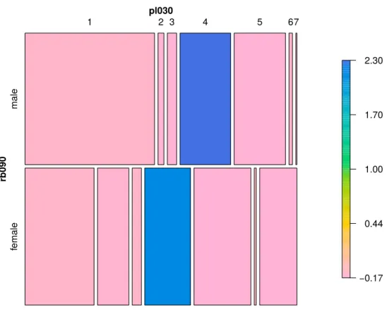
Figure 3 shows a mosaic plot of gender (rb090) and economic status (pl030) with slightly different graphical options.
R> tab <- spTable(synthP, select = c("rb090", "pl030")) R> spMosaic(tab, method = "color")
−0.17 0.44 1.00 1.70 2.30 pl030 rb090 female male 1 2 3 4 5 67
Figure 3: Colored mosaic plot of gender and economic status.
Function spTable() performs the cross-tabulation on the sample (Horwitz-Thompson esti-mates) and population levels for selected variables. spMosaic() plots the frequencies; on the left-hand side is the sample data, and on the right-hand side, values of the synthetic population. We note that both plots show very similar structures for sample and population data. While the two plots at the top of Figure2 are nearly identical, closer inspection of the two plots at the bottom reveals small differences, which result from the multinomial logistic regression models.
In general, the following two points need to be kept in mind. First, expected frequencies of different combinations are solely determined by the sum of the corresponding sample weights. Second, multinomial models allow simulating combinations that do not occur in the sample but are likely to occur in the population. Consequently, differences may be interpreted as corrections of the expected frequencies.
Figure 3 shows the relative differences of expected (i.e., estimated) and realized (i.e., sim-ulated) population sizes for gender (rb090) × economic status (pl030). Only very small differences occur for small categories, e.g., for males with economic status 6 or 7. The real-ized population is slightly smaller (<1.2%) than the estimated sample population size. For additional results on the simulation of categorical variables in the case of EU-SILC, including two goodness-of-fit tests, seeKraft(2009).
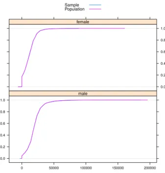
For simulating personal net income, two approaches were described in Section4.6. In Figure4, we compare the cumulative distribution function (CDF) of personal net income (netIncome) by gender (rb090) obtained from the synthetic population, with the empirical CDF from the
0.0 0.2 0.4 0.6 0.8 1.0 0 50000 100000 150000 200000 male 0.0 0.2 0.4 0.6 0.8 1.0 female Sample Population
Figure 4: Cumulative distribution functions of personal net income. For better visibility, only the main parts of the data are shown.
original sample population.
R> spCdfplot(synthP, "netIncome", cond = "rb090", layout = c(1, 2))
Sample weights are taken into account by adjusting the step height. For better visibility of differences in the distribution, the plot shows only the main part of the data, from 0 to the weighted 99% quantile of the positive values in the sample. The CDFs indicate an excellent fit.
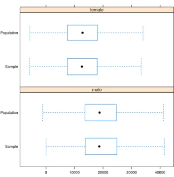
Figure5 uses box plots to compare the distributions of personal net income (netIncome) by gender (rb090).
R> spBwplot(synthP, x = "netIncome", cond = "rb090", layout = c(1, 2))
Box and whiskers are adapted for semi-continuous variables; they are computed only for the non-zero part of the data and the box widths are proportional to the ratio of non-zero observations to the total number of observed values. For the sample data, sample weights are taken into account when computing the box plot statistics and box widths. Figure6compares the CDF ofnetIncome for the sample and population based on region (db040). Again, we observe an almost perfect fit.
R> spCdfplot(synthP, "netIncome", cond = "db040", layout = c(3, 3))
These box plots suggest that the proposed approaches perform well. The proportions of zeros and the distribution of non-zero observations seem to be well reflected in the simulated pop-ulation. This underlines the good fit of the models and illustrates that the proposed methods succeed in accounting for heterogeneities in the data. Additional results from simulations of
Sample Population 0 10000 20000 30000 40000 ● ● male Sample Population ● ● female
Figure 5: Box plots of personal net income. Extreme values are omitted.
0.0 0.2 0.4 0.6 0.8 1.0 0 50000 150000 Burgenland Carinthia 0 50000 150000 Lower Austria Salzburg Styria 0.0 0.2 0.4 0.6 0.8 1.0 Tyrol 0.0 0.2 0.4 0.6 0.8 1.0 Upper Austria 0 50000 150000 Vienna Vorarlberg Sample Population