Article
Dissolved Inorganic Geogenic Phosphorus Load to
a Groundwater-Fed Lake: Implications of Terrestrial
Phosphorus Cycling by Groundwater
Catharina Simone Nisbeth1, Jacob Kidmose2, Kaarina Weckström2,3, Kasper Reitzel4 , Bent Vad Odgaard5, Ole Bennike2, Lærke Thorling2 , Suzanne McGowan6,
Anders Schomacker7,8 , David Lajer Juul Kristensen1and Søren Jessen1,*
1 Department of Geosciences and Natural Resource Management (IGN), University of Copenhagen, Øster Voldgade 10, 1350 Copenhagen K, Denmark; csnm@ign.ku.dk (C.S.N.); dlajer@gmail.com (D.L.J.K.) 2 Geological Survey of Denmark and Greenland (GEUS), Øster Voldgade 10, 1350 Copenhagen K, Denmark;
jbki@geus.dk (J.K.); kaarina.weckstrom@helsinki.fi (K.W.); obe@geus.dk (O.B.); lts@geus.dk (L.T.) 3 Ecosystems and Environment Research Programme (ECRU)/Helsinki Institute of Sustainability Science,
P.O. Box 65 (Viikinkaari 1), 00014, University of Helsinki, Yliopistonkatu 4, 00100 Helsinki, Finland 4 Institute of Biology, University of Southern Denmark, Campusvej 55, DK-5230 Odense M, Denmark;
reitzel@biology.sdu.dk
5 Institute of Geoscience, University of Aarhus, Høegh-Guldbergs Gade 2, 8000 Aarhus C, Denmark; bvo@geo.au.dk
6 School of Geography, University of Nottingham, University Park Nottingham NG7 2RD, UK; suzanne.mcgowan@nottingham.ac.uk
7 Natural History Museum of Denmark (SNM), Øster Voldgade 5-7, 1350 Copenhagen K, Denmark; anders.schomacker@bio.ku.dk
8 Department of Geosciences, UiT The Arctic University of Norway, Postboks 6050 Langnes, N-9037 Tromsø, Norway
* Correspondence: sj@ign.ku.dk
Received: 28 June 2019; Accepted: 16 October 2019; Published: 24 October 2019
Abstract: The general perception has long been that lake eutrophication is driven by anthropogenic sources of phosphorus (P) and that P is immobile in the subsurface and in aquifers. Combined investigation of the current water and P budgets of a 70 ha lake (Nørresø, Fyn, Denmark) in a clayey till-dominated landscape and of the lake’s Holocene trophic history demonstrates a potential significance of geogenic (natural) groundwater-borne P. Nørresø receives water from nine streams, a groundwater-fed spring located on a small island, and precipitation. The lake loses water by evaporation and via a single outlet. Monthly measurements of stream, spring, and outlet discharge, and of tracers in the form of temperature,δ18O andδ2H of water, and water chemistry were conducted. The tracers indicated that the lake receives groundwater from an underlying regional confined glaciofluvial sand aquifer via the spring and one of the streams. In addition, the lake receives a direct groundwater input (estimated as the water balance residual) via the lake bed, as supported by the artesian conditions of underlying strata observed in piezometers installed along the lake shore and in wells tapping the regional confined aquifer. The groundwater in the regional confined aquifer was anoxic, ferrous, and contained 4–5µmol/L dissolved inorganic orthophosphate (DIP). Altogether, the data indicated that groundwater contributes from 64% of the water-borne external DIP loading to the lake, and up to 90% if the DIP concentration of the spring, as representative for the average DIP of the regional confined aquifer, is assigned to the estimated groundwater input. In support, paleolimnological data retrieved from sediment cores indicated that Nørresø was never P-poor, even before the introduction of agriculture at 6000 years before present. Accordingly, groundwater-borne geogenic phosphorus can have an important influence on the trophic state of recipient surface water ecosystems, and groundwater-borne P can be a potentially important component of the terrestrial P cycle.
Water2019,11, 2213 2 of 23
Keywords: geogenic phosphorus; dissolved inorganic orthophosphate; transport; eutrophication; groundwater-surface water interaction
1. Introduction
Eutrophication poses a major threat to freshwater lake ecosystems worldwide [1–3] and is assumed to be particularly controlled by input of phosphorus (P) [4,5]. Identifying the different pathways of P transport within catchments and determining their relative importance is crucial for optimal freshwater ecosystems management [6–9]. The general perception is that surface and near-surface hydrological pathways are the main transport routes for external P. This is due to the common assumption that P is retained readily in the aquifer sediments by adsorption and metal complex precipitation, predominantly in the oxic zone [10–12].
Over the last few decades, however, evidence of groundwater-transported P has increased [7–9,13–16], indicating that P is not necessarily immobilized in aquifers. Furthermore, there has been increasing awareness that P-rich groundwater can play an important role regarding the trophic state of lakes [14,17–19] especially for groundwater-fed aquatic systems [8,9,17,18]. Even in cases where groundwater only makes up a minor part of the lake’s annual water budget, it can still control the trophic state of the lake, if the discharging groundwater contains a high concentration of P [6,20,21].
The geochemical environment in the aquifer may play an important role regarding the mobilization of P within the aquifer. Walter [13] found that P was mobile in groundwater in two distinct geochemical environments: (1) In anoxic environments with a high concentration of dissolved ferrous iron, and (2) in suboxic environments where a continued phosphorus loading has filled all available sorption sites. Phosphorus may also be mobile in oxic environments with low iron concentrations or if the iron is immobilized as FeS. This is consistent with the recorded correlation between sediment redox conditions and mobilization of inorganic P, where the main mechanisms responsible for sediment P release is reductive dissolution of Fe-oxides [11,12,22].
In many studies [7–9,13–15,17–19] the source of P in the groundwater, discharging to a lake, is either shown or expected to be anthropogenic, or it remains undetermined whether the P source is natural or anthropogenic. However, total phosphorus (TP) concentrations above the 0.3µM (10µg P/L) threshold for oligotrophic freshwater environments [23] have been recorded in deeper, reduced aquifers [8], where P is highly unlikely to be derived from anthropogenic activities. If groundwater from these aquifers discharges into a lake, naturally released (i.e., geogenic) groundwater-borne P may contribute significantly to the trophic state of the lake [24].
The objective of the current study was to investigate whether geogenic groundwater-borne P can be the dominant external contributor of P. This was done by (1) determining the water budget of a Danish lake, Nørresø, (2) investigating the different water-borne external sources of P, and calculating their relative contributions. In order to put the year-long study into a long-term context the results were (3) combined with results of a parallel paleolimnological study.
The internal release of P, which may play an important factor controlling the concentrations of soluble P in the water column [23,25,26], and thus biotic populations during summer blooms, was not included in the present study. Rather, this paper focuses on the identification of the original, external source of the phosphorus now accumulated in the lake and its sediment.
2. Materials and Methods 2.1. Study Site
Brahetrolleborg Nørresø (55◦0805000 N, 10◦2204000 E, hereafter for simplicity termed Nørresø) is a lake located in a clay till moraine landscape. The lake formed during the final stage of the Weichselian glaciation [27], in the southwestern part of Fyn, Denmark (Figure1). Historical maps show
that the topographical catchment of Nørresø was dominated by forest through at least the past two centuries [28].
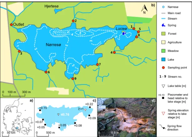
Nørresø is Fyn’s third largest lake, with a geographical surface area of 69.3 ha, including a small island, Lucieø (0.14 ha), located in the eastern end of the lake. The lake has a mean and maximum water depth of 2.3 m and 5.7 m [29], respectively, and the current annual mean elevation of the lake water table is 40.76±0.1 m (seasonal variation) above sea level (ASL).
Visual inflow of water to the lake can be observed from a natural spring elevated 1 m above the lake’s water level, located on the island, Lucieø (Figure1d). The Lucieø spring is simply referred to as “the spring” in this paper. In addition, nine small streams discharge into the lake. They are, for the purpose of this paper, numbered according to their importance in relation to the determined dissolved inorganic orthophosphate (DIP) loading (kg P/yr), with stream 1 and stream 9 representing, respectively, the highest and the lowest external DIP load. Seven of the streams are ephemeral (Nos. 2 and 4–9), whereas the last two streams (Nos. 1 and 3) and the spring feed water to the lake all year round. The perennial stream 1 receives drainage from a meadow, while the ephemeral stream 2 drains a small lake, Hjertesø, north of Nørresø. Hence the P-loading from stream 2 probably reflects the P-cycling processes within Hjertesø. Just one stream (No. 3) receives water from drainage pipes connected to a large agricultural field located west of Nørresø (Figure1b). Water is only discharging from the lake via one surface water outlet located at the western end of the lake.
Water 2019, 11, x FOR PEER REVIEW 3 of 24
Nørresø is Fyn’s third largest lake, with a geographical surface area of 69.3 ha, including a small island, Lucieø (0.14 ha), located in the eastern end of the lake. The lake has a mean and maximum water depth of 2.3 m and 5.7 m [29], respectively, and the current annual mean elevation of the lake water table is 40.76 ± 0.1 m (seasonal variation) above sea level (ASL).
Visual inflow of water to the lake can be observed from a natural spring elevated 1 m above the lake’s water level, located on the island, Lucieø (Figure 1d). The Lucieø spring is simply referred to as “the spring” in this paper. In addition, nine small streams discharge into the lake. They are, for the purpose of this paper, numbered according to their importance in relation to the determined dissolved inorganic orthophosphate (DIP) loading (kg P/yr), with stream 1 and stream 9 representing, respectively, the highest and the lowest external DIP load. Seven of the streams are ephemeral (Nos. 2 and 4–9), whereas the last two streams (Nos. 1 and 3) and the spring feed water to the lake all year round. The perennial stream 1 receives drainage from a meadow, while the ephemeral stream 2 drains a small lake, Hjertesø, north of Nørresø. Hence the P-loading from stream 2 probably reflects the P-cycling processes within Hjertesø. Just one stream (No. 3) receives water from drainage pipes connected to a large agricultural field located west of Nørresø (Figure 1b). Water is only discharging from the lake via one surface water outlet located at the western end of the lake.
Figure 1. (a) Location of the Lake Nørresø in the southern part of Fyn, Denmark. (b) Overview of the numbering of streams, and the locations of stream sampling points and the outlet. The locations of the small island, Lucieø, hosting a spring and the small lake, Hjertesø, are also indicated. The dashed white lines indicate lake bathymetry (in meters;[29]). (c) The relative hydraulic head in seven piezometric wells placed at ~3 m depth. (d) Photo of the spring on the island Lucieø (black arrows indicate flow direction). Iron-oxides stain the bed of the 4-m-long stream which connects the spring to the lake.
Lake stratification has not been observed in Nørresø [27,29], most likely due to the shallow depth relative to the surface area combined with exposure to westerly winds; the lake is therefore assumed to be a well-mixed lake.
2.2. Data Collection
Figure 1.(a) Location of the Lake Nørresø in the southern part of Fyn, Denmark. (b) Overview of the numbering of streams, and the locations of stream sampling points and the outlet. The locations of the small island, Lucieø, hosting a spring and the small lake, Hjertesø, are also indicated. The dashed white lines indicate lake bathymetry (in meters; [29]). (c) The relative hydraulic head in seven piezometric wells placed at ~3 m depth. (d) Photo of the spring on the island Lucieø (black arrows indicate flow direction). Iron-oxides stain the bed of the 4-m-long stream which connects the spring to the lake.
Lake stratification has not been observed in Nørresø [27,29], most likely due to the shallow depth relative to the surface area combined with exposure to westerly winds; the lake is therefore assumed to be a well-mixed lake.
Water2019,11, 2213 4 of 23
2.2. Data Collection
During a year-long study starting in June 2016 and ending in June 2017, a variety of different methods were applied to investigate the lake, according to the objective of this study. In order to understand the hydrogeology and determine the water budget, four different techniques were used: (1) Observations of lithology (including hand drillings and hydrogeophysics), (2) hydraulic head, (3) discharge measurement (from the outlet, spring, and streams), and (4) a water budget equation (using data obtained through the current study and precipitation and evaporation data extracted from a database). Distinction between streams fed with groundwater from a deep regional confined aquifer as opposed to surface runoffwater or groundwater from shallower circulation systems was based on values ofδ18O andδ2H of water combined with the chemical speciation and temperature of the water matrix.
The only bioavailable form of P is orthophosphate (PO43−), which is the dominant P species in DIP [30]. The focus was, therefore, on the external water-borne DIP loadings. This is further justified as the majority of P entering Nørresø is dissolved inorganic P (cf. [31]). It is, therefore, assumed that TP mainly consisted of DIP and thus the measured DIP concentrations were representative of P entering Nørresø (i.e., particulate P and organic P is of secondary importance; further discussion in Section4). Quantification of the external DIP loads from the different external water-borne sources were calculated by multiplication of each source’s monthly discharge and associated measured DIP concentration summed over a year. The methods of investigation are further described below.
2.2.1. Lithology
The surficial geology close to the lake shore and on Lucieø was mapped from 13 hand drillings using an Eijkelkamp hand auger and one Geoprobe®(Salina, Kansas) drilling (see Figure2for locations and lithological logs). Eleven of the drillings penetrated to 2 m depth, two went down to 5 m depth, and the Geoprobe®drilling was 20 m deep. A broader understanding of the geological setting was obtained from lithological logs from three nearby water supply wells (Figure2) for which data were extracted from the Danish borehole JUPITER-database [32]. The three water supply wells all are less than 3 km from the spring and penetrate down to a confined glaciofluvial sand aquifer (screen depths within 42–58 m below terrain).
Water 2019, 11, x FOR PEER REVIEW 4 of 24
During a year-long study starting in June 2016 and ending in June 2017, a variety of different methods were applied to investigate the lake, according to the objective of this study. In order to understand the hydrogeology and determine the water budget, four different techniques were used: (1) Observations of lithology (including hand drillings and hydrogeophysics), (2) hydraulic head, (3) discharge measurement (from the outlet, spring, and streams), and (4) a water budget equation (using data obtained through the current study and precipitation and evaporation data extracted from a database). Distinction between streams fed with groundwater from a deep regional confined aquifer as opposed to surface runoff water or groundwater from shallower circulation systems was based on values of 18O and 2H of water combined with the chemical speciation and temperature of the water
matrix.
The only bioavailable form of P is orthophosphate (PO43−), which is the dominant P species in
DIP [30]. The focus was, therefore, on the external water-borne DIP loadings. This is further justified as the majority of P entering Nørresø is dissolved inorganic P (cf. [31]). It is, therefore, assumed that TP mainly consisted of DIP and thus the measured DIP concentrations were representative of P entering Nørresø (i.e., particulate P and organic P is of secondary importance; further discussion in Section 4). Quantification of the external DIP loads from the different external water-borne sources were calculated by multiplication of each source’s monthly discharge and associated measured DIP concentration summed over a year. The methods of investigation are further described below.
2.2.1. Lithology
The surficial geology close to the lake shore and on Lucieø was mapped from 13 hand drillings
using an Eijkelkamp hand auger and one Geoprobe® (Salina, Kansas) drilling (see Figure 2 for
locations and lithological logs). Eleven of the drillings penetrated to 2 m depth, two went down to 5
m depth, and the Geoprobe® drilling was 20 m deep. A broader understanding of the geological
setting was obtained from lithological logs from three nearby water supply wells (Figure 2) for which data were extracted from the Danish borehole JUPITER-database [32]. The three water supply wells all are less than 3 km from the spring and penetrate down to a confined glaciofluvial sand aquifer (screen depths within 42–58 m below terrain).
Figure 2. Overview of Nørresø and the surrounding area, and locations of piezometers, electrical resistivity tomography (ERT) profiles and the lakebed sediment core site. Lithological logs from the drillings (simplified to combine the shallow peat and the underlying clay till) and water supply wells are also included.
Figure 2. Overview of Nørresø and the surrounding area, and locations of piezometers, electrical resistivity tomography (ERT) profiles and the lakebed sediment core site. Lithological logs from the drillings (simplified to combine the shallow peat and the underlying clay till) and water supply wells are also included.
In addition, two electrical resistivity tomography (ERT) profiles northeast (NE ERT) and southeast (SE ERT) of the lake, i.e., close to Lucieø (Figure2) were conducted (Supplementary Materials Section S1 and Figure S1). Interpretation of the inverted data was based on literature resistivity values [33]. 2.2.2. Hydraulic Heads
Local interaction between surface water and groundwater can be detected by observations of vertical piezometeric head gradients [34]. Thus, seven piezometers were installed at the lakeshore (Figure1c) using a pneumatic hammer. They were all placed in clay till and their 10-cm-long screen was installed typically 3 m but up to 12 m below surface. The hydraulic head was measured using a Solinst 101 water level meter or a Solinst 102 coaxial cable fitted with a P4 probe. Elevation of reference points was recorded using a Trimble differential GPS.
The lake water table was measured every 4 hours using two Onset®pressure transducers with an auto logger function (HOBO Water Level 300
U20L-01). The pressure transducers were installed at the eastern and western lakeshore. A third similar pressure transducer, installed on land, was used to correct for the atmospheric pressure.
The direction of the underground flow in the confined sand aquifer was estimated based on hydraulic head measurements recorded in the JUPITER-database [32].
2.2.3. Water Budget Equation
A general lake water budget equation can be written in the form [35]:
0=N+Sin+GWin−E−Sout−GWout+∆St (1) where N is precipitation, Sin is surface water input (stream discharge in streams 1–9), GWin is groundwater input, E is evaporation, Soutis surface water output, GWoutis groundwater output, and∆St denotes storage change.
Groundwater discharge to the lake (GWin) was divided into two components: Measured groundwater flow (GWmeas) and an estimated groundwater input (GWest) calculated as the residual of the water balance. GWmeasincludes the spring and stream 1. Discussion of this, and other assumptions regarding the water budget components, is presented in Section4. Precipitation (N) and evaporation (E) values for the catchment were extracted from a database compiled by the Danish National Monitoring Program for Aquatic Environment and Nature [36], where the potential evaporation are quantified based on a modified Makkink equation. The used data are from a 20 × 20 km gridded dataset
interpolated from the Danish Metrological Institute’s automated climate stations. The interpolations of potential evaporation for the grid-cell of Nørresø are based on the stations Assens (55◦150N, 9◦530E) 32 km WNW of Nørresø, Årslev (55◦190N, 10◦260E) 18 km NNE of Nørresø, and Sydfyns Flyveplads (55◦010N, 10◦340E) 18 km SE of Nørresø. The climate stations measure hydrological variables every 10 min. The gridded values used for the study were daily averages for the investigated period. Storage change (∆St) in the lake was calculated from the average monthly lake water table variation. 2.2.4. Frequency of Collection of Hydrological and Hydrochemical Data
Stream discharge (Q) measurements and water sampling were conducted concurrently on a monthly basis throughout one hydrological year (6 June 2016–21 June 2017) from all streams with a discharge above quantification limit (1 L/min), as well as from the spring and the outlet. Attempts to increase stream discharge measurement frequency via high-frequency monitoring of stream water level (h) using data logger-equipped pressure transducers were unsuccessful. For a successful Q/h-relation to be established, h needs to be controlled by Q. However, water levels in the streams were less affected by stream discharge than by accumulation of leaves and other organic debris in the streams, and by its high-precipitation-event-based removal by flushing or by humans as part of routine stream management.
Water2019,11, 2213 6 of 23
2.2.5. Outlet, Spring, and Stream Discharge
A cutthroat flume from Baski, Inc. (Englewood, CO, USA) [37,38] equipped with 6.500entrance wing walls was used to measure stream discharge of the outlet (Sout; 800throat width), and the spring and streams 1–9 (Sin; 100throat width).
Triplicate measurements for determination of uncertainty of individual 100 throat width Baski flume measurements were conducted twice in stream 3, once in stream 5 and once in the spring, at conditions representing nearly the full range of stream flow measurements (not including the outlet), from ~6 L/min (stream 3, June 2017) to 64 L/min (stream 9, December 2016). For each uncertainty determination, measurements were carried out within 30 min at three locations a few meters apart each other along each stream.
The uncertainty expressed as one standard deviation (σ) as a function of the discharge rate (Q) determined by the cutthroat flume was found by linear regression which resulted in the equation σ=0.157×Q (r2=0.99). This equation was then used to determineσfor each specific discharge rate
measurement (Figure 6).
2.2.6. Water Sampling and Analysis
All water samples were filtered in the field with 0.22µm Minisart Sartorius cellulose acetate membrane filters directly into polyethylene vials. Samples for DIP and Fe2+analysis were preserved with 0.1 mL 2 M H2SO4per 5 mL water and ferrozine per 3 mL water, respectively.
Determination of Fe2+and DIP were done spectrophotometrically in the laboratory according to the methods of Stookey [39] and Murphy and Riley [40], respectively. Initially, we also measured the S−2concentration. However, none of the samples contained any S−2, hence sampling for S−2 was discontinued.
Major cations (Ca2+, Mg2+, Na+, K+,and NH
4+) and anions (F − , Cl−, Br−, NO3 −, and SO42 − ) were analyzed using ion chromatography (IC) and alkalinity was measured by Gran-titration. These analyses were conducted at the hydrogeochemical laboratory at the Section of Geology, University of Copenhagen, Denmark.
The stable isotopesδ18O andδ2H were analyzed on a Picarro Cavity Ring-Down Spectrometer (CRDS) L2120-i at the Geological Survey of Denmark and Greenland, Copenhagen. Standard deviations were equal to or lower than 0.18%forδ18O and 0.45%forδ2H.
DIP, Fe2+, O2, and temperature data of the water matrix in the water supply wells were extracted from the JUPITER-database [32] and assumed representative of the confined aquifer (i.e., representing deep groundwater). Water samples collected from the east and west end of the lake were combined with outlet samples under the term ‘lake’ in the remainder of the paper as the lake is assumed to be well mixed.
Aqueous speciation and saturation index calculations were done using the free software PHREEQC 3.0 developed by David L. Parkhurst and C.A.J. Appelo (United States Geological Survey, Denver, Colorado, USA).
2.2.7. Field Measurements
Measurements of dissolved O2were conducted in the field using a WTW oxi-3310 IDS Portable Dissolved Oxygen Meter (accuracy:±0.5% of value). Values were recorded upon complete stabilization.
Temperature was read from the probe. Calibration of the probe was performed in the field in the morning before use. pH and electrical conductivity were measured but are not reported in this paper since there were no significant differences internally between the streams and the spring.
2.2.8. Paleolimnological Analyses
The parallel paleolimnological study conducted within the overall project presents results based on diatom, plant pigment, and pollen analyses of a 6-m-long sediment core section sampled in the center of the lake (Figure2). These 6 m of the core consist of gyttja accumulated since about 7500 cal yr BP.
The core chronology is based on accelerator mass spectrometry (AMS) radiocarbon dating of terrestrial plant remains (to avoid hard-water effects) found in the Nørresø sediment core. The obtained radiocarbon ages were calibrated to calendar ages (cal yr BP) using IntCal13 [41]. The first obtained ages are presented in this study, while more sediment samples, to allow for a more detailed chronology, are currently being dated.
Elements were analyzed via X-ray fluorescence (XRF) using an ITRAX core scanner (COX Analytical Systems, Mölndal, Sweden). The scanning of the core was performed at the Natural History Museum of Denmark. To normalize the XRF data in order to compensate for the effects of water content, organic matter, and compaction of the sediment through depth, all data were divided with the total scatter (Rhodium incoherent+Rayleigh). A moving average of five neighboring points was calculated for all elements.
Diatom samples were prepared from ca. 0.2 g of freeze-dried sediment, which was prepared following standard methodologies [42]. Briefly, the sediment was oxidized at 90 ◦C for 6 hours using hydrogen peroxide (H2O2, 30%) in order to remove organic material. Carbonates were then dissolved by addition of a few drops of HCl (35%). The test tubes in which samples were treated were subsequently filled with distilled water and left to settle for 12 h. Residues were then washed several times using demineralized water. A few drops of the final suspension were dried on a cover slip and subsequently mounted in Naphrax®for identification, which was conducted using an optical microscope (Leica DMLB), equipped with phase contrast, at a magnification of×1000.
Pigments were quantitatively extracted in an acetone:methanol:water (80:15:5) mixture. Extracts were left overnight at−10◦C, filtered with a polytetraflourethylen (PTFE) 0.2µm filter and dried under
nitrogen gas. A known quantity was re-dissolved into an injection solution of a 70:25:5 mixture of (1) acetone, (2) ion-pairing reagent (IPR; 0.75 g of tetra butyl ammonium acetate and 7.7 g of ammonium acetate in 100 mL water), and (3) methanol and injected into a high-performance liquid chromatography (HPLC) unit. Pigment extracts were separated using an Agilent 1200 series separation module with quaternary pump. The mobile phase consisted of solvent A (80:20 methanol: 0.5 M ammonium acetate), solvent B (9:1 acetonitrile: water), and solvent C (ethyl acetate) with the stationary phase consisting of a Thermo Scientific ODS Hypersil (Thermo Fisher Scientific, Waltham, MA, USA) column (205×4.6 mm;
5µm particle size). Eluted pigments passed through a photo-diode array detector and UV-visible spectral characteristics were scanned at between 350 and 750 nm. Quantification was based on scanning peak areas at 435 nm and calibrating to a set of commercial standards (DHI LAB Products, Hørsholm, Denmark). Pigment concentrations are reported as molecular weights of pigments in nanomoles per unit dry weight of sediments.
Samples for pollen analysis were prepared from 1 cm3of sediment following Faegri & Iversen [43]. Briefly, 37% HCl was used to remove calcium carbonate and samples rinsed 3 times before boiling in a water bath in centrifugal tubes in 10 mL 10% KOH for about 10 min. After rinsing twice with water, 10 mL concentrated HF (40%) was added and the samples boiled in a water bath for 20–25 min. The samples were then centrifuged and rinsed once with 10 mL 10% HCl and once with water, before 10 mL of concentrated acetic acid was added and the samples were rinsed. This was followed by acetolysis. Finally, the samples were suspended in tert-butanol and transferred to a preparation glass. Drops of silicon oil (AK 2000) were added, before placing the samples for evaporation in a heating cabinet at 50◦C for 2 days. Pollen was counted using a light microscope at a magnification of×400,
higher magnification (×1000) was used for identifying taxonomically difficult pollen types. At least
300 terrestrial pollen grains were counted per sample. The pollen sum, which the percentages are based on, includes all terrestrial pollen taxa.
Water2019,11, 2213 8 of 23
3. Results 3.1. Lithology
In general, the 13 hand drillings all showed two types of sediment: A 0.2–0.7 m thick top layer of peat (not shown in Figure2) followed by grey clay-rich till (seen in Figure2). The lower boundary of the till was not detected. The grey color of the till indicated reduced conditions. The same clay till was also found in the 20 m deep Geoprobe® drilling and in the lithological logs of the three water supply wells. The water supply wells all penetrate a≥35 m thick layer of clay till which confines a
deep anoxic glaciofluvial sand aquifer. Furthermore, clay till was indicated by slow (few months) equilibration of hydraulic pressures in the piezometers screened at up to 12 m below ground. The two ERT profiles (located close to the spring) underlined the occurrence of a thick clay layer (>15 m) confining a sand layer. However, the ERT profiles also indicated that the deep-lying sand layer appears to be connected to the terrain through a thin sloping sand layer (Figure S1 in Supplementary Materials). Hence, the spring could possibly be connected to the deep confined regional aquifer via such sand layers.
3.2. Hydraulic Heads
Groundwater flow in the underlying confined aquifer is toward the southwest. Hydraulic heads in the regional aquifer (42–49 m ASL) were 1–8 m higher than the lake level (40.76 m ASL), resulting in upward hydraulic gradients. The upward gradients were confirmed in all seven of the lakeshore piezometers which had water levels ranging from 0.05–0.22 m above the lake level (Figure1c). 3.3. Water Samples
3.3.1. Stable Isotopes of Water
The isotopic composition of the lake differed significantly from that of the streams, the spring, and the confined aquifer. Lake water samples had the most enriched values ofδ2H (−38.1%to−0.9%)
andδ18O (−5.0%to−3.2%) as well as the largest seasonal variation (Figure3a). However, during no
season did the lake water isotopic signature overlap with that of the other groups. The isotope data plotted along a line with a distinctly lower slope (~5) than that of the local meteoric water line (LMWL, δ2H=7.48×δ18O+5.36; [44]). This can be explained by the lake’s relatively long hydraulic retention time of 1.6 years, which enabled evaporation to significantly enrich the isotopic composition.
The nine streams, the spring, and the confined aquifer were subdivided into three groups according to their isotopic composition; the subdivision is shown in Figure3b,c, which are subsets of Figure3a. Isotopic group 1 represents the samples where the isotope compositions were almost stable throughout the year. Group 1 consists of stream 1, the spring, and the confined aquifer where theδ2H andδ18O (mean δ2H=−58.2%,−58.3%, and−57.9%, respectively, meanδ18O=−8.6%for all three) are
significantly depleted relative to rest of the streams and clusters within a relatively narrow range (1 std. dev. (σ) forδ2H is 0.3–0.4%, and 0.2%forδ18O), thus indicating a shared source of water between these three sources. Isotopic group 2 consists of streams 3, 5, 6, 8, and 9. Their isotopic composition lies likewise within a relatively narrow range (σforδ2H is 0.8–0.9%, and 0.1–0.3%for δ18O), though isotopically enriched (meanδ2H are−52.7%,−53.0%,−52.4%,−52.9%, and−52.6%,
respectively, and meanδ18O is−7.9%for all five sources) relative to group 1 (Figure3b). Isotopic group
3 consists of streams 2, 4, and 7 and represents the three streams with the largest seasonal variation (σforδ2H is 1.5–2.8%, and 0.3–0.6%forδ18O).
Stream 2 stands out in particular with signatures ranging from−57.7%to−47.2%forδ2H and
−8.4%to−6.3%forδ18O, thus containing the isotopically heaviest water of the streams and spring
(Figure3b,c). The stream 2 data, moreover, plot along a line with a lower slope than the LMWL, indicating an evaporation trend similar to that of the lake water in Nørresø (Figure3a). This is consistent with stream 2 seasonally getting water from the small lake, Hjertesø (cf. Figure1b).
Theδ-values of isotopic group 1 were significantly different from theδ-values of both groups 2 and 3 with a level of significance of 5%. In contrast, there was no significant difference between the δ-values of isotopic groups 2 and 3.
Water 2019, 11, x FOR PEER REVIEW 9 of 24
Figure 3. 18O and 2H values for (a) all streams, the spring, the water supply wells and the lake.
Panels (b) and (c) are subsets of panel (a); note the different range of the y- and x-axes. Group 1 and 2 in (b) represent clustered isotope data, while group 3 in (c) represents fluctuating isotope data. Local meteoric water line (LMWL) is from [44].
The nine streams, the spring, and the confined aquifer were subdivided into three groups according to their isotopic composition; the subdivision is shown in Figure 3b,c, which are subsets of Figure 3a. Isotopic group 1 represents the samples where the isotope compositions were almost stable throughout the year. Group 1 consists of stream 1, the spring, and the confined aquifer where the 2H and 18O (mean 2H = −58.2‰, −58.3‰, and −57.9‰, respectively, mean 18O = −8.6‰ for all three) are significantly depleted relative to rest of the streams and clusters within a relatively narrow range (1 std. dev. (σ) for 2H is 0.3–0.4‰, and 0.2‰ for 18O), thus indicating a shared source of water between these three sources. Isotopic group 2 consists of streams 3, 5, 6, 8, and 9. Their isotopic composition lies likewise within a relatively narrow range (σ for 2H is 0.8–0.9‰, and 0.1–0.3‰ for 18O), though isotopically enriched (mean 2H are −52.7‰, −53.0‰, −52.4‰, −52.9‰, and −52.6‰, respectively, and mean 18O is −7.9‰ for all five sources) relative to group 1 (Figure 3b). Isotopic group 3 consists of streams 2, 4, and 7 and represents the three streams with the largest seasonal variation (σ for 2H is 1.5–2.8‰, and 0.3–0.6‰ for 18O).
Stream 2 stands out in particular with signatures ranging from −57.7‰ to −47.2‰ for 2H and
−8.4‰ to −6.3‰ for 18O, thus containing the isotopically heaviest water of the streams and spring (Figure 3b,c). The stream 2 data, moreover, plot along a line with a lower slope than the LMWL, indicating an evaporation trend similar to that of the lake water in Nørresø (Figure 3a). This is consistent with stream 2 seasonally getting water from the small lake, Hjertesø (cf. Figure 1b).
The -values of isotopic group 1 were significantly different from the -values of both groups 2 and 3 with a level of significance of 5%. In contrast, there was no significant difference between the -values of isotopic groups 2 and 3.
Figure 3. δ18O andδ2H values for (a) all streams, the spring, the water supply wells and the lake. Panels (b,c) are subsets of panel (a); note the different range of they- andx-axes. Group 1 and 2 in (b) represent clustered isotope data, while group 3 in (c) represents fluctuating isotope data. Local meteoric water line (LMWL) is from [44].
3.3.2. Ca2+and Alkalinity
Ca2+ and alkalinity (dominantly bicarbonate, HCO3−) made up >80% of the total charge equivalents in the water compositions in all the streams, the spring, the confined aquifer, and the lake with a molar Ca:HCO3stoichiometry for all data close to 1:2 (Figure4). Accordingly, the process of (calcium) carbonate dissolution by carbonic acid [45] can generally be assumed to control the water chemistry in this freshwater ecosystem.
When measured Ca2+and alkalinity data for the different streams and the spring were grouped with respect to their isotopic grouping (cf. Figure3), one can see the same trends as for the isotopic composition (Figure4). Group 1 clustered within a relatively small range, group 2 clustered likewise, however within a larger interval. Group 3 showed a fairly large scatter but the data generally still fall close to the 1:2 line.
Water2019,11, 2213 10 of 23
Water 2019, 11, x FOR PEER REVIEW 10 of 24
3.3.2. Ca2+ and Alkalinity
Ca2+ and alkalinity (dominantly bicarbonate, HCO3−) made up >80% of the total charge
equivalents in the water compositions in all the streams, the spring, the confined aquifer, and the lake with a molar Ca:HCO3 stoichiometry for all data close to 1:2 (Figure 4). Accordingly, the process of (calcium) carbonate dissolution by carbonic acid [45] can generally be assumed to control the water chemistry in this freshwater ecosystem.
Figure 4. Concentrations of Ca2+ and alkalinity of the streams, the spring, and the lake (Nørresø). The
group number refers to the same stream grouping as presented for the isotope data (Figure 3). Lines indicate molar calcium:alkalinity ratios corresponding to calcite dissolution by carbonic acid (1:2) and strong acids (1:1).
When measured Ca2+ and alkalinity data for the different streams and the spring were grouped with respect to their isotopic grouping (cf. Figure 3), one can see the same trends as for the isotopic composition (Figure 4). Group 1 clustered within a relatively small range, group 2 clustered likewise, however within a larger interval. Group 3 showed a fairly large scatter but the data generally still fall close to the 1:2 line.
3.3.3. Dissolved Inorganic Phosphorus
As compared to the other streams, DIP concentrations measured in the spring and stream 1 were very stable and relatively high (Figure 5a), from 4 to 5 µM (σ of 0.2) in the spring and from 2 to 4 µM (σ of 0.4) in stream 1. The same high DIP concentrations were found in the confined aquifer (mean of 5 µM, n = 4) tapped by the water supply wells. This corresponded to the grouping by similar trends in isotope data where group 1 deviated from the other two groups.
Figure 4. Concentrations of Ca2+and alkalinity of the streams, the spring, and the lake (Nørresø). The group number refers to the same stream grouping as presented for the isotope data (Figure3). Lines indicate molar calcium:alkalinity ratios corresponding to calcite dissolution by carbonic acid (1:2) and strong acids (1:1).
3.3.3. Dissolved Inorganic Phosphorus
As compared to the other streams, DIP concentrations measured in the spring and stream 1 were very stable and relatively high (Figure5a), from 4 to 5µM (σof 0.2) in the spring and from 2 to 4µM (σof 0.4) in stream 1. The same high DIP concentrations were found in the confined aquifer (mean of 5µM,n=4) tapped by the water supply wells. This corresponded to the grouping by similar trends in isotope data where group 1 deviated from the other two groups.
In contrast, there was no correlation between the isotopically determined groups 2 and 3, and the respective streams’ DIP concentrations. Among groups 2 and 3, stream 2 showed the highest and most fluctuating DIP concentrations (σof 3.4), with values from 2µM up to as high as 16µM in December 2016. DIP concentrations in stream 3 were somewhat lower, from 1.3 to 3.6µM (σof 0.6). The rest of the streams (Nos. 4–9) all had mean DIP concentrations less the 1.5µM. The lowest DIP concentrations were measured in streams 5, 7, and 9, with DIP mean concentrations of 0.3µM.
DIP concentrations in the lake varied throughout the year, from 2 to 12µM (σof 2.9). Thus in most months the concentration in the lake was significantly higher than in any of the streams. 3.3.4. Fe2+, O
2and NO3−Concentrations
The highest concentrations of Fe2+were found in the spring and stream 1 with a mean of 36.5µM and 23.8µM, respectively (Figure5b). Concurrently, low concentrations of O2were measured with means of 0.01 mM and 0.09 mM for the spring and stream 1, respectively (Figure5c). Similar Fe2+ (31µM) and O2(<0.008 mM) concentrations were found in the regional confined aquifer. The high concentration of Fe2+and DIP in the aquifer could potentially favor the formation of vivianite [46]. However, according to a PHREEQC speciation (Section2.2.6), all samples collected in this study were subsaturated with respect to vivianite.
The Fe2+and O2concentrations in the spring, stream 1, and the confined aquifer (i.e., group 1) differed significantly from all the other streams (i.e., groups 2 and 3), which showed concentrations of Fe2+generally below 3µM and concentrations of O2much closer to saturation, which was 0.2–0.4 mM, depending on temperature (Figure5b,c); with the exception of stream 9, in which low concentrations of O2were measured (mean of 0.04 mM). Low Fe2+and high O2concentrations were likewise measured in the lake water column with means of 0.5µM Fe2+and 0.3 mM O2.
The relatively high nitrate concentration in stream 3 (mean: 0.63 mM) differed from all the other streams and the spring (Figure5d). The lowest nitrate concentrations were recorded in the spring, stream 1, and the confined aquifer (i.e., group 1) with a mean of 0.02 mM. The other streams and the lake all had a mean nitrate concentration in the interval 0.03 to 0.06 mM with the exception of stream 4 (mean: 0.20 mM) and 5 (mean: 0.15 mM).Water 2019, 11, x FOR PEER REVIEW 11 of 24
Figure 5. Boxplot showing concentrations of dissolved inorganic orthophosphate (DIP) (a), Fe2+ (b),
O2 (c), and NO3− (d) and temperature (e) in the streams, the spring, Lake Nørresø, and in the regional
confined aquifer. Note that along the x-axis the data for the different streams, the spring, and confined aquifer are grouped with respect to their isotopic grouping (cf. Figure 3). Lower and upper whisker indicates the minimum and maximum values, respectively, excluding statistical outliers. Median and mean value is depicted in each box by a straight horizontal line and a cross, respectively.
In contrast, there was no correlation between the isotopically determined groups 2 and 3, and the respective streams’ DIP concentrations. Among groups 2 and 3, stream 2 showed the highest and most fluctuating DIP concentrations (σ of 3.4), with values from 2 µM up to as high as 16 µM in December 2016. DIP concentrations in stream 3 were somewhat lower, from 1.3 to 3.6 µM (σ of 0.6). The rest of the streams (Nos. 4–9) all had mean DIP concentrations less the 1.5 µM. The lowest DIP concentrations were measured in streams 5, 7, and 9, with DIP mean concentrations of 0.3 µM.
DIP concentrations in the lake varied throughout the year, from 2 to 12 µM (σ of 2.9). Thus in most months the concentration in the lake was significantly higher than in any of the streams.
Figure 5.Boxplot showing concentrations of dissolved inorganic orthophosphate (DIP) (a), Fe2+(b), O2(c), and NO3−(d) and temperature (e) in the streams, the spring, Lake Nørresø, and in the regional confined aquifer. Note that along thex-axis the data for the different streams, the spring, and confined aquifer are grouped with respect to their isotopic grouping (cf. Figure3). Lower and upper whisker indicates the minimum and maximum values, respectively, excluding statistical outliers. Median and mean value is depicted in each box by a straight horizontal line and a cross, respectively.
3.3.5. Temperature
The temperature in the spring and stream 1 was relatively constant at ~9◦C throughout the sampling period, corresponding well to the mean temperature measured in the regional confined
Water2019,11, 2213 12 of 23
aquifer (~9.5◦C). In contrast, temporal variability in temperature from 0 to 20◦C was recorded in all other streams (i.e., groups 2 and 3) and in the lake (Figure5e).
3.4. Stream and Spring Discharge and DIP Load to the Lake
Figure6shows the rates of stream and spring discharge (L/s) and the corresponding DIP load (g P/day) to the lake (note that streams 5–9 are summed). The depicted uncertainty bands (shaded areas) for the discharge in Figure 6a are based on the conducted discharge measurement uncertainty determination and represent±1 standard deviation. The uncertainty bands for the DIP load in Figure6b
only reflect the discharge uncertainty as the analysis uncertainty for the DIP concentration is assumed relative small.
Throughout the year stream 1 accounted for the largest water inflow, with an annual mean discharge of 2 L/s (Figure6a). The discharge in stream 1 started to decrease at the end of August and then increased again in October, likely caused by a gradual blockage and later cleaning of an under-road connecting tube upstream of the measurement point, which is typically carried out in the late autumn. In contrast, the spring showed a very stable discharge throughout the sampling period, though with an annual mean discharge of 0.8 L/s, which was less than half of the value for stream 1. Nevertheless, stream 1 and the spring were both important contributors of external DIP due to their high DIP concentrations (cf. Figure5a), which corresponded to average DIP loads of 15.4 g P/day and 11.3 g P/day, respectively (Figure6b).
Water 2019, 11, x FOR PEER REVIEW 13 of 24
Figure 6. (a) Discharge rates and (b) DIP load to Lake Nørresø from the spring (red) and streams 1 (black), 2 (purple), 3 (green), and 4 (brown), and the sum of streams 5 to 9 (blue). Shaded area behind the lines represents ±1 standard deviation of the cutthroat flume stream discharge measurement.
In mid-June to mid-August 2016 and at the beginning of December 2016 to mid-February 2017,
stream 2 also contributed with a substantial amount of DIP. The average load of DIP in these two
periods were 11.6 g P/day and 23.5 g P/day, respectively. However, during the rest of the year, stream
2 had a low to non-existing DIP load, which can be attributed to low to non-existing discharge in
stream 2 during these months (Figure 6a). Accordingly, stream 2 only had an annual mean DIP load
of 7.5 mg P/L and thus stream 1 and the spring were the two main DIP contributors.
Streams 3 and 4 both had approximately the same annual mean discharge rate as the spring
(stream 3: 0.7 L/s; stream 4: 0.9 L/s). However, as their DIP concentrations were low (cf. Figure 5a),
their DIP loads were likewise significantly less than that of the spring (stream 3: 4.9 g P/day; stream
4: 1.8 g P/day).
Streams 5 to 9 contributed with the lowest DIP loads ranging from 0.0 to 0.3 g P/day as a result
of low DIP concentrations and low discharge rates, all less than 0.5 L/s.
3.5. Annual Water Budget and DIP Load to Nørresø
The total water outflow from Nørresø was 10.2 × 10
5m
3/year (Figure 7a), as calculated for the
hydrological year 6 June 2016 to 21 June 2017. Taking into account a lake water volume of
approximately 16 × 10
8m
3, this corresponded to a lake hydraulic retention time of 1.6 years.
Precipitation and evaporation represented the major water input and output, respectively, to
Nørresø, accounting for 43% and 54%.
Figure 6. (a) Discharge rates and (b) DIP load to Lake Nørresø from the spring (red) and streams 1 (black), 2 (purple), 3 (green), and 4 (brown), and the sum of streams 5 to 9 (blue). Shaded area behind the lines represents±1 standard deviation of the cutthroat flume stream discharge measurement.
In mid-June to mid-August 2016 and at the beginning of December 2016 to mid-February 2017, stream 2 also contributed with a substantial amount of DIP. The average load of DIP in these two periods were 11.6 g P/day and 23.5 g P/day, respectively. However, during the rest of the year, stream 2 had a low to non-existing DIP load, which can be attributed to low to non-existing discharge in
stream 2 during these months (Figure6a). Accordingly, stream 2 only had an annual mean DIP load of 7.5 mg P/L and thus stream 1 and the spring were the two main DIP contributors.
Streams 3 and 4 both had approximately the same annual mean discharge rate as the spring (stream 3: 0.7 L/s; stream 4: 0.9 L/s). However, as their DIP concentrations were low (cf. Figure5a), their DIP loads were likewise significantly less than that of the spring (stream 3: 4.9 g P/day; stream 4: 1.8 g P/day).
Streams 5 to 9 contributed with the lowest DIP loads ranging from 0.0 to 0.3 g P/day as a result of low DIP concentrations and low discharge rates, all less than 0.5 L/s.
3.5. Annual Water Budget and DIP Load to Nørresø
The total water outflow from Nørresø was 10.2×10⁵m3/year (Figure7a), as calculated for the
hydrological year 6 June 2016 to 21 June 2017. Taking into account a lake water volume of approximately 16×108m3, this corresponded to a lake hydraulic retention time of 1.6 years.
Precipitation and evaporation represented the major water input and output, respectively, to Nørresø, accounting for 43% and 54%.
Water 2019, 11, x FOR PEER REVIEW 14 of 24
Figure 7.
The annual water budget (
a
) and the annual external water-borne DIP loading (
b
) to Lake
Nørresø from June 2016 to June 2017. In (
b
), the column is for the assumption that the groundwater
input, GW
est, derived from the water balance carried a DIP concentration representing the regional
confined aquifer, i.e., the spring’s 4.6 µM. Percentages in brackets indicate the relative water (
a
) or
phosphorus (P) (
b
) contribution of precipitation (N), surface water input (S
in, sum of streams 2–9),
measured groundwater input (GW
meas, sum of the spring and stream 1), estimated groundwater input
(GW
est, water budget residual), evaporation (E), surface water output (S
out, via the outlet), and storage
change (
St, the lake water level decreased during the investigated hydrological year).
The isotopic and hydrochemical composition of the groundwater, the spring, and water in the
nine streams were used as tracers to differentiate streams discharging ‘deep’ groundwater derived
from the regional confined aquifer from streams discharging ‘shallow’ groundwater, as derived from
shallower circulation systems, or surface runoff. Based on this, the spring and only one of the streams
(No. 1; located near the spring) was assumed to discharge deep groundwater from the regional
confined aquifer to the lake (the derivation of this is presented in Section 4). Conditional on this
differentiation, the deep groundwater discharge was partly measured (GW
meas) and accounted for 9%
of the total water input. Shallow groundwater or surface runoff discharging from the remaining eight
streams (Nos. 2–9) only accounted for 11% of the water input. Surface water output via the outlet
accounted for 46% of the water loss.
By combining the water outputs from the lake and taking into account the decline in the water
level during the investigated hydrological year (
St), it is evident that the water output exceeded the
detected total water input (cf. Equation 1). The missing water in the water budget is believed to have
stemmed from undiscovered groundwater seepage areas at the bottom of the lake. This estimated
groundwater (GW
est) input accounts of 37% the water input to the lake, so that the total groundwater
input adds up to 46% (GW
meas+ GW
est). Bearing in mind the continuous upwards hydraulic gradients
to the lake (cf. Section 3.2), a negligible downwards groundwater recharge from the lake was
assumed.
For the DIP budget an assumption has to be made regarding the DIP load carried by the
estimated groundwater input. Assuming the estimated groundwater input came from the regional
confined aquifer and carried an average DIP concentration as represented by the spring (4.6 µM), the
estimated and measured groundwater input represented by far the largest share of the external
water-borne DIP to the lake, contributing 77% and 13% of the DIP load, respectively (Figure 7b). Also,
with this assumption, the annual water-borne external DIP load to Nørresø amounted to 67 kg P/year
(Figure 7b). Stream discharge composed of surface runoff or shallow groundwater (i.e., streams 2–9)
accounted for just 7% of the DIP load of which almost half of the DIP load is from stream 2 alone.
Precipitation contributed with only ~3% of the annual water-borne DIP load to the lake, assuming
that the precipitation DIP load equaled the atmospheric deposition of 1.3 mol TP/ha/year [47]. The
Figure 7.The annual water budget (a) and the annual external water-borne DIP loading (b) to Lake Nørresø from June 2016 to June 2017. In (b), the column is for the assumption that the groundwater input, GWest, derived from the water balance carried a DIP concentration representing the regional confined aquifer, i.e., the spring’s 4.6µM. Percentages in brackets indicate the relative water (a) or phosphorus (P) (b) contribution of precipitation (N), surface water input (Sin, sum of streams 2–9), measured groundwater input (GWmeas, sum of the spring and stream 1), estimated groundwater input (GWest, water budget residual), evaporation (E), surface water output (Sout, via the outlet), and storage change (∆St, the lake water level decreased during the investigated hydrological year).
The isotopic and hydrochemical composition of the groundwater, the spring, and water in the nine streams were used as tracers to differentiate streams discharging ‘deep’ groundwater derived from the regional confined aquifer from streams discharging ‘shallow’ groundwater, as derived from shallower circulation systems, or surface runoff. Based on this, the spring and only one of the streams (No. 1; located near the spring) was assumed to discharge deep groundwater from the regional confined aquifer to the lake (the derivation of this is presented in Section4). Conditional on this differentiation, the deep groundwater discharge was partly measured (GWmeas) and accounted for 9% of the total water input. Shallow groundwater or surface runoffdischarging from the remaining eight streams
Water2019,11, 2213 14 of 23
(Nos. 2–9) only accounted for 11% of the water input. Surface water output via the outlet accounted for 46% of the water loss.
By combining the water outputs from the lake and taking into account the decline in the water level during the investigated hydrological year (∆St), it is evident that the water output exceeded the detected total water input (cf. Equation 1). The missing water in the water budget is believed to have stemmed from undiscovered groundwater seepage areas at the bottom of the lake. This estimated groundwater (GWest) input accounts of 37% the water input to the lake, so that the total groundwater input adds up to 46% (GWmeas+GWest). Bearing in mind the continuous upwards hydraulic gradients to the lake (cf. Section3.2), a negligible downwards groundwater recharge from the lake was assumed.
For the DIP budget an assumption has to be made regarding the DIP load carried by the estimated groundwater input. Assuming the estimated groundwater input came from the regional confined aquifer and carried an average DIP concentration as represented by the spring (4.6µM), the estimated and measured groundwater input represented by far the largest share of the external water-borne DIP to the lake, contributing 77% and 13% of the DIP load, respectively (Figure7b). Also, with this assumption, the annual water-borne external DIP load to Nørresø amounted to 67 kg P/year (Figure7b). Stream discharge composed of surface runoffor shallow groundwater (i.e., streams 2–9) accounted for just 7% of the DIP load of which almost half of the DIP load is from stream 2 alone. Precipitation contributed with only ~3% of the annual water-borne DIP load to the lake, assuming that the precipitation DIP load equaled the atmospheric deposition of 1.3 mol TP/ha/year [47]. The uncertainty related to the assumption of the DIP concentration of the GWest component will be discussed in Section4.
3.6. Paleolimnological Analyses
Figure8presents percentage abundances of dominant diatom species in the sediment stratigraphy, aphanizophyll, which is a pigment specific to filamentous cyanobacteria, normalized titanium data, and the percentage of tree/shrub and herb pollen indicative of land use changes in the catchment area of Nørresø. Dominant diatom species throughout the core includeCyclotella comensis,Cyclotella comta, Stephanodiscus medius, Stephanodiscus neoastraea, andStephanodiscus parvus. The lower part of the core, from ca. 7500–5000 cal yr BP, is characterized by the highest abundances ofCyclotella comensisandStephanodiscus medius, after which especiallyCyclotella comtabecomes more abundant. Stephanodiscus parvus, which is a common constituent of hypertrophic lakes, was relatively abundant throughout the core (ca. 10–20%), reaching ca. 40% in the most recent parts of the sediment stratigraphy. Aphanizophyll concentrations were ca. 0.5–1.5 nmol/g dry weight (DW) throughout most of the core, apart from two periods of elevated concentrations between ca. 5000 and 3300 cal yr BP and around 1500 cal yr BP. Tree and shrub pollen dominated throughout the sediment stratigraphy. Their percentage abundance was≥90% until ca. 3000 cal yr BP, after which forest clearance (for pastures and fields)
was evident as a decrease in tree/shrub pollen abundance and an increase in herb pollen during two distinctive periods. However, even here the total tree/shrub percentage did not decrease below ca. 60%, suggesting a mainly forested lake catchment throughout Holocene. This was supported by titanium (Ti), an unambiguous indicator of allochthonous inputs from the catchment, which showed low amounts and little variability unrelated to the forest clearance suggested by pollen data, and to the algal indicators of lake trophy.
Water2019,11, 2213 15 of 23
uncertainty related to the assumption of the DIP concentration of the GWest component will be
discussed in Section 4.
3.6. Paleolimnological Analyses
Figure 8 presents percentage abundances of dominant diatom species in the sediment stratigraphy, aphanizophyll, which is a pigment specific to filamentous cyanobacteria, normalized titanium data, and the percentage of tree/shrub and herb pollen indicative of land use changes in the
catchment area of Nørresø. Dominant diatom species throughout the core include Cyclotella comensis,
Cyclotella comta, Stephanodiscus medius, Stephanodiscus neoastraea, and Stephanodiscus parvus.The lower part of the core, from ca. 7500–5000 cal yr BP, is characterized by the highest abundances of Cyclotella comensis and Stephanodiscus medius, after which especially Cyclotella comta becomes more abundant.
Stephanodiscus parvus, which is a common constituent of hypertrophic lakes, was relatively abundant throughout the core (ca. 10–20%), reaching ca. 40% in the most recent parts of the sediment stratigraphy. Aphanizophyll concentrations were ca. 0.5–1.5 nmol/g dry weight (DW) throughout most of the core, apart from two periods of elevated concentrations between ca. 5000 and 3300 cal yr BP and around 1500 cal yr BP. Tree and shrub pollen dominated throughout the sediment
stratigraphy. Their percentage abundance was ≥90% until ca. 3000 cal yr BP, after which forest
clearance (for pastures and fields) was evident as a decrease in tree/shrub pollen abundance and an increase in herb pollen during two distinctive periods. However, even here the total tree/shrub percentage did not decrease below ca. 60%, suggesting a mainly forested lake catchment throughout Holocene. This was supported by titanium (Ti), an unambiguous indicator of allochthonous inputs from the catchment, which showed low amounts and little variability unrelated to the forest clearance suggested by pollen data, and to the algal indicators of lake trophy.
Figure 8. Percentage abundance of dominant diatom species, concentrations (nmol/g DW) of the filamentous cyanobacteria pigment aphanizophyll, normalized titanium data, and the percentage abundance of tree/shrub and herb pollen in Lake Nørresø sediment core. Sediment depth and calibrated ages are given on the left.
4. Discussion
Present day DIP concentrations (2–20 µM) in the lake exceeded by far the threshold for the trophic class eutrophic (TP > 1 µM; [23]) and in some months even the threshold for the
Figure 8. Percentage abundance of dominant diatom species, concentrations (nmol/g DW) of the filamentous cyanobacteria pigment aphanizophyll, normalized titanium data, and the percentage abundance of tree/shrub and herb pollen in Lake Nørresø sediment core. Sediment depth and calibrated ages are given on the left.
4. Discussion
Present day DIP concentrations (2–20µM) in the lake exceeded by far the threshold for the trophic class eutrophic (TP>1µM; [23]) and in some months even the threshold for the hypereutrophic class (TP>3µM; [23]). Hence, under the current condition the lake did not achieve “good ecological status”. In order to restore and improve eutrophic freshwater ecosystems it is necessary to identify and determine the relative P load of the different external sources of DIP to the lake [6–9].
Using geochemical attributes as a tracer [45,48], we discuss in the following subchapters which streams were mostly fed by water from the regional confined aquifer and which were mostly fed from other sources, such as groundwater with a shallower circulation system or surface runoff. Subsequently the main external sources of water-borne DIP was identified.
4.1. Identifying Deep Groundwater Discharge
The 14 drillings conducted near the lakeshore and the lithological logs from the three nearby water supply wells, together with the slow hydraulic response of the seven piezometers, indicated clayey till from within the upper 1–2 m below terrain to more than 35 m depth, which showed that the catchment area of Nørresø and the lake itself is located in a low permeable lithology.
The presence of the (artesian) spring on Lucieø demonstrated, however, that a confined aquifer must exist below the till bed, which was also evident from the lithological logs of the water supply wells. In humid climate zones such as Denmark, it is generally considered that theδ2H andδ18O isotope composition in groundwater is a representative mixture of weighted average annual rainfall [49], and that the groundwater temperature corresponds closely to the average annual air temperature. Accordingly, both parameters were assumed constant in the regional confined aquifer throughout the year. The constant stable isotopic composition of the spring water matrix as well as its constant temperature of ~9◦C (Danish groundwater temperature is 8–9◦C; [44]) therefore substantiated that the spring discharged groundwater from the regional confined aquifer, rather than shallowly circulated groundwater or surface runoff, to the lake. This was further consistent with the identical isotopic
Water2019,11, 2213 16 of 23
composition of the spring and the confined aquifer (i.e., both below the isotopic group 1). Using the same line of reasoning of identical isotopic composition and constant temperature, water in stream 1 most likely also originated directly from the confined aquifer. Accordingly, stream 1 likely drain the meadow from a constant supply of confined aquifer groundwater, rather than from surface runoff or precipitation.
The assumption that the spring and stream 1 are fed by groundwater from the regional confined aquifer is further substantiated by the highly comparable chemical compositions (high concentrations of Fe2+>20µM and low concentrations of O2<0.004 mM) of the confined aquifer water matrices, with the spring and stream 1 water matrices. Concurrently, the elevated concentrations of DIP in the spring (mean 4.6µM) and stream 1 (mean ~3µM) were consistent with the high TP concentrations measured in the confined aquifer (mean ~5µM).
Indications that the regional confined aquifer approached the terrain close to the area where the spring and stream 1 are located are found in the ERT data, acquired between the meadow and the east end of Nørresø (NE ERT). The ERT data profile (not shown) reflected a sloping layer of sand, connecting a deep-lying sand layer (i.e., the confined aquifer) and the terrain. This observation supported the suggestion that the spring on Lucieø and stream 1 tap the regional aquifer.
According to the annual water budget, groundwater discharge to the lake accounted for 46% of the total water input. One quarter of this groundwater input was directly measured as the summed discharge of stream 1 and the spring, while three quarters were deducted from the water budget.
From a stratigraphic viewpoint, it seemed highly unlikely that a sand seam through which the groundwater was discharging occurred only at one location. Thus, it is likely that that the confined aquifer also approached the surface at other locations under the lake. Accordingly, this would explain the relatively large estimated groundwater component. The significant elevation of the spring, relative to the lake surface (>+1 m), indicated further that the estimated groundwater input must enter the lake via small-scale discrete discharge zones in the lakebed, rather than through diffuse inflow over one or more laterally extensive connection(s) with the sandy aquifer, which would equalize the hydraulic pressure of the aquifer (spring) and the lake much more.
4.2. Identifying Discharge of Shallow Groundwater or Surface Runoff
The above water budget considerations showed that isotopic group 1 (i.e., the spring, stream 1, and the regional confined aquifer) represented groundwater with more or less constantδ-values. The isotopic composition of group 1 was significantly different from the δ-values in group 2 (i.e., streams 3, 5, 6, 8, and 9) as well as in group 3 (i.e., streams 2, 4, and 7) (Figure3). This strongly suggested that the discharging water from the streams in these two groups had different origins and different flow paths. The temporal variation in the isotopicδ-values was more pronounced in isotopic group 3 (for stream 2 in particular), as compared to group 2, which again was more variable than group 1 (i.e., groundwater from the regional confined aquifer).
Sub-annual fluctuations in water isotopic composition, when they occur close to the LMWL, most likely reflected seasonal isotopic variations in the precipitation feeding the streams and, consequently, sub-annual residence times for at least a part of the stream discharge. This short-term variability may be associated to surface runoffor groundwater in shallow circulation systems, or a mixture of these.
The ephemeral (streams 2 and 4–9) or variable-discharge (stream 3) characteristics of these streams (i.e., 2–9) further supported a larger fraction of water with sub-annual residence times in contrast to continual base flow dominance. In addition, streams 2–9 all showed large temperature fluctuations and oxidized conditions (Fe2+<1.4µM and close-to-saturation O2) which did not reflect the anoxic groundwater. However, these parameter characteristics may have resulted from exposure to ambient conditions along longer stream stretches rather than from the source of the water. Nevertheless, streams 2–9 are likely to primarily represent discharging shallow groundwater or surface runoff, rather than water from the deep regional confined aquifer.