MULTI-DIMENSIONAL CHATTER STABILITY OF PARALLEL (SIMULTANEOUS) TURNING OPERATIONS
by
MILAD AZVAR
Submitted to the Graduate School of Engineering and Natural Sciences in partial fulfillment of the requirements for the degree of
Master of Science
Sabancı University June 2017
© Milad Azvar, 2017 All Rights Reserved
To the memory of my mother for her never-ending love and sacrifices;
and to my father who is the best part of everyday.
i
MULTI-DIMENSIONAL CHATTER STABILITY OF PARALLEL (SIMULTANEOUS) TURNING OPERATIONS
Milad Azvar
Manufacturing Engineering, MSc. Thesis, 2017 Thesis Supervisor: Prof Dr. Erhan Budak
ABSTARCT
Simultaneous turning with extra cutting edges increases the material removal rate (MRR), and thus the productivity of the process. On one hand, chatter instability could be a fatal threat to the productivity and part quality in simultaneous turning operations of slender and flexible workpieces. On the other hand, stability of flexible part turning can be increased significantly if the process parameters are selected properly. In practice, however, ensuring a stable parallel turning of a flexible workpiece is approached by the costly process of trial and error. In order to tackle this problem, a multi-dimensional model for chatter stability analysis of parallel turning operation is presented where the effects of components’ dynamics, i.e. workpiece and cutters, in addition to insert’s geometry are accounted for. The stability model is formulated for two configurations of the parallel turning operation in frequency and time domains, and verified experimentally. Chatter-free and high productivity cutting conditions are determined through optimal parameter selection employing stability maps generated for each configuration.
Keywords: Simultaneous turning, Multi-directional chatter, Flexible components, Insert geometry
ii
PARALEL TORNALAMA (EŞ ZAMANLI) OPERASYONUN ÇOK BOYUTLU TIRLAMA KARARLILIĞI
Milad Azvar
Üretim Mühendisliği, Yüksek Lisans Tezi, 2017 Tez Danışmanı: Prof. Dr. Erhan Budak
ÖZET
Ekstra kesim kenarları ile eş zamanlı tornalama Talaş kaldırma oranı arttırır ve böylece sürecin verimliliği artar. Bir yandan, silindir ve esnek iş parçalarında tırlama kararsızlığı, eşzamanlı tornalama süreci verimliliğine ve parça kalitesine bir tehdit oluşturabilir. Bunun yanısıra, süreç değişkenleri uygun bir şekilde seçilirse esnek parçaların tornalama kararlılığı önemli ölçüde artabilir. Ancak uygulamada, esnek iş parçasının kararlı paralel tornalanmasından emin olmak maliyetli bir deneme yanılma süreciyle gerçekleştirilir. Bu sorunun üstesinden gelmek amacıyla paralel tornalama için çok boyutlu bir tırlama kararlılığı analiz modeli sunulmuştur. Bileşen dinamikleri, örneğin iş parçası ve kesiciler ayrıca kesici uç geometrisi hesaba katılmıştır. Kararlılık modeli zaman ve frekans domenler˙ınde paralel tornalama operasyonu için formule edilmiştir ve deneysel olarak doğrulanmıştır . Tırlamasız ve yüksek verimli kesme şartları her iki biçim için oluşturulan kararlılık haritasını kullanılarak seçilen en iyi değişkenler ile belirlenir.
Anahtar kelimeler: Eş zamanlı tornalama, Çok yonlu tırlama, Esnek bileşenler, Kesici uç geometrisi
iii
ACKNOWLEDGMENT
First and foremost, I would like to extend my deepest appreciation to my supervisor, Professor Dr. Erhan Budak, who has always encouraged me to go beyond my limits. His excellence supervision, guidance and criticism during my master study is highly appreciated. Prof. Budak has set an example I hope to match someday.
Member of examining committee, Dr. Ali Kosar and Dr. Ender Cigeroglu, are greatly appreciated due to the time and consideration they spend on the evaluating and reviewing the thesis. Their comments and suggestions improved the quality of the work. The fruitful discussion with Dr. Emre Ozlu and Dr. Daniel Bachrathy (of the Budapest University of Technology and Economics) on the formulation of the problem is highly acknowledged. Special thanks to Mr. Veli Naksiler for his useful assistance and comments on using the Mori Seiki NTX2000 CNC machine during the experiments. Also, thanks to the Maxima members, Ertuğrul Sadıkoğlu, Süleyman Tutkun, Tayfun Kalender, Ahmet Ergen, Anıl Sonugür, Dilara Albayrak and Esma Baytok for their technical support throughout the experiments.
I convey my special acknowledgement to Faraz, Nasim, Amin, Ada, Yaser, Sahand and Milad Hassani for their boundless helps, friendship and encouragement during my stay in Sabanci, for which I am very grateful. Also, I would like to express my gratitude to my colleagues in MRL, Batuhan, Mehmet, Mert Gürtan, Mert Kocaefe, Mohammad Hassan, Esra, Hamid, Kaveh and Arash to make a very friendly environment in the MRL that made my Master study memorable and unforgettable.
Words are not able to express my sincere appreciation to my father Omar, sisters Mina and Medya for their endless support, love and kindness in my life, especially when I was away from them in Turkey.
Finally, I want to express my gratitude to all of my friends at Sabanci and those who have not been mentioned by name, but assisted me during my master study.
iv TABLE OF CONTENTS ABSTARCT ... i ÖZET ... ii ACKNOWLEDGMENT ... iii TABLE OF CONTENTS ... iv LIST OF FIGURES... v
LIST OF TABLES ... vii
LIST OF SYMBOLS ... viii
INTRODUCTION ... 1
1.1 Literature Survey ... 6
1.2. Objectives ... 8
1.3. Organization of the Thesis ... 9
DIFFERENT STRATEGIES IN PARALLEL TURNING OPERATIONS .. 10
2.1. Cutters on Different Turrets Cutting a Shared Surface ... 10
2.2. Cutters cutting different surfaces ... 12
DYNAMIC MODELLING AND PROCESS STABILITY ... 15
3.1.1. Dynamic Chip Thickness ... 15
3.1.2. Dynamic Cutting Forces ... 17
3.1.3. Stability Analysis using Frequency Domain Solution ... 17
3.1.4. Time Domain Model ... 21
3.2. Two Cutters Cutting Different Surfaces ... 22
SIMULATIONS AND EXPERIMENTAL RESULTS ... 24
4.1. Cutting a Shared Surface ... 24
4.1.1. Flexible Workpiece ... 24
4.1.1. Flexible Tools ... 29
4.2. Cutting Different Surfaces ... 32
4.2.1. Flexible Workpiece ... 32
4.2.2. Flexible Tools ... 36
v
Chapter 5 SUMMARY AND CONCLUSION ... 42 BIBLIOGRAPHY ... 43
v
LIST OF FIGURES
Figure 1.1. Chatter instability in different cutting process ... 2 Figure 1.2. Regenerative chatter in an orthogonal turning operation ... 3 Figure 1.3. A common Stability Lobe Diagram (SLD) [5] ... 5 Figure 2.1. Cutters mounted on different turrets cutting a shared surface (coupled via the shared surface ... 10 Figure 2.2. Modulated chip thickness on the tools having nose radius (r) and side edge cutting angle (C). A 3D view of the cutting insert. 𝑖, 𝛼 𝑎𝑛𝑑 𝑐 are inclination, rake and side edge cutting angle, respectively. Elemental forces acting on an ith element located on the cutting edge of an insert. ... 11 Figure 2.3. Cutters mounted on different turrets cutting different surfaces (Coupled via the workpiece dynamics) ... 12 Figure 2.4. Cutters mounted on the same turret cutting different surfaces [31] (Coupled via the turret structure) ... 13 Figure 2.5. Dynamic coupling between the cutters and influence of radial angle on the delay between the cutters [26] ... 14 Figure 2.6. A schematic model for multi-cutter turning process [32] ... 14 Figure 3.1. Flowchart used to calculate the stability limits. ... 20 Figure 3.2. Time domain block diagram to simulate the dynamic chip thickness of the first cutter. ... 21 Figure 3.3. Tool cutting different surfaces, (a) on different turrets, (b) on the same turret ... 22 Figure 4.1. Tap testing measurement and CutPro [36] (a). Parallel turning operation(b) ... 25 Figure 4.2. (a) Stability map predicted by frequency solution and time domain model at 1550 RPM. (b) Dynamic chip thickness for three different points at b2=1mm. (c)
Chatter marks left on the surface in stable and unstable processes. ... 27 Figure 4.3. Frequency spectrums of the measured sound and dynamic displacements of the workpiece simulated in the time domain for points (a) A, (b) B and (c) C. ... 27 Figure 4.4. Effect of 10% change in the force coefficient of the first tool (Kf1=760MPa,
Kr1=196Mpa) on the stability limit. (a) Point D’ stable process, (b) Point D unstable
process. ... 28 Figure 4.5. Variation of stability map with different nose radius values (𝐶1 = 𝐶2 = 30°) (a) and side edge cutting angles (𝑟1 = 𝑟2 = 0.4 𝑚𝑚) (b) at 1550 RPM. ... 29 Figure 4.6. (a) Stability map predicted by frequency solution and time domain model at 1500 RPM. (b) Dynamic chip thickness for three different b1 points where b2=2mm. (c)
vi
Figure 4.7. Frequency spectrums of the measured sound and the dynamic chip thickness
of the second cutter simulated in time domain for points (a) A, (b) B and (c) C. ... 31
Figure 4.8. Stability map variation for different natural frequency ratio of the tools, (𝑟1 = 𝑟2=0.4 mm, 𝜔𝑛𝑐1=1178.6 Hz) at 1500RPM ... 32
Figure 4.9. Variation of stability map with different nose radius values (𝐶1 = 𝐶2 = 15°) (a) and side edge cutting angles (𝑟1 = 𝑟2 = 0.4 𝑚𝑚) (b) at 1500 RPM. ... 32
Figure 4.10. Modal data measurements and tool/workpiece configuration ... 33
Figure 4.11. (a) Stability map predicted by frequency solution and time domain model at 1500 RPM (b) Dynamic chip thickness for three different points at b2=1.75mm. (c) Chatter marks left on the surface in stable and unstable processes. ... 34
Figure 4.12. Frequency spectrums of the measured sound and dynamic displacements of the workpiece simulated in the time domain for points (a) A, (b) B and (c) C. ... 35
Figure 4.13 ... 35
Figure 4.14. Variation of stability map with different nose radius values (𝐶1 = 𝐶2 = 30°) (a) and side edge cutting angles (𝑟1 = 𝑟2 = 0.4 𝑚𝑚) (b) at 1500 RPM. ... 35
Figure 4.15. Flexible tool mounted on a turret [31]. ... 36
Figure 4.16. Absolute stability limit for b1 in frequency solution and time domain model at 745 RPM for given b2. Side edge cutting angle is 0°and nose radii is 0.4 mm. Experiments are adopted from [31]. ... 37
Figure 4.17. Variation of stability map with different nose radius values (𝐶1 = 𝐶2 = 0°) (a) and side edge cutting angles (𝑟1 = 𝑟2 = 0.4 𝑚𝑚) (b) at 745 RPM. ... 38
Figure 4.18. Stability map variation for 𝐾𝑤𝐾𝑐 =10 ... 39
Figure 4.19. Stability map variation for 𝐾𝑤𝐾𝑐 =0.1 ... 40
Figure 4.20. Stability map variation for 𝐾𝑤𝐾𝑐 =1 ... 41
vii
LIST OF TABLES
Table 1. Workpiece and process and geometry parameters [case 1] ... 25
Table 2, Modal data of the workpiece [case 1] ... 26
Table 3. Workpiece and process and geometry parameters for Case 2. ... 29
Table 4. Modal data of the tools and workpiece in Case 2. ... 30
Table 5, Modal data of the workpiece [case 3] ... 33
Table 6, Dynamic properties of the tools [31] ... 37
Table 7. Natural frequency and damping of the system’s component ... 39
viii
LIST OF SYMBOLS
1
C
: Side edge cutting angle of the first tool 2C
: Side edge cutting angle of the second tool 1b
: Depth of cut of the first tool 2b
: Depth of cut of the second tool 1r
: Nose radius of the first tool 2r
: Nose radius of the second tooli
: Inclination angle
: Rake angle 0f
: Feed velocity fF
: Feed force rF
: Radial forcebe
: Elemental depth of cutstable
be
: Stability limit for an element
: Local side edge anglen
: Number of element in the second toolm
: Number of elements in the first toolnose
n
: Number of elements in nose area of second toolnose
m
: Number of elements in nose area of first toolO
: Axial offset between the cuttersy
: Displacement in radial directionx
: Displacement in feed directiont
: Time
: Spindle rotation periodxx
G
: Direct transfer function in the feed directionyy
G
: Direct transfer function in the radial directionxy
G
: Cross transfer functionc
: Chatter frequency
: Spindle speedf
ix
r
K
: Radial force coefficientef
K
: Feed edge force coefficienter
K
: Radial edge force coefficientsn
1 INTRODUCTION
Metal cutting techniques, parallel with other technologies involved in manufacturing, e.g. material sciences, automation control and computers, have continued to advance in the last decades. Despite the unprecedented escalation in novel manufacturing technologies, e.g. additive manufacturing and hybrid manufacturing, metal cutting techniques hold the center of interest of automation, aerospace and mould industry in manufacturing of near net shape parts. Broad applications, productivity, efficiency and above all, accuracy of machining technologies distinguish them as preferred manufacturing techniques compared with their counterparts.
Yet, from the commercial stand point, machining industries are challenged to manufacture accurate parts in a limited time to maximize the profit. Hence, to remain in the focus of interest of manufacturing industries, machining technologies are obliged to secure the accuracy and productivity of products.
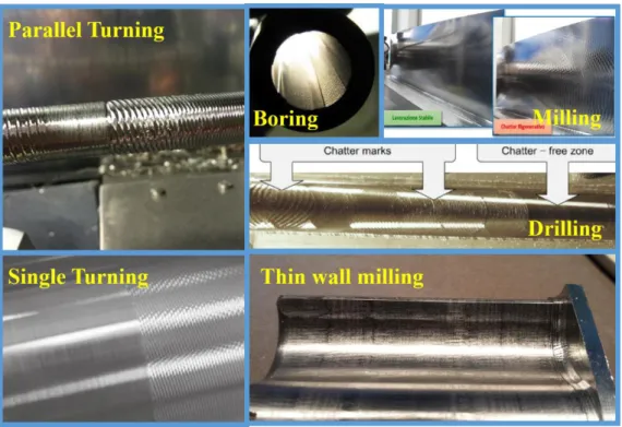
Tool wear, cooling strategies, operating parameters (i.e. feed rate, spindle speed and depth of cuts), part measurements, various induced errors, components’ vibration and chatter instability, to mention but a few, are various factors that may contribute to the accuracy and productivity of the metal cutting techniques. Among them, that the chatter instability is considered as a most catastrophic threat to the part quality and process productivity is of no question which occurs in wide range of machining processes (see Figure 1.1).
2
Figure 1.1. Chatter instability in different cutting process
Cutting process which undergone chatter phenomenon are susceptible to poor surface finish, tool breakage, tool wear, inordinate operating noise, and henceforth; reduced accuracy and productivity. In early years of twentieth century, to Fredrick Taylor, chatter was a strange phenomenon under which impede the operator to face the problem owing to unidentified nature of the process [1]. After preliminary observation of Taylor, almost half a century later, Tlusty and polacek [2] and Tobias and Fishwick [3], independently, identified regenerative chatter as the main source of chatter instability. In fact, Tlusty [4], identified mode coupling as another source for chatter stability where there is a vibration with identical natural frequency and phase in the plane of the motion, i.e. two directions. Nonetheless, it is well-known that regenerative chatter initiate instability earlier than mode coupling [4], and thus it has been in the center of researchers’ interest.
3
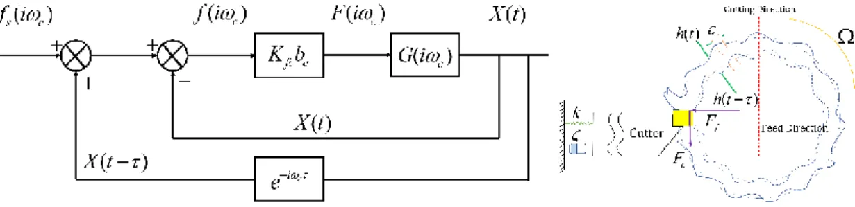
Figure 1.2. Regenerative chatter in an orthogonal turning operation
Oscillating tool leaves waves on workpiece’s surface due to vibrations which influence the chip thickness. In the next revolution, by and large, if the width of cut is big enough, the oscillating wave’s amplitude and its corresponding cutting force may increase. Successive increases in dynamic chip thickness and force called “regenerative chatter”. Regenerative chatter can be simulated in a simple closed-loop block diagram as illustrated by Figure 1.2.
In Tlusty’s and Polacek’s [2] chatter stability theory, stable depth of cut can be determined for given dynamic properties of cutter and the workpiece in addition to cutting force coefficient for a simple but a practical orthogonal turning process. Merrit [6] provided similar results for orthogonal turning operation employing Nyquist stability criterion. However, applying previous models was not able to predict the chatter stability in milling operations due to time-dependent and intermittent nature of the process. An approximate model to predict chatter behavior in milling process was introduced by Tlusty [7] by considering average number of cutting flutes and also directional factor to reduce the problem to a time-invariant problem. Later on, Tlusty [8–10], developed a time domain model to simulate the chatter instability in milling operation. Minis [11-12], presented a novel formulation for dynamic modelling of a milling operation utilizing the Floquet’s theorem and Fourier series expansion, and determine the stability limit based on Nyquist’s stability criterion. Altintas and Budak [13], also presented an analytical model for predicating the chatter stability in milling process. In their model, time-varying behavior of the process is approximated with ZOA method in which only considers the constant coefficient in the Fourier series expansion of the directional factor to transform it to a time-independent problem. Even though, their method turned to be very time-efficient in constructing stability maps, the accurate results were only limited to high immersion conditions and/or high number of teeth. To improve the predictions, Budak [14-15]
4
developed a multi-frequency solution to the chatter stability modelling of the milling operation which consider higher number of harmonic frequency and consequently succeeded to predict the chatter instability in low immersion conditions.
Regardless of numerous investigation of chatter instability so far, chatter will remain as a crucial problem in the future of machining industry due to the several factors as listed below [5]:
• Demand for increase in Material Removal Rate (MRR)
• Limitation of machine tool manufacturer in designing well-damped structures1 • Inclination toward utilizing low friction guiding systems which are weakly
damped
• Tendency to produce light-weight machine tools make them to be susceptible to unwanted vibration
• Flexible part machining
Nonetheless, since the identification of self-excited chatter instability, researchers and engineers had sought for procedures to suppress its unwanted vibration and therefore; eliminate the repercussion accompanied by the process. Some of these techniques are briefly mentioned in the next.
Stability Lobe Diagrams (SLD) are generated to avoid chatter instability by proper selection of process parameters, i.e. time delay (spindle speed since 𝜏 = 60/Ω) and depth of cut. Stability diagrams can be constructed for a machine tool structure with known dynamic properties, cutter geometry, force coefficient and process parameters. Figure 1.3 shows a common stability lobe diagram on a machine tool for a specific cutting process. As can be observed in Figure 1.3, system can be stable or unstable for each pair of spindle speed and depth of cut. Those combinations of the spindle speed and axial depth of cut lower than the limiting boundaries result in stable operation, whereas those points located in the upper parts leads to instable processes. Constructing such diagrams before initiating a cutting process help the machinist to select a proper spindle speed-depth of cut pair to
1 FEM is able to predict natural frequencies and mode shapes of the machine tool components in early
stages of designs. However, it may lead to false predictions when it comes to calculation of the damping properties of the structures. Such discrepancies mainly root in limitation of FEM in modelling of the joints as the main source of dissipating the energy [4].
5
avoid chatter. Obviously, seeking for a stable process by trial and error procedure would be a time and energy consuming process.
Figure 1.3. A common Stability Lobe Diagram (SLD) [5]
Spindle speed variation is an attenuating technique based on varying chatter wave modulation which are reasons behind instabilities [16]. In addition to spindle speed which can reduce regenerative chatter by varying the time delay in the process, variable pitch cutters can be utilized to intervene in time delay between chatter waves and improve stability [17-18]. Process damping, as well, can significantly hamper the disastrous effects of chatter instability in relatively low chatter frequencies and low spindle speeds [19-20]. Moreover, passive (TMDs2 [21]) and active (Active tools [22], Active fixtures [23]) vibration absorber can effectively enhance the damping of the structure and result in stable processes. Recently, the idea of parallel machining has been conceived not only because of its favorable MRR, but also because of its ability to suppress chatter vibration during flexible part machining.
Since in this thesis the focus is on the parallel machining operations, general aspects of the such processes will be further elaborated in the next.
Parallel machining has received considerable attention in various manufacturing industries owing to their advantageous compared with traditional single operations. Clearly, employing extra cutting tools simultaneously will increase the material removal rate and obviously the productivity of the parallel processes. Furthermore, additional process and geometry parameters may be tuned for enhanced stability in simultaneous turning. For instance, utilizing two cutters with 180 degrees of difference in radial direction may results in cancelling the forces acting on the workpiece, and thus
6
suppressing the chatter vibration. Moreover, radial angle between the cutters, for example, can be selected in a way to modify the dynamic chip thickness modulation for enhanced stability. Also, dynamics of the different components can be tuned to reduce the chatter vibration during the parallel machining. Similarly, extra process geometry while parallel turning, i.e. nose radius, inclination angle, rake angle and side edge cutting angle of the insert, can effectively be selected to observe the best stability behavior. And finally, different configuration of the components, i.e. cutters and workpiece, respect to each other, provide ability to perform various types of operation at the same time. Neither of aforementioned parameters can be modified in conventional turning which make the parallel turning pioneer to their traditional counterparts. Nevertheless, dynamics and chatter stability analysis of a simultaneous turning operation become further complicated because of the presence of various dynamic interactions between different components of the system in comparison with conventional turning operation. In case of a relatively rigid workpiece, the cutters may be coupled via the structure (turret and tool holder) or shared cutting surface. Intuitively, if neither of previous coupling scenarios exist, tools perform single mode turning operation with no coupling. It should be noted that during cutting a flexible workpiece, in addition to coupling through the shared surface or structure of the turret, components are coupled via the workpiece structure. Given above information, it is essential to have a comprehensive perspective over the dynamic and geometrical modelling of parallel turning operation in order to ensure a stable process by appropriate selection of process and geometry parameters.
1.1 Literature Survey
Chatter instability may results in jeopardizing enhanced productivity in parallel turning operations [24-25]. However, parallel machining can be employed as a chatter suppression technique in machining of flexible workpieces [5] and machining with flexible tools [25-26]. In parallel turning of a flexible workpiece, not only the tools’ dynamics and their dynamic interaction but also the dynamics of the workpiece are crucial factors in stability analysis of the process. Consequently, ensuring a chatter-free cutting condition requires an appropriate selection of process parameters and process geometry which is achievable by having a precise and comprehensive insight into the modeling of the process geometry and dynamics. Even though, the number of publications on the one-dimensional chatter stability analysis is considerably high and go back to almost half a
7
century ago [2-3], there are few authors who investigated a general model for stability analysis of turning operations. Rao [27] developed an analysis in which the nose radii and cross-coupling effects between radial and axial displacement, in addition to sensitivity of the cutting force coefficients to smaller chip thicknesses has been taken into account. Later, Ozlu and Budak [28] presented an analytical multi-dimensional model to predict the stability limits in turning and boring processes. Their model considers all major parameters of the process geometry such as oblique angle, approach angle and nose radius, and more importantly the dynamic effects of tool and workpiece in different directions. Results in [28] shows that true geometry of the insert plays a vital role in the chatter stability of flexible part turning. In fact, by increasing the nose radii and side edge cutting angle of the insert absolute chatter stability of the process decrease drastically. Nonetheless, until recently, dynamics and stability of parallel turning operation has not been investigated extensively. Lazoglu [29] proposed a time-domain approach to stability of parallel turning system with two tools which are clamped on different turrets and cut different surfaces. The model includes the effect of both the tools’ and the workpiece’s dynamics. They demonstrated that for relatively flexible workpiece system, the stability limit in a conventional turning operation is slightly higher than the parallel process limit. Ozdoganlar and Enders [30] proposed a stability model for parallel turning operation of a symmetric system and verified their results through the experiments. Ozturk and Budak [25] proposed both frequency and time domain models for the stability of an orthogonal multi-delay parallel turning operation. In their model, the tools were coupled through the shared surface while each of the tools was cutting different depth of cuts. Results demonstrate that stability limit could increase according to the dynamic interaction between the tools creating an absorber effect. The results in [25] indicates MRR can be enhanced not only by exploiting extra cutting edges but also by proper selecting the process parameters. Brecher et al. [26] investigated the parallel turning operation in which cutters removed the same depth of cut from the workpiece considering various dynamic coupling of the tools through the machine structure. Frequency and time domain approaches supported that the radial angle between the tools has remarkable effects on shifting the stable depth of cut for the dynamically coupled tools [26]. In contrast, no significant dependence of the chatter stability limit to the radial angle were observed while using tools with independent dynamics transfer functions. Ozturk et al. [31] used two different cutting strategies in parallel turning, i.e. cutters cutting a shared surface of the rigid workpiece and cutters clamped on a turret removing material from different
8
surfaces of a rigid workpiece. Moreover, Ozturk et al. [31] for the first time emphasized the prominent influence of natural frequency ratio of the tools in chatter stability of parallel turning operations. They demonstrated that by adding or removing mass, and changing the tool holder’s length, the system can be tuned for enhanced productivity. The results denoted that dynamically identical tools give the worst stability limit. Similarly, Reith at el.[32-33], theoretically and experimentally scrutinized the effect of tuning natural frequency of the tools and dynamic vibration absorbing potential on the stability of parallel turning operation. They have confirmed that using detuned cutters in parallel turning the MRR can be increased by shifting the stability boundaries upwards. Recently, Reith et al. [34] utilized non-proportional damping to model the multi-cutter system which includes the dynamic coupling between the cutters via the fixture. Their results showed that presence of non-proportional damping further improves the stable boundaries of a detuned cutter system. Although several works have been reported mainly focusing on 1D dynamic modeling of chatter stability for parallel turning operations and tuning the process to suppress chatter instability, multi-dimensional chatter stability considering true geometry of cutting tool and workpiece dynamics for different parallel turning strategies has not been investigated so far.
1.2. Objectives
The primary objective of this study is to develop a general multi-dimensional stability model for different parallel turning strategies. Two main strategies where tools can cut the workpiece’s surface, i.e. cutting a shared surface, or cutting different surfaces are presented. For the first time in modeling of parallel turning, main parameters of process geometry, i.e. side edge cutting angle and nose radii of the tools, are included in the analysis. Moreover, tool and workpiece dynamic compliance effects are accounted for in the model to improve the stability limit predictions. Frequency and time domain stability models are developed for parallel turning strategies where effects of process parameters on the chatter behavior are thoroughly investigated. Simulation predictions are compared and verified with the experimental results. Finally, for each parallel turning strategy, best process parameters for a stability-guaranteed and productivity-enhanced operation is identified.
9 1.3. Organization of the Thesis
The thesis is outlined as follows:
• In chapter two, configurability in parallel turning process is emphasized as an advantageous of the process compared with their conventional counterparts. Two different strategies (of interest) in parallel turning operation has been introduced. Different dynamic coupling scenarios for each strategy is elaborated. Finally, practical limitation or advantageous of each strategy has been magnified.
• In chapter three, a multi-dimensional chatter stability model is presented for introduced strategies in chapter two. Workpiece and cutter’s flexibility is accounted for in developing the formulations. Additionally, true geometry of the inserts is considered. After deriving the eigenvalue problem, a numerical MDBM is utilized to solve the equation in the frequency domain. To have a better insight into the chatter phenomena and its initiation, a time domain model is constructed in MATLAB/Simulink based on the chip thickness definition.
• In chapter four, simulated results of frequency and time domain model is compared with the experimental results. Stability maps for each parallel turning strategy and flexibility scenarios (four cases in total) is generated and good agreement is observed with test results. Effect of cutters’ depth of cut in addition to inserts’ geometry parameter’s is investigated on the stability maps. Provided stability map in the current thesis give the operator a good insight over the parameter selection in parallel turning operation to gain a stable process where was performed as a trial and error procedure previously.
• In chapter five, the summary of the thesis is presented along with major conclusion of the thesis.
10
DIFFERENT STRATEGIES IN PARALLEL TURNING OPERATIONS
Configurability is another advantage of parallel turning operations. Although increased process and geometry parameters in addition to dynamic interactions among the components may hamper controlling the chatter instability, adjusting proper cutting conditions in each configuration can be advantageous for attenuating the chatter vibrations. In the following, two main strategies used in this study is presented.
2.1. Cutters on Different Turrets Cutting a Shared Surface
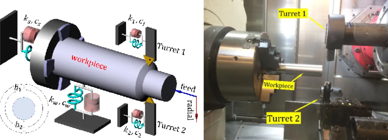
Figure 2.1 demonstrates a schematic illustration of a parallel turning operation in which cutters mounted on different turrets machine a shared surface of the workpiece. As can be observed in Figure 2.1, dynamic contribution of different components, i.e. the cutters, the workpiece and the spindle structure, has been considered.
Figure 2.1. Cutters mounted on different turrets cutting a shared surface (coupled via the shared surface
Generally, given geometry of most of turning operations, tools are considered to be flexible in the feed direction while workpieces are considered to be flexible in the radial
11
direction. However, in current study, a general formulation is presented in which dynamic effect of the cutters in radial direction, in addition to dynamic effects of the workpiece in the feed direction can be easily taken into account. It is noteworthy that various components in the process can experience different coupling scenarios. During cutting a relatively rigid workpiece by flexible cutters, cutters do not have any dynamic coupling through the structures. In fact, dynamic forces acting on one of the cutters cannot influence the dynamic force of the another one. However, in this configuration, even though the tools are not dynamically coupled via the, waviness on the surface due to vibrations of one of the tools causes variation of the chip thickness on the other tool; hence, tools are dynamically dependent. While cutting the shared surface of a flexible workpiece, on the other hand, in addition to dynamic coupling of the cutters via the shared surface, the cutters are coupled via the workpiece as well. As a matter of fact, radial dynamic forces acting upon on one of the cutters can affect the radial dynamic force applied on the other one owing to dynamic cross transfer function created by radial flexibility of the workpiece.
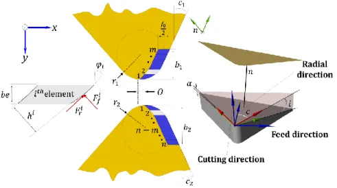
Figure 2.2. Modulated chip thickness on the tools having nose radius (r) and side edge cutting angle (C). A 3D view of the cutting insert. 𝑖, 𝛼 𝑎𝑛𝑑 𝑐 are inclination, rake and side edge cutting angle, respectively. Elemental forces acting on an ith element located
on the cutting edge of an insert.
In this configuration, feed velocity of the cutters must be the same. In addition to the identical feed velocity of the cutters, axial offset between the cutters should be equal to 𝛰 = (𝑏2−𝑏1)×𝑡𝑎𝑛𝐶 to make sure that cutting surface is shared and distributed equally over the tools, where 𝑏2 and 𝑏1 are depth of cuts for the second and the first cutters, respectively, and 𝐶 is side edge cutting angle of the insert (see Figure 2.2). The axial
12
offset between the tools must be kept in the range of 𝛰 ± 𝑓0⁄2 not to violate the parallel cutting condition [25] where 𝑓0 is feed velocity of the tools.
During cutting with tools having different side edge cutting angles, the cutting surface cannot be shared equally over the tools, and thus parallel operation condition cannot be met. Consequently, tools with different side edge cutting angle are not employed in this configuration. It is worth noticing that tools can cut a shared surface with different or identical depth of cuts. As will be further discussed in Chapter 3,parallel turning having tools with different depth of cuts is considered as a double-delay system while on the contrary, parallel turning with tools having similar depth of cut is a single-delay system.
2.2. Cutters cutting different surfaces
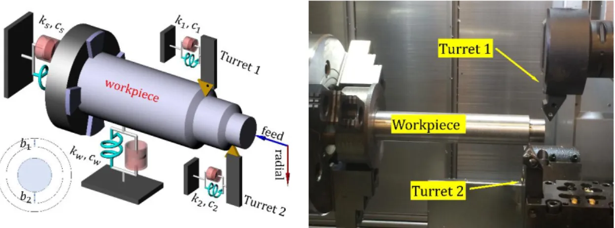
Another parallel turning operation in which two tools cut different surfaces is illustrated in Figure 2.3 and Figure 2.4. wherethe cutters can be mounted on different turrets or on the same one. There is no coupling between the cutters through the surfaces, however cutters can be coupled via structures, i.e. turret or workpiece.
Figure 2.3. Cutters mounted on different turrets cutting different surfaces (Coupled via the workpiece dynamics)
To elaborate, during machining of a flexible workpiece with rigid tools, the only dynamic coupling between the cutters occurs due to the flexibility of the workpiece in the radial direction. Nonetheless, while machining a rigid workpiece with flexible tools which are installed on a single turret, dynamic coupling among the cutters is owing to the flexibility of the turret/tool holders structure in the radial direction.
13
Figure 2.4. Cutters mounted on the same turret cutting different surfaces [31] (Coupled via the turret structure)
Similar to the previous case, tools can have different or identical depth of cuts. Feed velocity of the cutters is set to be the same. However, unlike the previous case, tools having different side edge cutting angles can be utilized, and thus this additional geometry parameter can be adjusted properly for enhanced productivity.
In addition to mentioned configurations, there is two different types of tools/workpiece combination in the literature. Brecher et al. [26] (see Figure 2.5 ), investigated a parallel turning operation in which cutters can have radial alignment respect to each other. The results indicate that radial orientation of the tools when they are dynamically coupled, has prominent influence on increasing the chip removal rate. Hence, in addition to selecting spindle speed, radial angle between the cutters can be tuned to increase the productivity. Also. Reith et al. [32], developed an analytical formulation to chatter stability of a parallel turning having arbitrary number of cutters (see Figure 2.6). Despite the strong theoretical framework of the work presented in [32], to the author’s knowledge, it is hard to implement the multi-cutter configuration in the industry since setting up the fixture seems to be complicated and it may rise obstacles to the machine operator to tune the cutters.
14
Figure 2.5. Dynamic coupling between the cutters and influence of radial angle on the delay between the cutters [26]
15
DYNAMIC MODELLING AND PROCESS STABILITY
A multi-dimensional model is presented and applied to two introduced configurations. 3.1.1. Dynamic Chip Thickness
In contrast with previously developed models for parallel turning [25-26], [29-35], the current study considers effects of side edge angle and nose radius in different parallel turning strategies. To describe the chip geometry of an insert in the nose region, the area must be divided into smaller trapezoid-like elements [28], as illustrated by Figure 2.2. Geometrical parameters describing each element in the nose region, i.e. the elemental depth of cut (𝑏𝑒) and side edge cutting angle of each element (𝜑𝑖) were introduced in [28]. The modulated chip thickness and forces parallel and perpendicular to the cutting edge of the element must be projected in the global coordinates of the CNC machine. As far as cutting depth on each tool is different, two different regions describe the cutting process. In the first region, the depth of b1 is removed by the first and second tools simultaneously.
In the second region, on the other hand, the cutting depth of b2-b1 is solely cut by the
second tool. In each of these regions a different time delay exists, presenting a double-delay system. In the former region, the vibrating cutting edge of a tool removes the surface generated by the other tool at a half rotation period before. Thus, the delay in this region is equal to 𝜏/2. Moreover, the static part of the chip thickness which is shared evenly between the cutters is equal to feed per revolution. Then, the total chip thickness for each element on the tool can be written as a summation of regenerative and static parts of the chip thickness as follows:
1 1 1 2 2 2 1 12 , 12 , 2 21 , 21 ,cos sin cos , 1,
2
cos sin cos , ,
2 i s c i c i c j s j c j c c f h t C y x i m f h t C y x j n m n (1)
where ∆𝑥12 and ∆𝑦12 are given by:
1 2 1 2 12 12 2 2 2 2 c c w w c c w w y y t y t y t y t x x t x t x t x t (2)16
where ∆𝑥21 and ∆𝑦21can be defined similarly. In the latter region, however, vibrating edge of the second tool cuts the surface left by the same tool from one revolution before, and thus the delay in this region is equal to 𝜏. Furthermore, the static part of the chip thickness is equal to the feed per revolution. Therefore, the total chip thickness in the second region can be expressed as follows:
2 22 cos 2 22sin , 22cos , , 1, 1
j s j c j c c h t f C y x j n m (3) where:
2
2
2 2 22 22 c c w w c c w w y y t y t y t y t x x t x t x t x t (4)Although, one may consider the dynamic vibration of the cutters or the workpiece in either positive or negative direction, dynamic chip thickness definition must remain unchanged. For example, based on the coordinate system shown in the Figure 2.2, the current dynamic displacement of the first cutter in the positive 𝑥 direction increases the chip thickness of the first tool while dynamic displacement of the second tool at half revelation before in positive 𝑥 direction decreases the chip thickness of the first tool. Same rule should be applied to form the dynamic chip thickness.
In equations (1-4), 𝑦 and 𝑥 represent the cutter and workpiece displacements in radial and feed directions, respectively. 𝑡 and 𝜏 are time and period of rotation, respectively. Furthermore, 𝑓𝑠 and 𝐶 are the feed per revolution and side edge angle of the cutting tool, respectively. Finally, n and m are the number of elements used in meshing of the second and the first tool, respectively. As aforementioned, if the cutting depths on each tool are identical, the only delay in the process is 𝜏/2, the parallel turning operation is a single-delay system. In this case, the dynamic chip thickness on each of the tools can be presented as follows:
1 1 1 2 2 2 1 12 , 12 , 2 21 , 21 ,cos sin cos , 1,
2
cos sin cos , 1,
2 i s c i c i c j s j c j c c f h t C y x i m f h t C y x j m (5)
17
1 2 1 2 12 12 2 2 2 2 c c w w c c w w y y t y t y t y t x x t x t x t x t (6)where ∆𝑥21 and ∆𝑦21can be defined similarly.
3.1.2. Dynamic Cutting Forces
By summing the transformed forces acting on each element on the cutting edge of the insert, the total forces in feed and radial direction, F Fx, y, can be calculated as follows:
1 1 1 1 1 2 2 2 2 1 2 2 2 2 12 1 12 1 22 21 1 22 21 [ ][ ][ ] [ ][ ][ ] [ ][ ][ ] m x i i e c c c i y c n m n x j j j j e c c c e c c c j j n m y c F x b T C D y F F x x b T C D b T C D y y F
(7)where [𝐷𝑐𝑖1] and [𝐷𝑐𝑗2] project the chip thickness onto the global coordinates, [𝐶𝑐1]and [𝐶𝑐2] represent the force coefficient matrix and 𝑏𝑒is the width of each element. Matrices [𝑇𝑐𝑖1] and [𝑇𝑐𝑗2] transform the forces acting upon the cutting edges onto the feed and radial directions.
3.1.3. Stability Analysis using Frequency Domain Solution
Dynamic displacements of the system,
x y
p,
p, can be determined by using dynamic cutting forces, Fxp,Fyp, and dynamic transfer functions as follows [13]:1 2 ( ) ( ) , : , , ( ) ( ) p p p p xx xy x p p p yx yy p y x t G G F t p c c w G G y t F t (8)
It should be noted that considering the geometry of most turning processes the tools can be assumed to be flexible in the feed direction whilst the workpiece is flexible in the radial direction only. Hence, cross transfer functions can be neglected in the calculations. Marginal stability is obtained when the real part of the characteristic equation is zero and the system oscillates with a constant amplitude at the chatter frequency of 𝜔𝑐 [36]. Therefore, the dynamic displacements and forces can be expressed as follows:
18
, ,
, : , ,1 2 c c i t p p i t x y x y p x y e G F e p c c w (9)Equation (9) represents six equations for the displacements of cutter 1, cutter 2 and workpiece in the feed and radial directions. However, since it is assumed that cutters never lose their contact with workpiece, equations pertaining to the workpiece’s displacements can be written in terms of cutters’ displacement as follows [15]:
1 2 1 2 c c c c i t w c c i t w xx x x i t w c c i t w yy y y x e G F F e y e G F F e (10)Substituting equations (9-10) in equation (7), and re-arranging them in a single matrix form [15], the global dynamic force matrix becomes:
1 2
1 1 1 1 1 2 1 2 2 2 2 2 ( , ) ( , ) ( , ) ( , ) c c c c x x c c y i t y i t e c e c c c x x c c y y F F F F e b A m n G i b A m n G i e F F F F (11)Matrices in equation (11) are as follows:
1 1 1 2 2 2 2 2 2 2 2 1 1 2 2 2 2 2 2 1 2 2 2 1 [ ][ ][ ] [0 ] ( , ) , [0 ] [ ][ ][ ] [0 ] [0 ] ( , ) [0 ] [ ][ ][ ] m i i c c c i n j j c c c j n m n m j j c c c j T C D A m n T C D A m n T C D
(11-1) Also 1 2 1 2 1 2 1 2 2 2 1 2 2 0 0 0 0 0 0 0 0 c c c c i c w c w xx xx xx xx i c w c w yy yy yy yy i c w c w xx xx xx xx i c w c w yy yy yy yy G G R G e G R G G R G e G R G G e G R G G R G e G R G G R (11-2) and19 2 2 0 0 0 0 0 0 0 0 0 0 0 0 w c w xx xx xx w w yy yy G G R G R G R G R G R (11-3) where 𝑅 = 1 − 𝑒−𝑖𝜔𝑐𝜏 2⁄ , 𝑅′= 1 − 𝑒−𝑖𝜔𝑐𝜏.
Equation (11) has nontrivial solution if the determinant of the following characteristic equation is zero:
1 1 2 2
4 4 1 2
det e ( , ) ( c, ) e ( , ) ( c, ) 0
E I b A m n G i b A m n G i (12) where 𝐼 is the 4×4 identity matrix. Since Equation (12) is a complex one its real and imaginary parts must be set to zero:
11
R{ , , , , } 0 { , , , , } 0 e c e c E b m n I E b m n (13)where Ω = 60 𝜏⁄ is the spindle rotation period. For the current configuration, before proceeding to the stability calculations, three parameters must be chosen initially. Firstly, depth of cut of the second tool, (b2), and secondly, the number of elements which mesh
the nose region of the first and second cutter, (mnose, nnose), respectively. For the sake of
simplicity, mnose and nnose are selected in a way that the depth of each element for both
tools is equal, i.e. 𝑏𝑒1 = 𝑏𝑒2. As the next step, the total number of elements in the second tool, i.e. n=b2/𝑏𝑒1, can be determined. Finally, the number of elements which are in cut
on the first tool, i.e. m, can be calculated by solving the eigenvalue problem iteratively. Multi-Dimensional Bisection Method (MDBM) [37-38], provides a fast and efficient algorithm to locate the roots of Equation (13). Similar with proposed solution in [28], it should be noted that the presented solution (see Equations. (12) and (13)) determines the elemental stability limit, (be_stable), which is the stability limit of an element in the cutting
edge of the first tool. Hence, the total stability limit of the tool should be computed by multiplying the number of elements in the cut by the elemental stability limit, i.e. m×be_stable. In order to achieve the elemental stability limit using MDBM, firstly, an
appropriate range and incremental step for the chatter frequency, 𝜔𝑐, spindle speed, Ω, and elemental depth of cut, 𝓌, must be selected. Matrices 𝐴̅̅̅1 and 𝐴̅̅̅2 are calculated for one element engagement of the first cutter. Later, the elemental stability limit is computed
20
by solving equation (13). In the next step, it should be checked if calculated stability limit (m×be_stable) is inside the part of the cutter edge considered in the calculation of eigenvalue
problem.
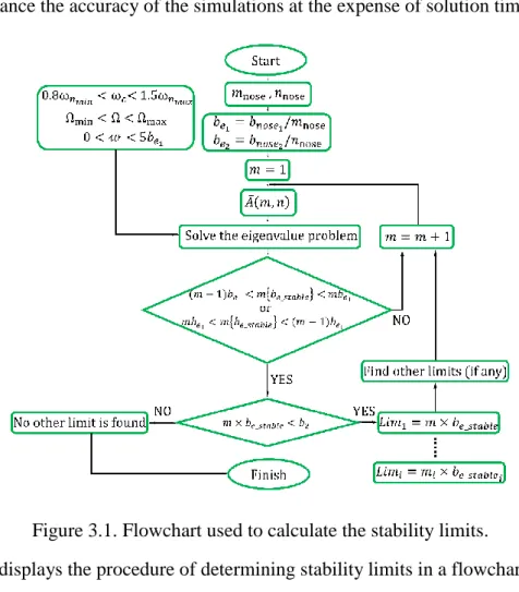
1 1 1 1 _ _ 1 1 e e stable e e e stable e m b m b mb mb m b m b (14)If condition stated in Equation (14) is not met, another element will be added and the same procedure will be repeated until the determined stability limit satisfied equation (14). It should be noted that large number of meshes in the nose region of the tools will further enhance the accuracy of the simulations at the expense of solution time.
Figure 3.1. Flowchart used to calculate the stability limits.
Figure 3.1 displays the procedure of determining stability limits in a flowchart. In the formulations, it is assumed that b2 is equal and bigger than b1, and thus those 𝑏1 values which are smaller than 𝑏2 are acceptable solutions. However, to complete the stability map for 𝑏1 > 𝑏2 values, tools’ or workpiece contact points’ dynamics must be swapped in the simulations and then calculated 𝑏2 for given 𝑏1 can be plotted in the same map.
21 3.1.4. Time Domain Model
Created forces during cutting process will cause vibrating the tools and workpiece. Subsequently, the modulated dynamic chip thickness of the tools will be influenced by the dynamic properties of the system. Since the cutting forces depend on dynamic chip thickness, modulated chip thickness in current revolution of cut will be affecting the cutting forces in the next revolution. The governing delayed differential equation (DDE) of the system can be modeled (see Figure 3.2) in MATLAB/Simulink [39] as a closed loop block diagram [26], [35-36]. Even though inclusion of the static chip thickness and edge forces in the time domain model will not influence the stability boundaries, it leads to predict accurate force and displacement values in the simulations. It is worth noticing that step size must be selected small enough in order to have sufficient simulation points in each chatter wave [25]. Runga-Kutta method [40] was used to solve the DDE.
Figure 3.2. Time domain block diagram to simulate the dynamic chip thickness of the first cutter.
In order to illustrate the time domain approach, dynamic displacements of the first cutter in the feed direction, which depend on dynamic displacement of second cutter and workpiece in both radial and feed directions, calculated in the Simulink environment and are given in Figure 3.2. The same procedure must be applied to determine the dynamic displacements of other components, i.e. cutter 1, 2 and the workpiece, in the
22
radial and feed directions. Thereafter, the displacements and delayed displacements must be feedbacked to corresponding block diagrams (∆𝑥12, ∆𝑦12, ∆𝑥21, ∆𝑦21) in accord with the definition of the dynamic chip thickness (see Equations (1-4)).
3.2. Two Cutters Cutting Different Surfaces
Another parallel turning operation in which two tools cut different surfaces has been illustrated in Figure 3.3. The cutters can be mounted on different turrets or can be mounted on a single turret. In this configuration in which one of the tool is performing roughing and the other one finishing operation is widely being used in industry. In case the tools are cutting different surfaces, similar with the first case, feed velocity of the cutters set to be the same. Nevertheless, in contrast with the first case, tools having different side edge cutting angles could be utilized. To develop stability formulation, same procedure as it discussed in the first case should be followed.
(a) (b)
Figure 3.3. Tool cutting different surfaces, (a) on different turrets, (b) on the same turret
The total chip thickness for the cutters are given by:
1 2 1 11 11 2 22 22
cos sin cos , 1,
cos sin cos , 1,
i c s i i j s j j c h t f k y x i m h t f k y x j n (15) Where:
23
1 1 1 1 1 1 1 1 2 2 2 2 2 2 2 2 11 11 22 22 c c w w c c w w c c w w c c w w y y t y t y t y t x x t x t x t x t y y t y t y t y t x x t x t x t x t (16)Indices 1 and 2 shows the contact points of the cutters. Similar with previous case formulation, total dynamic forces exerting on the tools in the general coordinate should be expressed in terms of dynamic transfer functions and dynamic displacement of the system’s component. By employing the extracted equations, and manipulating them algebraically to transform into a single matrix form, the following is obtained:
1 1 1 1 2 2 2 2 ( , ) ( , ) c c c c x x c c y i t y i t c c c x x c c y y F F F F e A m n G i e F F F F (17) Where 1 1 1 2 2 2 2 2 1 2 2 1 [ ][ ][ ] [0 ] ( , ) [0 ] [ ][ ][ ] m i i c c c i n j j c c c j T C D A m n T C D
(18) and
1,1 1,1 2,1 2,1 1 1 1,1 1,1 2,1 2,1 1 1 1,2 1,2 2,2 2,2 2 2 1,2 1,2 2,1 2,1 2 2 1 0 0 0 0 0 0 0 0 c w c w e xx xx e xx xx w c w c e yy yy e yy yy c w c w e xx xx e xx xx w c w c e yy yy e yy yy b G G b G G b G G b G G G b G G b G G b G G b G G (19)The equation 17 has nontrivial solution if the determinant of the following equation is zero:
4 4 det 1 i c ( , ) ( , ) 0 c E I e A m n G i (20)The solution method will be the same as the first case. Moreover, time domain simulation can be easily adapted from the first case diagrams, in accord with definition provided dynamic chip thickness for second case.
24
SIMULATIONS AND EXPERIMENTAL RESULTS
In order to discuss the chatter stability solutions of parallel turning obtained from frequency and time domain simulations, two different configurations with flexible tools and workpiece combinations (four cases in total) are investigated and verified experimentally. Modal parameter were derived from fitted curves to tap testing results [36] (Figure 4.1). In experiments, sound spectrum was measured and image of surface was taken in order to detect chatter. The force coefficients were calibrated mechanistically based on linear edge force model [41]. In each case, effects of the nose radius and the side edge cutting angle of the inserts on the stability are investigated and a methodology for proper selection of the process parameters is presented to enhance productivity in each configuration. The simulation and experimental results proved that by setting the depth of cuts of the tools in the parallel turning mode bellow the tools’ critical depth in single turning mode a chatter-free process can be achieved. However, the maximum stable MRR in each case can happen on different points of the stability map.
4.1. Cutting a Shared Surface 4.1.1. Flexible Workpiece
This set of experiments is conducted to observe the chatter stability of a parallel turning operation while cutting a shared surface of a flexible workpiece. Tools are clamped in a way to achieve the maximum stiffness in the feed direction. The workpiece and insert properties are given in Table 1. The workpiece was machined by SECO TNMG TP2501 inserts on a Mori Seiki NT CNC machine.
25
Table 1. Workpiece and process and geometry parameters [case 1]
Workpiece material AISI 1050 Feed cutting force Coefficient 𝐾𝑓𝑐 692 MPa Workpiece diameter 42 mm Feed edge force Coefficient 𝐾𝑓𝑒 148 N/mm Workpiece length 127 mm Radial cutting force Coefficient 𝐾𝑟𝑐 178 MPa nose radius 𝑟 0.4 mm Radial edge force Coefficient 𝐾𝑟𝑒 18 N/mm
side edge angle 𝐶 30° Feed velocity 𝑓0 0.1 mm/rev
inclination angle 5° Spindle speed Ω 1550 RPM
(a) (b)
Figure 4.1. Tap testing measurement and CutPro [36] (a). Parallel turning operation(b)
A major problem in chatter tests involving a flexible workpiece is its varying dynamic properties. In order to minimize the effect of dynamic properties variation, the cut length, i.e. the part where the diameter is reduced, is kept very short in comparison with the total length of the workpiece. Additionally, two identical workpieces were used to complete the stability tests. This was verified by the measured modal data of the workpiece which showed negligible variation before and after the cut. Modal data of the workpiece before and after the cut is presented in Table 2
26
Table 2, Modal data of the workpiece [case 1]
Component fn(Hz) Stiffness(N/m) Damping (%)
Workpiece (Before Cut) 538 1.2×10⁷ 1.7
Workpiece (After Cut) 575 1.28×10⁷ 1.52
Tool 1 3434 1.45×10⁹ 0.7
Tool 2 4020 1.93×10⁸ 2.29
Stability map for this case is generated by both frequency and time domain simulations, and verified experimentally as shown in Figure 4.2.a. The absolute stability limit of the tools for single tool operation mode is calculated as 0.84 mm using the model presented in [28]. The stability boundaries in parallel turning of a flexible workpiece forms an area separating the stable and unstable points for different depth of cuts. In a parallel operation, if the depth of cut of each tool is smaller than the stability limit of the same tool in the single tool operation, an individual upper limit for stable region exists since the lower stable limit is zero. By setting higher depth of cut values than the critical limit of the single tool turning, lower limit of stability map becomes non-zero, and thus system is transformed into a new stability region having upper and lower stability limits. By increasing 𝑏2, lines of lower and upper stable limit for 𝑏1increase proportionally parallel with line 𝑏2 = 𝑏1. As it can be seen in Figure 4.2.a, the difference between the lower and upper stable limits for 𝑏1, when 𝑏2 is bigger than 0.84 mm is about 0.75 mm which is almost equal to the stability limit of the single tool turning. In fact, a stable process can be approached where difference between the cutters’ depth of cut is less than the stable depth of cut of the cutters in single tool turning. In plainer words, total required radial force to initiate chatter instability are equal in both parallel and single turning.
On the line 𝑏2 = 𝑏1, from theoretical stand point, the dynamic forces acting on the workpiece in the radial direction should have exactly the same magnitude due to the identical nose radii, force coefficients, tool dynamics and depth of cut, and thus cancelling each other in this direction. Furthermore, since both tools are assumed to be rigid, theoretically the stability limits reach infinity.
27
(a) (b) (c)
Figure 4.2. (a) Stability map predicted by frequency solution and time domain model at 1550 RPM. (b) Dynamic chip thickness for three different points at b2=1mm. (c) Chatter
marks left on the surface in stable and unstable processes.
In order to observe the stability behavior of the system experimentally, the second cutter’s depth of cut is set to 1mm, and for three b1 values (0.5,1 and 1.5 mm) dynamic
displacement of the workpiece is simulated in the time domain and illustrated in Figure 4.2.b. The generated surfaces after the tests for three different depths of cuts are shown in Figure 4.2.c. As it is clear from the time domain simulations and the resulting surfaces, point A and C are unstable cases whereas B is a stable one.
(a) (b) (c)
Figure 4.3. Frequency spectrums of the measured sound and dynamic displacements of the workpiece simulated in the time domain for points (a) A, (b) B and (c) C.
In Figure 4.3, the spectrums of the sound measured during the experiments for points A, B and C are compared with the spectrums of the simulated dynamic displacements of the workpiece in time domain. At point C, because of the material removal from the
28
workpiece, natural frequency increased slightly causing the chatter frequency to be higher than the one for point A.
Even though there are some differences between the simulation and experimental results, the overall trends are similar. The discrepancies may root in the difference between the force coefficients of the upper and lower tools. To elaborate, sensitivity of the stability limit to variation of cutting force coefficients is demonstrated by an example case illustrated in Figure 4.4. The force coefficients for two tools may not be exactly the same due to slight differences in insert or tool holder geometries resulting in different nose and edge hone radii as well as rake or inclination angles owing to manufacturing tolerances of these features. According to the calculated stability limit, point D and D’ in Figure 4.2.a lie within the stable area boundaries. However, in the experiments, point D found to be unstable. Figure 4.4 demonstrates the dynamic displacement of the workpiece, calculated in the time domain, for 50 revolutions for points D and D’ based on new sets of force coefficients. It can be seen from the figure that even less than 10 percent change in cutting force coefficients of the tools, can change a stable cut to an unstable one for relatively higher depth of cuts, i.e. point D, due to the higher unbalanced forces in the radial directions. However, point D’ still remains in the stable condition due to smaller depth of cut, and thus smaller unbalanced forces in the radial direction.
(a) (b)
Figure 4.4. Effect of 10% change in the force coefficient of the first tool (Kf1=760MPa, Kr1=196Mpa) on the stability limit. (a) Point D’ stable process, (b)
Point D unstable process.
In accord with the fact that radial forces are countering each other in parallel turning of the shared surface of a flexible workpiece, employing geometrically and mechanically identical cutters, will lead to improved productivity. Intuitively, in the current configuration, line 𝑏1 = 𝑏2 provide the maximum productivity.
![Figure 1.3. A common Stability Lobe Diagram (SLD) [5]](https://thumb-us.123doks.com/thumbv2/123dok_us/23303.3003565/19.892.246.680.197.405/figure-a-common-stability-lobe-diagram-sld.webp)
![Figure 2.4. Cutters mounted on the same turret cutting different surfaces [31]](https://thumb-us.123doks.com/thumbv2/123dok_us/23303.3003565/27.892.158.788.106.336/figure-cutters-mounted-turret-cutting-different-surfaces.webp)
![Figure 2.5. Dynamic coupling between the cutters and influence of radial angle on the delay between the cutters [26]](https://thumb-us.123doks.com/thumbv2/123dok_us/23303.3003565/28.892.158.786.104.355/figure-dynamic-coupling-cutters-influence-radial-angle-cutters.webp)