AUTOMATIC AND CONTINUOUS
PROJECTOR DISPLAY SURFACE CALIBRATION
USING EVERY-DAY IMAGERY
Ruigang Yang and Greg Welch
The Office of the Future Project, Henry Fuchs, PI Department of Computer Science, CB# 3175
University of North Carolina at Chapel Hill Chapel Hill, NC, 27599, USA
{ryang, welch}@cs.unc.edu http://www.cs.unc.edu/{~ryang, ~welch}
ABSTRACT
Projector-based display systems have been used in computer graphics for about as long as the field has existed. While projector-based systems have many advantages, a significant disadvantage is the need to obtain and then adhere to an accurate analytical model of the mechanical setup, including the external parameters of the projectors, and an estimate of the display surface geometry. We introduce a new method for the latter—for continuous display surface autocalibration. Using a camera that observes the display surface, we match image features in whatever imagery is being projected, with the corresponding features that appear on the display surface, to continually refine an estimate for the display surface geometry. In effect we enjoy the high signal-to-noise ratio of "structured" light (without getting to choose the structure) and the unobtrusive nature of passive correlation-based methods. The approach is robust and accurate, and can be realized with commercial off-the-shelf components. The method can be used with a variety of projector-based displays, for scientific visualization, trade shows, entertainment, tele-immersion, or the Office of the Future. And although we do not demonstrate it in this paper, we have also been working on extending the method to include continual estimation of other system parameters that vary over time. CR Categories and Subject Descriptors: 1.4.1 [Image Processing and Computer Vision]:Digitization and Image CaptureImaging geometry; Scanning; 1.4.8 [Image Processing and Computer Vision]: Scene AnalysisRange data; Shape
Additional Keywords and Phrases: Computer Vision, Image Processing, Shape Recognition
1. INTRODUCTION
Technological and economic improvements are helping to make projector-based display systems increasingly a viable option for applications such as large-scale scientific visualization, simulation, or entertainment. Example systems include the CAVE™ [Curz93], the ReActor Room (and similar systems) by Trimensions, the Office of the Future [Raskar98], the Princeton Display Wall [Li00, Saman99], and the Stanford Information Mural [Humph99]. Beyond permanent fixtures, such display systems are often used for portable visualization, for example at conferences or trade shows. On a much larger scale, newer and more powerful light projectors are increasing opportunities to turn large physical structures into temporary projector display surfaces.
For example, during the millennium celebration in Egypt, the Pyramids were used as display surfaces for dynamic imagery.
While projector-based systems offer many advantages over other display options for many applications, a significant disadvantage is the need to obtain an accurate analytical model of the mechanical setup, including the external parameters of the projectors, and a description of the display surface. The problem is that the display surface is not an integral part of a single device, and therefore it must be initially characterized, and periodically monitored. We present an iterative approach to automatically determine the display surface geometry, without human intervention, unobtrusively and continuously while the system is being used for real work. We use
cameras in a closed-loop fashion to automate the process. Given the physical relationship between projector and a camera, and an initial (rough) estimate of the display surface geometry, we iteratively refine the estimate based on image-based correlation between the known projector image, and the observed camera image. Specifically we use a Kalman filter to estimate the length of a (parametric) ray from each projector pixel. The result is a complete 3D description of the surface, allowing one to modify the projected imagery so that it appears correct from any given viewpoint [Raskar99]. Some experiments results are shown in Figure 1.
It is interesting to consider the inherent appropriateness of this approach for display surfaces. Typically, finding feature correspondence using correlation techniques is less reliable for images or regions that lack high-frequency content. However, for our particular application, it is OK to miss measurement opportunities in such a region because if there are no problematic features for the system to observe, there are none for the human to observe either. When there are noticeably distorted features, the user will see them, but so will the system, which can then account for them by adjusting the estimate of the display surface. Given a sufficient variation of the projected image contents over time, the system eventually converges on the actual display surface geometry. Because our method is non-intrusive, the calibration process can always been running to maintain an optimal calibration while the system is being used for real work. Our simulation results (described later) predict a high degree of accuracy, and our actual implementation appears to agree. Our approach has the following key advantages:
! Self-calibrating. Once started, no human intervention is needed.
! Continuous and unobtrusive. Close-loop continuous calibration that does not affect the projected image quality. When there are visible problems it corrects them, when there are not, it does nothing.
! Robust. We use a Kalman Filter (minimum variance stochastic estimator) to optimally weight the measured correlation, with a relatively conservative tuning to reduce the likelihood of a negative impact from a false correlation.
! Minimal equipment. No need for high-speed cameras or projectors, or specialized image processing hardware
! Flexible setup. The cameras must be rigid but can be located relatively casually with respect to the projectors. The only restriction is that what they cannot “see” they cannot be used to calibrate.
! Stochastic framework. Because the framework is in place, other parameters can be added to the list of elements to be estimated. For example, internal projector parameters could be estimated using techniques similar to [Azarb95].
Our goal is to improve the setup and maintenance of conventional projector-based display systems, and to further enable the rendering of perspectively corrected imagery on more unusual surfaces [Raskar98, Raskar99].
2. BACKGROUND
One can categorize different calibration methods as passive vs. active, and online vs. off-line. Active methods usually inject energy into the environment to aid in the estimation of the surface properties, while passive methods use only existing energy in the environment. Off-line calibration methods are performed while the system is not being used, and on-line methods are performed concurrently during normal use. See for example the classification in Table 1.
On-line Off-line Passive Stereo Mechanical alignment
Active Imperceptible structured light
Laser scan, Structured light Table 1. Different Calibration Methods The most common approach is to use the off-line, passive approach of mechanical alignment. In software the developers assume some (usually simple) geometric model for the display surface and projector arrangement. They then attempt to ensure that the projectors and display surfaces match the model by Figure 1.(a) An image is directly projected on a curved
surface. (b) The image is corrected (pre-warped) based on the display surface estimation. This eliminates the curved distortion. (c) A simulation shows a desktop window distorted due to a sharp discontinuity on the display surface. (d) The same window after correction.
c d
b a
constructing and adjusting a rigid mechanical setup [Curz93]. In practice the precise geometry is not known to start, and worse it will likely change over time with physical perturbations of the environment (building vibrations from ventilation systems, slamming doors, nearby heavy vehicles, etc.). Furthermore in some situations developers want to relax the physical constraints of the setup [Raskar98, Raskar99]. In each case the precise geometry is not known to start, and will likely change over time. As such we want a means to self or autocalibrate a display surface, continuously while the system is in use. Active means are the most attractive from a signal/noise standpoint, however such methods typically interfere (visually) with the normal operation. In [Raskar98, Fuchs99], the authors proposed a new on-line active calibration method called imperceptible structured light (ISL). They describe the use of time-division-multiplexed (TDM) digital projectors that are able to modulate light at a very high rate (over 1000 Hz) to rapidly project a structured light pattern and its complement, embedded (in time) in normal TDM imagery. The idea is that because the switching is so fast, the human visual system will not perceive the structured light pattern. (What a human sees is a “normal” image.) However a synchronized camera with a fast shutter speed is able to capture the structured light pattern embedded in the TDM imagery. Using such “imperceptible” structured patterns, the display surface geometry can be estimated. Because this method hides the patterns within the normal TDM imagery, it can be used online while people are using the system for every day work. However there are two major disadvantages of this approach. First, because it replaces a portion of the normal TDM information with the structured light pattern, it reduces the image quality (dynamic range and contrast). Second, and most critical, a full implementation requires specialized hardware that we are unaware of anyone (including the authors of [Raskar98, Fuchs99]) having access to. The basic problem is that the developers of the digital projector technology never intended it to be used in that way, and they have so far been unwilling to provide the necessary access to the hardware.
Our proposed approach for auto-calibration utilizes recursive estimation theory, in particular the extended Kalman filter (EKF). The EKF approach has proven to be very useful in recovery of rigid motion and structure from image sequences. Early examples include [Matth88] and [Broid91]. A more recent example is [Alon00], which builds on the foundations of [Azarb95] but uses features on planar surfaces to improve robustness. Our approach uses a similar parametric framework to estimate the structure of the display surface (in the absence of motion), using any features that are available in the projected imagery. In
effect we use the imagery as "unstructured light" to enable the estimation of the structure of an otherwise featureless surface.
Compared to the ISL method, our approach enjoys both the signal/noise ratio of structured light, and the unobtrusiveness of passive approaches so that it can be used continuously without the user knowing, and without impacting the quality of the imagery. It requires no special hardware, and is relatively easy to implement.
3. APPROACH
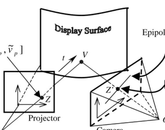
We model the projector display surface as a dense, regular, 3D mesh in the projector space. We typically use one 3D vertex (V) for each 2D pixel (Z) in the projector’s image plane, although a less dense mesh could be used if appropriate for the surface. As depicted in Figure 2, we position the camera so that it can see the entire display surface. During the normal ongoing operation of the system we continuously choose sample points in the known projector image and attempt to match them with the corresponding points in the camera’s image of the actual display surface. We do this for one sample point at each frame, refining the overall mesh continuously over time.
Figure 2. V is the point where the ray OpZ
terminates on the display surface. V is uniquely determined by a parametric value t. V’s projection (
Z
'
) on the camera image plane is constrained to lie on the epipolar line.Conceptually, each vertex
V
=
[
x,y,z
]
Tof the mesh lies on a ray extending from the center of projection of the projector (Op) through the corresponding 2Dpixel Z in the projector's image plane. For each 2D projector pixel Z we want to converge on, and then continuously maintain an accurate estimate for the scalar parameter t corresponding to the normalized distance along the ray where the ray terminates on the display surface at V. Figure 2 depicts the geometry of the setup.
From [Fauge93], we know that for a given 3 × 4 Z V t Z’
]
~
,
~
[
u
cv
c Epipolar Line Camera Oc Projector Op]
~
,
~
[
u
pv
pprojection matrix (Mp), and a sample point
T p p
v
u
Z
=
[
~
,
~
]
on the projector’s image plane, if we rewrite Mp asM
p=
[
p
~
p
]
, where p is a 3 × 3 matrix andp
~
is a 3×1 vector, V can be computed as)
1
~
~
~
(
1
+
−
=
− p pv
u
t
p
p
z
y
x
Equation 1where t is a parametric scalar value. Each sample point Z when projected onto the display surface has a corresponding projection Z’ in the camera's image space. Given the projection matrix Mcof the camera
we could estimate t using a traditional correspondence approach (a standard review is presented in [Dhond89]). Because the observations of the feature positions are noisy, and the various system parameters uncertain, we use a Kalman filter [Brown97, Maybe79, Welch97a] (a predictor-corrector based minimum-variance stochastic estimator) to estimate the parametric value t for every projector pixel Z and corresponding mesh vertex V. We use the prediction step of the Kalman filter to estimate where the Z should appear on the display surface, and subsequently to limit the feature search in the camera image to a relatively small region. When a match is found, the difference between the prediction and the actual match is used to correct the filter's estimate of the parameter t, and thus the 3D point V.
For each 2D projector pixel Z we use an independent Kalman filter to estimate the parametric value t that corresponds to the projection of Z on the display surface, as seen in the actual camera measurement. Together with the projector parameters each parameter t determines the 3D position of each mesh vertex V. We use a position-only (no velocity) dynamic model for each parameter, i.e. we assume that the parameter is a constant with only a small amount of zero-mean normally distributed white noise perturbing it over time.
Because the perspective projection is not linear, we employ an Extended Kalman filter (EKF) as described in [Brown97, Maybe79, Welch97a]. We use the following measurement model:
[
]
c c T c T c cs
v
s
u
z
y
x
M
h
v
u
,
=
(
,
,
,
)
=
[
′
,
′
]
where T c T c cv
s
M
x
y
z
u
,
,
]
[
1
]
[
′
′
=
Following conventional Kalman filter notation we denote the estimated 1D error covariance of t as Pk,
and the 2D measurement variance of
[
u ~
~
c,
v
c]
T as Rk.Assuming the measurement variance is equal and independent, we can write Rkas
=
k k kr
r
R
0
0
So the time update equations are filter are
Q
P
P
t
t
k k k k+
=
=
− + − + 1 1 Equation 3And our measurement update equations are
[
]
− − − − −−
=
−
+
=
+
=
k k k k T c c T c c k k k k T k k k k k kP
H
K
I
P
v
u
v
u
K
t
t
R
H
P
H
H
P
K
)
(
)
]
,
[
~
,
~
(
)
(
1Where Hkis the Jacobian matrix of the measurement
function with respect to t,
T k c k c k
t
v
h
t
u
h
H
∂
⋅⋅
⋅
∂
∂
⋅⋅
⋅
∂
=
(
)[
]
(
)[
]
.The time update (Equation 3) is used to predicate parametric value t and error covariance P at the current time. The measurement update (Equation 4) is used to correct the predictions based on the actual measurement. After each time-measurement update pair, the 3D position of V is updated corresponding to the new tkusing Equation 1.
We initialize our algorithm with a rough estimate of the display surface (some practical constraints), with every parameter t set to 0.5, corresponding to the middle point between the far and near plane. Then we refine the estimates iteratively over time, measuring a distinct point at each frame. For each iteration we do the following:
1. capture an image of the display surface, and make a copy the contents of the projector’s frame buffer;
2. choose a projector pixel V, select a small sample of neighboring pixels, and search for the sample in the neighborhood of the predicted location in the camera’s image; 3. perform the Kalman Filter update for the
corresponding projector pixel; and
4. use 2D Delaunay Triangulation [Delau34] to update the mesh.
We repeat this process continuously while the system is being used. Notice that in the time update (Equation 3) we add a small amount of process variance Q to compensate for slow changes in the system. Q should not be zero, or the Kalman filter will cease to update its estimate of the display surface after it has converged to a “solution.” With the added process variance the filter is never allowed to be
Equation 4
absolutely certain of the parameters, and so it continues to adjust the estimates very slowly, accounting for changes due to drift or other factors.
Selection of Feature Points
Because of computational constraints we cannot compute an entire feature set (all projector pixels) in one iteration. Instead we select and update sequentially a small number of feature points at each iteration, in a single-pixel-at-a-time fashion similar to [Welch97b]. The selection process has two parts: pseudo-random selection and distance-based selection. In the pseudo-random selection, we first define a list of sample points, and then permute the list. At each iteration, a number of consecutive points in the permuted list are selected in a way that each point has equal likelihood of being updated.
In the distance-based selection, we want to identify possible outlying points (large uncertainty and large residual) and correct them as soon as possible. We found that in practice, such points tend to be far away from the correct points in 3D. We use a selection process based on Euclidean distance. We define a maximum neighborhood distance (MND). For every sample point (Z) that has been updated, we find its closest neighbor (Zn) that also has been updated at
least once. If the distance between Z and Znis greater
than MND, this Z is considered a point with higher uncertainty, and added to the selected point list. One may argue that this distance-based selection imposes an assumption of the display surface geometry—no two neighbor points can be farther than MND—but in fact, this selection only tries to identify possible outlying points. If a point with high uncertainty turns out to be a correct one, it will converge to that position in subsequent updates. In practice, we set the MND to be twice the distance between two neighboring feature points with the initial estimate (t = 0.5). We found this MND works well for the variety of display surfaces we have experimented with.
Predicative Pattern Match
Once we have a selected sample point, we want to find its corresponding point in the camera image. Using the current parametric value t and the estimated error variance Pk, we compute the closest
point ( Zmin) and the furthest point ( Zmax), where Zmin
is computed as t-sqrt(Pk), and Zmax is computed as
t+sqrt(Pk), where sqrt is the square-root operation.
The two points Zmaxand Zminare projected back to the
camera image plane, forming a line on the image plane along the epipolar line. We create a bounding box around this line using the estimated error covariance Pk, and then perform the search within this
box. The estimated error variance Pkwill gradually
decrease as the Kalman filter converges. The bounding box will correspondingly shrink as Pk
decreases. Consequentially, the search area will become smaller and smaller until the system reaches a steady state.
For our setup, we use a 16x16 block around each selected sample point as the correlation template. We use the Matrox Imaging Library (MIL) to perform the pattern matching within the specified bounding box in the camera image. It returns a match with sub-pixel accuracy. In some cases, there are multiple matches returned by the MIL, all within the bounding box. In such case we compute the mean and the standard deviation of these matches, and if the standard deviation is greater than the measurement variance Rk,
the entire match set is discarded. Otherwise, we use the mean as the final result.
Because MIL's template matching routine searches within the entire bounding box, sometimes it will return a match that is not on the epipolar line. This is likely due to two factors: there is likely to be error in the a priori estimated internal and external projector and camera parameters, and there is some amount of noise (electronic) in the digitized images. If such a situation is encountered, we compute its distance to the epipolar line, and if the distance is greater than sqrt(rk) (the presumed measurement variance) the
match is discarded. Figure 3 depicts such a situation. Image rectification is widely used in stereo algorithms. It is a two-dimensional transformation that attempts to align the epipolar lines along (parallel to) image scan lines, so that the search for correspondence is computationally more tractable. We do not rectify our images because the number of points we compute at each iteration is typically small for our setup, and rectification would cost more than the speedup it brings in the search phase. Recall also that our primary goal is not speed, as the operations continue throughout normal operation, not as an off-line calibration. We use the MIL library’s template matching function. Its hierarchical search algorithm is very fast, and we have found no significant difference between a search along a line or within a box. Finally we check the result returned by the MIL routine to see if it is within our estimated measurement deviation of the epipolar line.
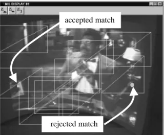
Figure 3. A screenshot of the system during
autocalibration of a curved display surface with video imagery. Here the system is updating 10 sample points per frame. For illustrative purposes we modified the code to render the bounding box (the search area) and epipolar line corresponding to each sample point. Two candidate matches are shown: the small square on the left indicates an accepted match, while the dot on the right indicates a rejected one because it is too far away from the epipolar line.
Rendering Correct Image
We use a two-pass technique as described in [Raskar98] to render perspectively correct images using our continually updated estimate of the display surface. To do this, we first need to create a triangular mesh. We implemented a scan-line based triangulation routine to create a complete mesh and let it deform as its vertices’ 3D positions were being updated. In practice we found that until the system reached a steady state, this approach created noticeable distortions if there was a “hole” in the mesh. (A “hole” exists where there are updated points surrounding points that have not yet been updated.) To address this we chose to perform a complete triangulation in run-time. Assuming there is no self-intersection of the display surface, the triangulation can be performed in projector’s screen space using a 2D Delaunay triangulation method, which is relatively simple to implement, and more robust than its 3D counterpart.
Because rendering is not our primary focus, we have not yet spent significant effort to achieve fast rendering speeds. We have a very basic OpenGL program that offers enough to demonstrate that the surface estimate was correct. (This can be seen in video.) We have identified several places the rendering could be optimized, and we also have an eye on continually improving graphics hardware.
Fundamentally the rendering and surface estimation are largely de-coupled in our method.
4. EXPERIMENTS RESULTS
We implemented our approach using C++ under Windows NT. We initially developed and tested our algorithm in simulator where we could perform controlled experiments. We then transformed the simulator into a working system. (The primary difference between the simulator and the real setup is that in the real setup we initially have to estimate the external and internal parameters of the camera and the projector.) We first present some results from our simulator, and then some results using our real setup. To make our results more realistic in our simulation, we used the external and internal parameters of the camera and the projector, estimated from the real devices. All of our experiments (simulated and actual) have the same basic setup: the projector is about one meter away from the display surface, and the camera is about 0.6 meters up and to the right of the projector, pointing at the display surface.
In our simulations we set the process noise covariance Q to (1e-5)2 and the initial error covariance Pkto (5e-1)2(both have units of parameter
t squared), and the measurement variance rk to 32
(pixels squared). We used a 40 x 30 mesh of feature points. We performed two experiments: one using a planar display surface with a sharp discontinuity, and another using a curved (concave) surface. To reinforce the independence of the approach from the graphical content, we used a short sequence of video from a commercial film. In practice the imagery would be the ongoing stream of whatever the user was displaying—2D windows or 3D graphics. We started the system with estimates that corresponded to the rough 3D bounding boxes of the surfaces, and let the system run about 45 minutes in each experiment. In simulation we were able to assess the absolute accuracy of our results, as shown in Table 2. The estimated surfaces are shown in Figure 4 and Figure 5 respectively. Mean Error (mm) Max. Error1 (mm) Planar Surface 2.41 6.78 Curved Surface 1.39 5.23 Table 2. Accuracy of the Simulation
1
The results shown here do not include candidate outlier points selected by distance-based selection routine. accepted match
Figure 4. Planar surface simulation. Blue
surface is the actual surface; red dots are the estimated feature points. Light blue dots (magnified for illustration purpose) are selected outlying points detected by our distance-based heuristic.
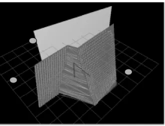
Figure 5. A bird-eye view of the curved surface
simulation.
Figure 6. The estimate of a curved display
surface after we run our algorithm for over one half hour in a real setup.
Figure 6 shows the results for a curved surface in a real setup. Panels (a) and (b) of Figure 1 show the difference between an uncorrected view and a corrected view. (Note that in our real setup we had no accurate ground truth to compare our results with.) Notice how the wall is curved and the window has a discontinuity in Figure 1 (a), and how they appear straight and continuous in Figure 1 (b). More results are shown in the video.
5. CONCLUSION
Beyond large display systems such as [Curz93, Li00] we are excited by the growing prospect of graphical imagery displayed on real surfaces around us [Raskar98, Under97, Under99]. We believe that our approach to surface estimation provides an important piece of the puzzle. The approach is accurate, robust, and can be implemented in practice with reasonably common components and minimal infrastructure. Furthermore, we have done some preliminary work on extending our method to include continual estimation of other system parameters, such as camera and projector poses, which can vary over time. The primary challenge is the limited observablity [Soatt94] because of the very constrained motion of projectors and cameras. We are planning to impose metric constraints on the state space to reduce the set of indistinguishable states.
Beyond the algorithmic improvements we present here, we look forward to improved hardware. For example, some day “smart projectors” with built-in cameras will be common, enabling automatic adjustments beyond simple keystone correction. Some day graphics engines will support more efficient rendering onto non-planar (and non-rectangular) surfaces, and maybe will even support automatic view-dependent correction.
ACKNOWLEDGEMENTS
This research is supported by the National Science Foundation agreement ASC-8920219: "Science and Technology Center for Computer Graphics and Scientific Visualization", Intel Corporation, and the "National Tele-Immersion Initiative" sponsored by Advanced Networks & Services, Inc. We would like to thank members of the Office of the Future group at UNC Chapel Hill, and in particular Prof. Henry Fuchs and Herman Towles for useful discussion and support.
REFERENCES
[Alon00] Jonathan Alon and Stan Sclaroff, Recursive Estimation of Motion and Planar Structure, Proceeding of IEEE Conference on Computer Vision and Pattern Recognition (CVPR 2000). [Azarb95] Azarbayejani, Ali, and Alex Pentland,
June 1995, Recursive Estimation of Motion, Structure, and Focal Length. IEEE Trans Pattern Analysis and Machine Intelligence, June 1995, 17(6).
[Broid91] T. Broida and R. Chellappa. Estimating the kinematics and structure of a rigid object from a sequence of images. PAMI, 13(6):497-513, 1991.
[Brown97] Brown, R. G. and P. Y. C. Hwang. 1997. Introduction to Random Signals and Applied Kalman Filtering, Second Edition, John Wiley & Sons, Inc, 3rd edition.
[Curz93] Curz-Neira, Carolina et al., 1993 Surround-Screen Projection-Based Virtual Reality: The Design and Implementation of the CAVE, SIGGRAPH Conference Proceedings, Annual Conference Series, Addison-Wesley, July 1993.
[Delau34] B. Delaunay. Sur la sph`ere vide. Izv. Akad. Nauk SSSR, Otdelenie Matematicheskii i Estestvennyka Nauk 7 (1934), 793--800 [Dhond89] U. Dhond and J. Aggrawal. Structure
from stereo: a review. IEEE Transactions on Systems, Man, and Cyber-netics,
19(6):1489–1510, 1989.
[Fauge93] O. Faugeras, Three-Dimensional Computer Vision: A Geometric
Viewpoint,Cambridge, Massachusetts; MIT Press, 1993.
[Fuchs99] H. Fuchs, M. Livingston, G. Bishop, and G. Welch, "Dynamic generation of imperceptible structured light for tracking and acquisition of three dimensional scene geometry and surface characteristics in interactive three dimensional computer graphics applications". US Patent, US 5870136, 1999, pp. 1-20.
[Humph99] Greg Humphreys and Pat Hanrahan, 1999, A Distributed Graphics System for Large Tiled Display, in the Proceeding of IEEE Visualization 1999.Oct. 1999. [Li00] Kai Li, et al. Early Experiences and
Challenges in Building and Using A Scalable Display Wall System. IEEE Computer Graphics and Applications, vol 20(4), pp 671-680, 2000.
[Matth88] L. Matthies, R. Szeliski, and T. Kanade, Kalman Filter-based Algorithms for Estimating Depth from Image Sequences, Tech. report CMU-RI-TR-88-01, Robotics Institute, Carnegie Mellon University, January 1988
[Maybe79] Maybeck, Peter S. 1979. Stochastic Models, Estima-tion, and Control, Volume 1,
Academic Press, Inc.
[Raskar98] Raskar, R. et al., 1998, The Office of the Future: A Unified Approach to Image-Based Modeling and Spatially Immersive Displays. SIGGRAPH Conference Proceedings, Annual Conference Series, Addison-Wesley, July 1998.
[Raskar99] R. Raskar, M, Cutts, G. Welch, and W. Stürzlinger, 1999, Efficient Image Generation for Multiprojector and Multisurface Display, in the Proceedings of the Ninth Eurographics Workshop on Rendering, (Vienna, Austria), June 1998
[Saman99] R. Samanta et al., “Load Balancing for Multi-Projector Rendering Systems,” Proc.1999 Eurographics/Siggraph Workshop on Graphics Hardware, ACM Press, New York, Addison-Wesley, Reading, MA, Aug. 1999, pp.107-116. (See also
http://www.cs.princeton.edu/omnimedia/inde x.html, cited 12 Oct. 2000.)
[Soatt94] Stefano Soatto. Observability/ identifiability of rigid motion under perspective projection, Proc. of the 33rd IEEE Conf. on Decision and Control, CDC 1994.
[Under97] J. Underkofler, “A View from the Luminous Room,” Personal Technologies, Vol.1, No.2, June 1997, pp. 49-59. [Under99] J. Underkofler,B. Ullmer,and H.Ishii,
“Emancipated Pixels:Real-World Graphics In The Luminous Room,”Computer Graphics, Annual.Conference.on Computer Graphics and Interactive Techniques, A.Rockwood, ed., Siggraph Conference Proc.,ACM Press, New York, Addison-Wesley, Reading, MA, 1999, pp.385-392.
[Welch97a] Greg Welch and Gary Bishop, 1997. An Introduction to Kalman Filter. Technical Report, TR 95-041, Dept. of Computer Science, University of North Carolina at Chapel Hill, Chapel Hill, NC
[Welch97b] G. Welch and G. Bishop, "SCAAT: Incremental Tracking with Incomplete Information," in Computer Graphics, Annual Conference on Computer Graphics & Interactive Techniques, T. Whitted, Ed., SIGGRAPH 97 Conference Proceedings ed. Los Angeles, CA, USA (August 3 - 8): ACM Press, Addison-Wesley, 1997, pp. 333-344.