APPENDICES
A. Economic Analysis
When seeding is required by regulatory revegetation obligations, determining the most cost effective option is relatively straight forward. Listing total costs associated with different methods, or suppliers, to accomplish the task is sufficient. However, when seeding is an optional consideration, the economic efficiency of the project requires a more critical evaluation. A selected project should be efficient—meaning that it yields positive net benefits.
The challenges of applying full cost-benefit analysis to projects on Crown land was explained in Chapter 2. For projects on private land, and for some situations on Crown land, where project impacts can be clearly linked to a specific enterprise like a ranch or a community pasture, cost–benefit analysis should be applied. Despite uncertainties around future revenues and other assumptions, cost– benefit analysis can help to clarify management alternatives, and lead to more financially sound decision making.
The purpose of this appendix is to provide a simple example of cost–benefit analysis for a pasture seeding project. The principles demonstrated here can be used to evaluate other types of projects in a variety of situations. This type of analysis, however, does not evaluate the overall profitability of a livestock enterprise or ranch. The example is hypothetical, and different results can be expected if different estimates and assumptions are used.
Net Present Value
For the purposes of this example, the cost–benefit analysis is based on the net present value (NPV) of the seeding project or project alternative. The NPV is the difference between the present value of the estimated benefits (revenues) and the present value of the costs:
NPV = PV(Benefits) - PV(Costs)
If only one project option is being considered and the NPV for the project is positive, then it is considered efficient and can go ahead. If more than one project alternative is being evaluated, then the project with the highest NPV should be selected.
Information required
In the pasture context, seeding projects are usually planned to increase and maintain forage production over a period of years. Costs associated with seeding are an investment to receive an annual return in the form of additional forage production, which increases revenues. There may also be annual costs created by the project that must be deducted from additional annual revenue. This aspect of the analysis is sometimes referred to as partial budgeting, since it considers only those parts of the enterprise’s budget affected by the project. There is a general assumption with the analysis that the proposed project does not require a complete restructuring of the enterprise, and fits with the current management structure.
Costs
Costs can be variable and specific to the enterprise and location. For example, costs for land preparation can be lower than reported custom rates if older equipment is used.
Direct fixed costs would include: • site preparation,
• seed,
• seed application,
• additional fencing or livestock water development. Indirect fixed costs would include:
• risk associated with a failed seeding, • non-use during establishment, • future renovation requirements,
• interest on direct costs during the non-use period. Annual use costs might include:
• fence maintenance or fence moving in the case of portable electric fence that is specific to the seeding alternative,
• water maintenance associated with the project.
Benefits
The expected benefits (revenues) from increased forage production can be challenging to estimate, and are dependent on site conditions, species and seasonal precipitation. NPV is especially sensitive to the forage production estimates used in the analysis. Research and local knowledge should be consulted to develop production estimates. The valuation method for the added forage production can vary as well. One approach is to consider how the forage might be valued in the local pasture rental or lease market in $/AUM. If the extra forage can be used to extend the grazing season for the livestock enterprise, it may have higher value than the general pasture lease rate.
Increased forage production can also be equated to additional livestock
production; however, this approach is more complex and expands the amount of partial budgeting required for the cost-benefit analysis. The example presented here will use the pasture lease rate as the method for valuing the additional forage created by the seeding project.
Total herbage dry matter production in kg/ha or lbs/acre can be converted to AUMs by using an appropriate utilization factor (e.g., 50–70%), and a value for the forage consumption required by one animal unit for one month. This figure can vary depending on the size of the typical animal unit. Traditionally this value has been about 364 kg (802 lbs) based on a daily consumption of 12 kgs (26 lbs) for a 454 kg (1,000 lb) cow with her suckling calf. Larger frame crossbred cows can weigh as much as 545–636 kg (1,200–1,400 lbs), and these animals can consume as much as 14–27% more forage than the smaller 454 kg (1000 lbs) cow.
These differences should be kept in mind when determining the value of additional forage, especially when pasture lease rates and/or other estimates or conversion factors are used. The goal is to match the grazing with an appropriate pasture lease rate and the actual increase in forage created by the seeding. In the example presented here, production estimates in AUMs per acre were derived from a combination of reported stocking rates and herbage production. Browse production should also be considered if it is expected to be an important source of forage during the grazing season.
While all the investment costs of a seeding project are incurred in present values, revenues are realized annually over a period of years. These benefits received in the future are worth less than the same amounts received today, and therefore must be discounted to present value so they can be compared directly to costs (see net present value above).
Choice of discount rate can have a significant effect on the determination of the present value of benefits. The pasture lease rates used in this example are projected into the future and are not adjusted for inflation. Therefore, it is appropriate to use a “real” rather than nominal or inflation adjusted discount rate, or loan rate. Bank loan interest rates are typically composed of a real rate of return, and an expected inflation rate. In the example presented here, a base or real discount rate of 4% is assumed. An additional 4% discount is added to reflect a real rate of risk associated with the project. It is also acceptable to account for risk associated with seeding establishment, by adding the cost of re-seeding and additional project delay to the investment cost as noted above. However, in the example developed here, risk associated with the forage production projected over the longer term is perhaps more significant than establishment failure. The 4% added to 4% discount rate accounts for both types of risk, and provides a reasonably conservative analysis.
Example Pasture Development Options
The project options used in this example are based in the Northeast–Peace-Liard region approximately 30 km west of Dawson Creek. Recent aspen logging on 120 acres has created an opportunity to consider improving forage production with seeding. The life of each option is expected to be 15 years. The options are:
A) Piling of remaining logging slash and remaining stumps, followed by double discing (with heavy breaking disc), fixed-wing aerial broadcast seeding of agronomic species and floating. The land is already perimeter fenced. A single water trough will be installed and gravity
fed from an existing dugout. After the year of establishment, the pasture will be continuously grazed for a four month period on annual basis. This scenario is considered a conventional clearing and breaking treatment, and expected to minimize aspen regrowth for the life of the project. The expected production, expressed as a stocking rate, is 2.4 AUMs/acre.
B) There is no seeding after logging. Forage production is provided by the native plant community, and aspen regrowth is controlled with intensively managed grazing. To facilitate intensive stocking, a single high tensile smooth wire electric cross fence is installed. This wire is used to electrify a portable poly-wire electric fence which is moved to allow strip grazing. Water is provided by six gravity-fed troughs. The expected production is 0.6 AUMs/acre including use of aspen browse. C) Logging slash and stumps are piled and burned, and the area is
aerially seeded with a fixed-wing aircraft. Livestock are turned out for a brief period after seeding to provide some disturbance and increase seed-to-soil contact. Water development and electric fence are installed as in scenario B above, to manage grazing and potential aspen regrowth. Expected production is 3 AUMs/acre.
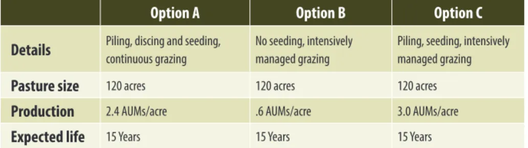
Pasture development option details and assumptions are summarized in Table A.1. Costs and benefits for each option are summarized in Table A.2.
Table A.1 Summary of pasture seeding options for cost–benefit analysis example.
Option A Option B Option C
Details Piling, discing and seeding, continuous grazing No seeding, intensively managed grazing Piling, seeding, intensively managed grazing
Pasture size 120 acres 120 acres 120 acres
Production 2.4 AUMs/acre .6 AUMs/acre 3.0 AUMs/acre
Table A.2 Costs and benefits associated with pasture seeding options.
Costs Rate Option A Option B Option C
Piling (D7 or equivalent) 1.0 acre/hr x $175/hr x 120 ac. 21,000 0 21,000
Double disc $25/acre x 2 x 120 ac. 6,000 0 0
Seed $2.20/lb x 15 lbs/ac x 120 ac. 3,960 0 3,960
Aerial seeding $7.50/acre x 120 ac. 900 0 900
Floating/rolling $15.00/acre x 120 ac. 1,800 0 0
Electric fencing costs 0 2,500 2,500
Water - 1" poly pipe 250 1,000 1,000
Water tanks 300 1,500 1,500
Tank floats 50 300 300
One season lost use 72 AUMs @ $15 each 1,080 0 1,080
Interest during non-use 8% of direct costs 2,736 0 2,469
Total Investment $38,076 $5,300 $34,709
Additional annual costs ($)
Labour 40 hrs @ $15/hr 0 600 600
Additional annual revenues
Total AUMs AUMs/acre x 120 ac. 288 72 360
Revenue @ $15/AUM Total AUMs x $15/AUM $4,320 $1,080 $5,400
Net revenue @ $15/AUM Annual revenue – annual cost $4,320 $480 $4,800 Revenue @ $20/AUM Total AUMs x $20/AUM $5,760 $1,440 $7,200 Net revenue @ $20/AUM Annual revenue – annual cost $5,760 $840 $6,600 Annual labor costs are incurred for options B and C to support increased
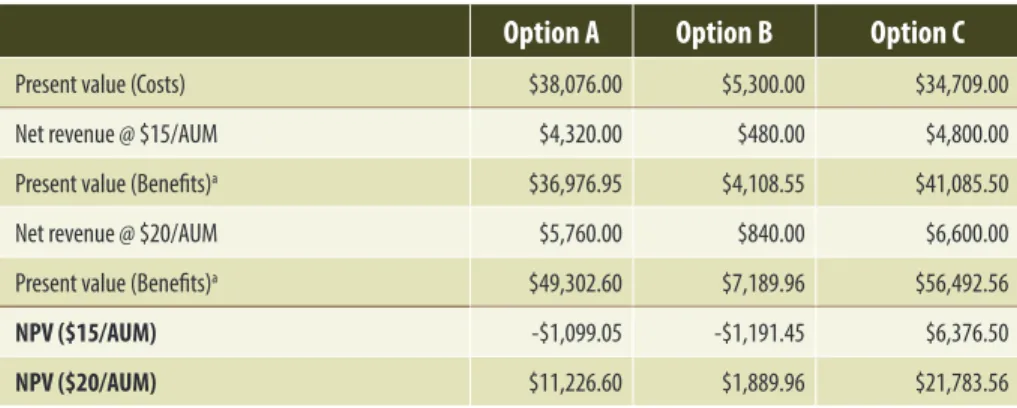
water development maintenance and movement of portable electric fence for intensively managed grazing. This decreases net revenues for those options. Net annual revenues are converted to present value for the 15 year period using a discount rate of 8% which includes a real discount rate of 4% and a risk allowance of 4%. Net present values can be calculated using the NPV financial function in Microsoft Excel. The present value of benefits and the NPV for each pasture development option is presented in Table A.3.
Table A.3 Summary of present value costs, annual net revenues, present value of benefits over 15 years, and NPV for pasture development options.
Option A Option B Option C
Present value (Costs) $38,076.00 $5,300.00 $34,709.00
Net revenue @ $15/AUM $4,320.00 $480.00 $4,800.00
Present value (Benefits)a $36,976.95 $4,108.55 $41,085.50
Net revenue @ $20/AUM $5,760.00 $840.00 $6,600.00
Present value (Benefits)a $49,302.60 $7,189.96 $56,492.56
NPV ($15/AUM) -$1,099.05 -$1,191.45 $6,376.50
NPV ($20/AUM) $11,226.60 $1,889.96 $21,783.56
When forage production is valued at $15/AUM, only option C, which involves partial development, seeding and intensively managed grazing, results in a positive NPV. This suggests option C should proceed over all others under the assumptions used in the analysis. Both options A and B have negative NPV values suggesting neither should be implemented. When forage is valued at $20/AUM all options have positive NPV, but again option C should be pursued over the other options as it has the highest overall NPV.
Option B provides an interesting point for discussion, as it might be considered the lowest cost option of the three. However, forage production remains low under this alternative and thus the present value of benefits (revenues) is also low. Additional annual labor costs for the intensively managed grazing under this alternative also have a negative effect on NPV. If this option were changed to continuous grazing, eliminating electric fencing, additional water troughs, and the annual labor, the expected life would be shortened to seven years because of expected aspen regrowth. With these adjustments, option B would almost rival option C when a forage value of $15/AUM is used (NPV = $5,023, not in table). However, at the higher forage value rate of $20/AUM, option C far surpasses the modified option B. To make modified option B fully comparable, the future cost of a rejuvenation treatment to control aspen regrowth at year seven should be incorporated to extend the life of the alternative to 15 years (see footnote). The important message here is that increased forage production is the key to increased revenues, and if increased production can be achieved at a lower cost, net benefits (revenues) will be maximized. The main value of the cost-benefit analysis is that it allows full exploration of alternatives. Once the cost and revenue structure is set up in an Excel spreadsheet, any number of alternatives can be explored, and the most economically efficient alternative selected.
2 Options should be evaluated over the same discounting period so they have the same opportunity to
accumulate costs and benefits. Alternatives with different time periods can be compared by converting the NPVs to an equivalent annual net benefit. This is accomplished by dividing the NPV of each alternative by an annuity factor that has the same term and discount rate as the project itself (i.e., the present value of an annuity of $1 per year for the life of the project discounted at the rate used to calculate the NPV). In the example above, modified option B (with continuous grazing, a seven year life, an 8% discount rate and $15/ AUM forage value) has a NPV of $5,023. Its annuity factor (taken from a standard annuity table) is 5.206. Therefore the equivalent annual net benefit is $965 ($5,023 ÷ 5.206). The equivalent annual net benefit for alternative C ($15/AUM and 8% discount rate) is $745 ($6,376 ÷ 8.559). This assumes that modified option B could be rejuvenated at very low cost at the end of year seven, and this is an unrealistic assumption. To properly compare modified option B to other alternatives, the future cost of a rejuvenation to extend the pasture life to 15 years should be incorporated into the analysis.
References:
Alberta Agriculture and Food, 2007. Using the Animal Unit Month (AUM) Effectively, Available at: http://www1.agric.gov.ab.ca/$department/
deptdocs.nsf/all/agdex1201/$file/420_16-1.pdf [Accessed March 25, 2012]. Boardman, A. et al., 2011. Cost-benefit analysis: concepts and practice 4th ed.,
Upper Saddle River, N.J.: Prentice Hall.
Bork, E.W., Gabruck, D. & Klein, B., 2008. Trembling Aspen: Comparitive strategies to manage aspen in Canada’s Parkland Greencover Canada Program. Government of Alberta, Agriculture and Rural Development, 2011. Custom Rates
Survey Summary 2011. Available at: http://www1.agric.gov.
ab.ca/$department/deptdocs.nsf/all/inf13379 [Accessed March 24, 2012]. Krzic, M. et al., 2005. Aspen regeneration, forage production, and soil compaction on harvested and grazed boreal aspen stands. BC Journal of Ecosystems and Management, 5(2), pp.30–38.
LaRade, S., 2010. Long-term agronomic and environmental impact of aspen control strategies in the Aspen Parkland. University of Alberta. Available at: http://hdl.handle.net/10402/era.27433.
Robinson, J. & Burton, S., 2002. Increased Forage by Intensively Managed Controlled Grazing of Logged Lands, Peace River Forage Association of BC. Available at: http://www.peaceforage.bc.ca/ forage_facts_pdfs/FF_12_intensive_grazing.pdf.
Ruyle, G. and Ogden, P., 1993. What is an AUM? In R. Tronstad and George Ruyle, eds. Arizona Ranchers’ Management Guide. Arizona Cooperative Extension. Available at: http://ag.arizona.edu/arec/pubs/rmg/1%20 rangelandmanagement/01%20Rangeland%20ManagementSect.pdf [Accessed March 25, 2012].
Vallentine, J., 1980. Range development and improvement,s 2d ed., Provo, Utah: Brigham Young University Press.
Wikeem, B. et al., 1993. An overview of the forage resource and beef production on Crown land in British Columbia. Canadian Journal of Animal Science, 73(4), pp.779–794.
Workman, J.P. & Tanaka, J.A., 1991. Economic feasibility and management considerations in range revegetation. Journal of Range Management, pp.566–573.
B. Soil Erosion Assessment Key – Climatic Precipitation Factors
Table B.1 Cariboo forest region: Precipitation factorsLow Moderate High Very high
all BG PPxh IDFxm IDFxw IDFdk IDFmw MSxk MSxc SBSdw SBSmc* SBSmh SBSmc* SBSmw SBSwk SBPSxc SBPSdc SBPSmc SBPSmk ESSFxv ESSFwk* ESSFwc ESSFwk ICHdk ICHmk ICHwk* ICHwk*
*These subzones/variants encompass two precipitation factor ranges. Use local experience in deciding the appropriate precipitationfactor to apply in the keys.
Table B.2 Kamloops forest region: Precipitation factors
Low Moderate High Very high
all BG PPxh IDFxh IDFxw IDFdk IDFdm IDFmw IDFww MSxk MSdc MSdm MSmm SBSdh SBSdw SBSmm SBPSmk ESSFxc ESSFdc ESSFdv ESSFwc ESSFmw ESSFvc ESSFvv ICHmk ICHmw ICHwk ICHvk CWHds CWHms
Table B.3 Nelson forest region: Precipitation factors
Low Moderate High Very high
PPdh1 PPdh2 IDFdm1 IDFdm2 IDFun IDFxh1 MSdk MSdm1 ESSFdc1 ESSFdk ESSFwc1 ESSFwc2 ESSFwc4 ESSFwm ESSFvc ICHdw ICHmk1 ICHmw1 ICHmw2 ICHmw3 ICHxw ICHwk1 ICHvk1
Table B.4 Prince George forest region: Precipitation factors
Low Moderate High Very high
SBSdh SBSdk SBSdw SBSmk1 SBSmc* SBSmh SBSwk SBSmw SBSmk2 SBSmc* SBSvk BWBSdk BWBSmw2 BWBSwc3 BWBSmw1 BWBSwc1&2 ESSFmm ESSFmv ESSFwk* ESSFwc ESSFwk* ESSFvc All SWB ICHmc ICHmm ICHwk* ICHvk ICHwk*
* These subzones/variants encompass two precipitation factor ranges. Use local experience in deciding the appropriate precipitation factor to apply in the keys
C. Seeding Rate Calculations
3Seeding recommendations often provide weight-based application rates, especially designed for growing agronomic or native species in field situations. They are frequently provided for broadcast methods as well, often with advice to double the rate normally suggested for drilled or direct seeding to compensate for sub-optimal seedbed conditions. Weight-based recommendations are fairly straight forward when species are seeded as a monoculture in a field, but are more complex for seed mixtures and when site conditions are less than ideal.
Seeding rates for agronomic species in ideal seedbed conditions are based on years of research and field trials. In situations that demand broadcast methods, site and seedbed conditions are highly variable and seeding rates are somewhat subjective. The number of suitable microsites for seed germination should also be a factor when developing broadcast seeding rates.
Appropriate seeding rates for a wide variety of seeding methods, seed mixtures and conditions can be developed independently using:
• a target plant density,
• the number of seeds per unit weight for the species, • pure live seed (PLS) for the species in the seed lot, • a percent establishment factor.
Determining seeding rate using target plant density
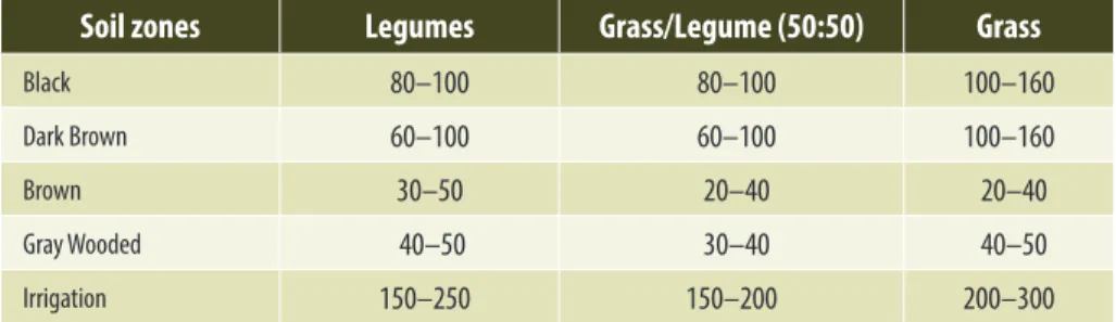
The target plant density is the number of plants of each species desired at the establishment stage when the plants are no longer reliant on food reserves in the seed and have sufficient root development to survive on the site. This is usually the number of plants established after the first growing season following seeding. In native plant communities, the target plant density will allow for the fact that many seedlings do not reach maturity, and that plant densities will be much lower at maturity (20–40% of established seedlings). For example, the target plant density for a native bunchgrass community may be 10 to 20 plants if a mature plant density of 4 plants/m2 is desired. Adjustments to this approach are required
for species that spread quickly by rhizomes or other means. Target plant densities for seeding native species can be estimated using reference plant communities. Table C.1 provides target plant densities for forage (pasture) seeding in the prairie soil–climatic zones as a reference. The Gray Wooded zone has application to the Northeast–Peace-Liard region, and parts of the north central interior (Bulkley-Nechako and Cariboo-Fraser Fort George). The seedling density for the brown zone may have some application for drier southern interior locations, but local experience and knowledge should be consulted.
3 Seeding rate calculation using target plant density adapted from A. Smreciu et al., Establishing Native
Plant Communities (Edmonton, AB: Alberta Agriculture, Food and Rural Development, 2002). Seeding rate formula attributed to D. Walker.
Table C.1 Suggested seedling density for forage seeding (plants/m2)
Soil zones Legumes Grass/Legume (50:50) Grass
Black 80–100 80–100 100–160
Dark Brown 60–100 60–100 100–160
Brown 30–50 20–40 20–40
Gray Wooded 40–50 30–40 40–50
Irrigation 150–250 150–200 200–300
Source: “Perennial Forage Establishment in Alberta” (Alberta Agriculture and Rural Development, 2005), http://www1.agric.gov.ab.ca/$department/deptdocs.nsf/all/agdex9682/$file/120_22-3.pdf?OpenElement.
The number of seeds per unit weight for a species in a seed lot can be taken from book values (see species summaries – Chapter 8), it can be obtained from a seed analysis lab or it can be determined from weighing actual seed counts. There can be wide variation depending on the variety or ecotype, and this can influence actual seeding rates. The actual value for the seed being applied should be used whenever possible. The pure live seed for the species in the seed lot can be obtained from the seed analysis certificate (Figure 7.2).
The estimate of establishment after the first growing season is used to develop an establishment factor in percent. This factor recognizes that under field conditions only a certain number of seeds and seedlings will make it through the germination and establishment stages and survive the first growing season (see Figure 6.1). Potential establishment also depends on individual species response to competition from seedlings of the same species, and seedlings of other species included in the mix. This can be an important factor for native species. Early successional species can be tolerant of high plant densities, while mid- to late-successional species may not grow as well in high density situations.
Table C.2 Typical estimates of seedling establishment (% seedlings per pure live seed after one season)
Establish-ment 25–50% 15–25% 5–15% 0.1–5.0% Species or type crested wheatgrass smooth bromegrass timothy perennial ryegrass cereal grains western wheatgrass northern wheatgrass slender wheatgrass Canada wildrye green needlegrass alpine fescues red fescue cultivars sheep/hard fescues alfalfa clovers tufted hairgrass junegrass Canada bluegrass many harvested native seeds
Seeding rate formula
Seeding rates for each species in a mix can be calculated with the formula below (see Example 1). If using target plant densities from Table C.1, the total suggested density should be apportioned to each species in the mix.
Target Plant
Density No. seeds per gram Pure live seed % Establishment % Conversion g/m
2 to Kg/ha plants m2 1 gram no. of seeds 1 PLS % 1 Estab. % 1 kg 1000 g 10,000 m2 1 ha x x x x x
Example 1: Seeding rate calculation for Rocky Mountain fescue using target plant density
Target plant density chosen for species = 20 plants/m2
Seeds per gram = 1,042 (from species summary pg. 112) PLS % = 88 Establishment % = 10 20 plants m2 1 1,042 1 0.88 1 0.10 1 kg 1,000 g 10,000 m2 1 ha
Each species in the mix can be calculated in this way. Increases in calculated rates may be required for broadcast applications, particularly when post seeding disturbance such as rolling, harrowing, or packing is not planned or is impractical.
Determining seeding rate using seed density
The seeding rate calculation and development of a seeding mix can be simplified by using recommended seeding densities in PLS/m2. These recommendations are
widely available for agronomic species seeded as monocultures, and are intended to achieve target plant densities that result in productive stands. These densities can be converted to kg/ha using the number of seeds per gram for the species and the same conversion factors used in the seeding rate formula above (see Example 2). For example, the recommended seeding density for wheatgrasses is 130–260 PLS/m2. Smaller seeded species generally have higher seed density rates,
to compensate for establishment factors (i.e., less food reserves than larger seeds; the recommended seeding rate for orchardgrass is 700-900 PLS/m2, and white
clover 750 PLS/m2).4 When combined in a seed mixture, recommendations can
typically range from 300 – 1,500 PLS/m2 depending on the species in the mixture,
seeding method and context.
Example 2: Seeding rate calculation for slender wheatgrass as a single species using recommended seed density in PLS/m2
Recommended density = 130–260 PLS/m2 (200 PLS/m2 chosen for this example)
Seeds per gram = 320 (from species summary page 112) PLS = 88% 200 PLS m2 1 320 1 0.88 1 kg 1,000 g 10,000 m2 1 ha
A seeding rate calculator, drill seeding rates for various row spacing, and additional seeding rate information for commonly used agronomic species is available at on line: http://www.agric.gov.ab.ca/app19/calc/forageseed/ forageseedintro.jsp
4 “Perennial Forage Establishment in Alberta” (Alberta Agriculture and Rural Development, 2005), http://
www1.agric.gov.ab.ca/$department/deptdocs.nsf/all/agdex9682.
x x x x x
x x x x =7.1 kg/ha