Multichannel Audio Modeling and Coding Using a Multiscale Source/Filter Model

(1)

University of Crete FO.R.T.H.

Department of Computer Science Institute of Computer Science

Multichannel Audio Modeling and Coding

Using a Multiscale Source/Filter Model

(MSc. Thesis)

Kyriaki Karadimou

Heraklion

November 2005

(2)

(3)

Department of Computer Science University of Crete

Multichannel Audio Modeling and Coding Using a

Multiscale Source/Filter Model

Submitted to the

Department of Computer Science

in partial fulfillment of the requirements for the degree of Master of Science

November 14, 2005 c

Author:

Kyriaki Karadimou

Department of Computer Science Board of enquiry: Supervisor Panagiotis Tsakalides Associate Professor Member Yannis Stylianou Associate Professor Member Apostolos Traganitis Professor Accepted by: Chairman of the

Graduate Studies Committee Dimitris Plexousakis Associate Professor Heraklion, November 2005

(4)

(5)

(6)

(7)

vii

Abstract

During the last decade, stereophonic audio is progressively being commercially substi-tuted by multichannel audio. The increase of the audio channels, both at the capturing and rendering sides, led to the creation of more realistic audio recordings that immerse the listener into the acoustic scene, but increased the requirements for transmission data rates as well. For this reason, many compression techniques have been proposed in order to give efficient solutions in several storage and transmission constraints. Consequently, multichannel audio compression algorithms have been developed which not only reduce the intra-channel redundancies, but the inter-channel redundancies as well. These algorithms, while very effective, remain highly demanding for many practical applications.

Therefore, this thesis proposes a source/filter model which divides the multichannel audio signal into two parts, a low-dimensional part that contains the microphone-specific information, and a high-dimensional part, which contains most of the inter-channel redun-dancy. By taking advantage of this redundancy among the channels we achieve very low data rate requirements, such as 10 kbps per channel for high quality coding (similar to the original recording). For comparison, current compression algorithms for multichannel audio such as Dolby AC-3 and MPEG-2 AAC have minimal bit rate requirements in the order of 64 kbits/sec/channel, for achieving acoustically indistinguishable encoding.

Another relevant issue is the fact that in order to create the multiple channels for multichannel audio rendering, a large number of microphones in a venue is used. These microphone signals are then mixed into a smaller number of channels that constitute the final multichannel audio recording. For various applications, methods that allow for remote mixing are of great interest in the music industry. Within our goals was to design an algorithm that can be used towards addressing such issues. Another area within our interests is remote collaboration of geographically distributed musicians, a field of great significance with extensions to music education and research. This innovative approach relaxes the current bandwidth constraints of these demanding applications, enabling their widespread usage and more clearly revealing their value.

The coding section of our model is based on a speech coding scheme, which estimates the probability density function of the source, giving a more compact representation of the transmission data and efficiently quantizes the estimated parameters with varying bit rate systems. This thesis, applies this coding method for the first time in the multichannel audio domain.

(8)

(9)

ix

PerÐlhyh

Ta teleutaÐa qrìnia sunteleÐtai mia meglh epanstash sto q¸ro thc anaparagwg c qou. Met th metbash apì ta analogik sust mata ston yhfiakì qo, ta stereofwnik sust mata anaparagwg c èqoun arqÐsei na dÐnoun th jèsh touc sta polukanalik, auxno-ntac ton arijmì kanali¸n anaparagwg c (hqeÐwn). Autì od ghse se pio realistikèc hqo-graf seic, oi opoÐec perikleÐoun (immerse) _{ton akroat me thn akoustik skhn , dÐnontac}

thn aÐsjhsh ìti brÐsketai sto q¸ro thc hqogrfhshc (p.q. sunauliakìc q¸roc). Apì thn llh pleur ìmwc, aut h posìthta plhroforÐac aÔxhse kai tic angkec apoj keushc kai apodotik c metdoshc eÐte mèsw DiadiktÔou, eÐte mèsw asÔrmatwn diktÔwn. Gia autì to lìgo èqoun anaptuqjeÐ prìsfata algìrijmoi gia th sumpÐesh polukanalikoÔ qou, pou mei¸noun ìqi mìno thn plhroforÐa kje kanalioÔ xeqwrist (intra-channel) all kai thn koin plhroforÐa pou pijanìn uprqei metaxÔ perissìterwn tou enìc kanali¸n (inter-channel). AutoÐ oi algìrijmoi, parìlo pou eÐnai exairetik apotelesmatikoÐ, exakoloujoÔn na jewroÔntai mh praktikoÐ gia pollèc efarmogèc ìpou to eÔroc metdoshc eÐnai idiaÐtera qamhlì.

Se autì to shmeÐo ja prèpei na anafèroume ìti mia polukanalik eggraf pragmatopoi-eÐtai me perissìtera mikrìfwna apì ton telikì arijmì twn kanali¸n thc hqogrfhshc. Ta mikrofwnik aut s mata qrhsimopoioÔntai gia th sÔnjesh thc polukanalik c eggraf c, mia diadikasÐa pou sun jwc anafèretai wc {mÐxh}(mixing) kai gÐnetai apì eidikoÔc me krit ria kurÐwc aisjhtik c kai empeirikèc gn¸seic. S mera, gia na metadojeÐ mia polukanalik hqo-grfhsh (p.q. mÐa zwntan sunaulÐa) mèsw yhfiakoÔ radiof¸nou, h parousÐa tou eidikoÔ gia th {mÐxh} sto sugkekrimèno q¸ro pou gÐnetai h sunaulÐa eÐnai aparaÐthth. EpÐshc, ìlh h diadikasÐa prèpei na gÐnei sto q¸ro autì. Sthn prxh, dhlad , aut h diadikasÐa apoteleÐ èna prìblhma kai eÐnai ènac apì touc lìgouc pou empodÐzoun s mera th metdosh zwntan¸n programmtwn polukanalikoÔ qou. Me th mèjodo pou parousizoume ja eÐnai dunat h ex apostsewc {mÐxh} polukanalikoÔ qou (remote mixing), h opoÐa èqei pollèc efarmogèc sth mousik biomhqanÐa. Mia llh efarmog ìpou den eparkoÔn oi uprqousec teqnikèc kwdikopoÐhshc eÐnai h ex apostsewc tautìqronh sunergasÐa mousik¸n. Aut jewreÐtai mia apì tic shmantikìterec efarmogèc eikonik¸n periballìntwn kai èqei apodei-qjeÐ ìti apaitoÔntai meglec taqÔthtec metdoshc gia thn sunergasÐa twn mousik¸n qwrÐc na gÐnontai antilhptèc oi qronikèc kajuster seic sth metdosh. 'Enac apì touc stìqouc loipìn, aut c thc metaptuqiak c ergasÐac eÐnai h parousÐash miac nèac mejìdou, h opoÐa ja periorÐzei touc lìgouc pou kajistoÔn tètoiec efarmogèc apotreptikèc sthn prxh (qamhlèc taqÔthtec metdoshc, duskolÐec sth {mÐxh}) kai epitrèpei thn eurÔterh qr sh kai explws touc.

H paroÔsa ergasÐa proteÐnei mÐa nèa mèjodo pou kwdikopoieÐ thn polukanalik mousik me polÔ qamhlèc taqÔthtec metdoshc. ProteÐnetai, sugkekrimèna, èna montèlo phg c/

(10)

fÐltrou, to opoÐo diaqwrÐzei thn koin plhroforÐa se ìla ta hqhtik kanlia apì thn plhroforÐa pou qarakthrÐzei to kje sugkekrimèno kanli. Me autì ton trìpo, h koin plhroforÐa mporeÐ na metadojeÐ mèsw tou diktÔou mìno gia èna kanli (kanli anaforc). Ta upìloipa kanlia ja anasuntejoÔn sto dèkth apì to kanli anaforc me th qr sh thc epiplèon plhroforÐac (h opoÐa ja prèpei na èqei ìso to dunatì mikrìterec apait seic se taqÔthta diktÔou). Ekmetalleuìmenoi loipìn, thn pleonzousa plhroforÐa tou kje ka-nalioÔ, epitugqnoume taqÔthtec metdoshc thc txhc twn 10 kbps _{gia kje kanli gia}

uyhl poiìthta kwdikopoÐhsh (parìmoia me thn poiìthta thc arqik c hqogrfhshc). En-deiktik anafèroume ìti sqetik sust mata sumpÐeshc polukanalikoÔ qou, ìpwc eÐnai ta dhmofil Dolby AC-3kaiMPEG-2 AAC,èqoun elqisth apaitoÔmenh taqÔthta metdoshc tou polukanalikoÔ qou 64 kbps/ kanli.

Tèloc, gia thn kwdikopoÐhsh twn paramètrwn tou proteinìmenou montèlou basizìmaste se èna sÔsthma kwdikopoÐhshc shmtwn fwn c, to opoÐo proseggÐzei th sunrthsh puknì-thtac pijanìpuknì-thtac thc phg c (parèqontac mÐa sumpuknwmènh anaparstash twn dedomènwn proc metdosh) kai kbantÐzei me apotelesmatikì trìpo tic paramètrouc tou montèlou me poikÐlouc rujmoÔc metdoshc. Na shmei¸soume se autì to shmeÐo ìti aut h mèjodoc kwdikopoÐhshc efarmìzetai sthn paroÔsa ergasÐa gia pr¸th for se polukanalikì qo. O endiaferìmenoc anagn¸sthc mporeÐ na brei perissìterec plhroforÐec sqetikèc me thn proteinìmenh mèjodo (sta ellhnik) sto Appendix B.

(11)

xi

EuqaristÐec

Se aut thn enìthta, xefeÔgontac proc stigm n apì to episthmonikì plaÐsio thc meta-ptuqiak c ergasÐac, ni¸jw thn angkh na euqarist sw ton patèra mou Dhm trio Karad mo, o opoÐoc pÐsteue se mèna, upost rize kje mou prospjeia kai ston opoÐo ofeÐlw se èna meglo bajmì autì pou eÐmai s mera. Akìmh, ja jela na euqarist sw th mhtèra mou Kalliìph Karad mou gia thn aperiìristh upost rix thc stic dÔskolec stigmèc mou ed¸ sto nhsÐ -qwrÐc aut tÐpote apì ìla aut de ja eÐqe sumbeÐ- kaj¸c kai tic poluagaphmènec mou adelfèc, Tatina kai MarÐa Karad mou.

Ja jela akìmh na euqarist sw ton epìpth mou k. Panagi¸th TsakalÐdh gia thn en-jrrunsh kai thn kajod ghs tou. Parìlo to fìrto twn upoqre¸se¸n tou wc prìedroc tan pnta par¸n me ousiastikèc sumboulèc basismènec tìso stic episthmonikèc tou gn¸-seic ìso kai sthn poluet empeirÐa tou ston ereunhtikì tomèa. Ton euqarist¸ kai elpÐzw na stjhka xia twn prosdoki¸n kai thc empistosÔnhc tou. EÐmai akìmh idiaÐtera eugn¸-mwn sto deÔtero epìpth mou kai eidikì ston tomèa tou polukanalikoÔ qou k. Ajansio Mouqtrh, qwrÐc thn ousiastik sumbol tou opoÐou de ja eÐqe oloklhrwjeÐ h paroÔsa ergasÐa. Ton teleutaÐo enmish qrìno eÐqame mÐa yogh kai euqristh sunergasÐa kat th dirkeia thc opoÐac kèrdisa pra poll.

Sth sunèqeia ja jela na euqarist sw gia th summetoq touc kai tic qr simec parath-r seic touc kai ta lla dÔo mèlh thc epitrop c exètashc thc metaptuqiak c mou ergasÐac ton k. Apìstolo TraganÐth kai ton k. Iwnnh StulianoÔ. Idiaitèrwc ton k. StulianoÔ, tou opoÐou parakoloÔjhsa arket maj mata kai pisteÔw ìti eÐnai ènac axiìlogoc kajhght c me èntonh klÐsh kai agph sthn didaskalÐa, kai tou opoÐou oi sumboulèc kai oi epishmnseic bo jhsan shmantik se aut n thn prospjeia.

'Ena akìmh mèloc tou Tm matoc pou euqarist¸ gia me thn polÔtimh kajod ghsh kai yuqologik tou upost rixh sta pr¸ta mou b mata sto Tm ma Epist mhc Upologist¸n (proerqìmenh apì èna entel¸c diaforetikì peribllon) eÐnai o pr¸toc akadhmaðkìc mou sÔmbouloc k. Gewrgakìpouloc. Se kamÐa perÐptwsh de ja jela na xeqsw thn k. Rèna Kalaðtzkh, th {mhtèra} twn metaptuqiak¸n foitht¸n ìpwc suqn thn apokaloÔme, thc opoÐac h exuphretikìthta, to endiafèron, h eugèneia kai h ergatikìthta, mou eÐqe knei idiaÐterh entÔpwsh, sunhjismènh apì tic entel¸c antÐjetec sumperiforèc twn ergazomènwn sth grammateiak upost rixh thc prohgoÔmenhc sqol c mou. EpÐshc, euqarist¸ jerm gia to qrìno pou dièjesan ìlouc ìsouc summeteÐqan sta listening tests thc ergasÐac; h gn¸mh touc tan polÔtimh kai bo jhse sthn exagwg qr simwn sumperasmtwn gia th mèjodo pou proteÐnoume.

'Ena meglo euqarist¸ qrwstw ston HlÐa GkrÐnia tìso gia th bo jei tou ìso kai gia thn upomon pou epèdeixe stic diforec krÐseic gqouc mou. Shmantikèc sthn poreÐa aut c thc ergasÐac up rxan kai oi suzht seic pnw se jèmata kwdikopoÐhshc kai oi xègnoiastec

(12)

ekdromèc se diforec ìmorfec gwnièc thc Kr thc me ton Ginnh Agiomurgiannkh. 'Enac akìmh fÐloc, tou opoÐou h sumparstash kai h epoikodomhtik gkrÐnia bo jhsan me ton trìpo touc, eÐnai o Qr stoc Papaqr stou; tou eÔqomai kal sunèqeia sto didaktorikì tou. EÔqomai epÐshc ston Panagi¸th Koutsourkh, tou opoÐou to an suqo pneÔma kai to qioÔmor stjhkan pollèc forèc aform gia polÔ euqrista dialeÐmmata, kal jhteÐa kai kal epistrof , giatÐ mac leÐpei.

Me th Zw PolitopoÔlou, th Jèmida Zamnh, th MarÐa Markkh kai th Basilik AlebÐzou persame pollèc euqristec stigmèc, suzht¸ntac epi pantìc episthtoÔ. Sth Zw eÔqomai kourgio kai upomon se ìti afor th suggraf thc metaptuqiak c thc ergasÐac, sth Jèmida na mh qsei potè th zwntnia thc, sth MarÐa kal epituqÐa sto didaktorikì thc kai sth Basilik kal stadiodromÐa; kai na mh xeqnei ìpwc kai ìloi mac llwste, ta lìgia tou Kabfh ...

Ki an den mporeÐc na kmeic th zw sou ìpwc th jèleic, toÔto prospjhse toulqiston ìso mporeÐc:

(13)

List of Tables

7.1 Results from the ABX listening tests. We tested 4 different types of filter banks (3 wavelet-based and 1 MDCT-based), namely 8-band with 40th _order

Daubechies filters-db40 (test ABX-1) and db4 (ABX-2), 2-band with db40 (ABX-3) and 32-level MDCT-based with KBD window (ABX-4). . . 96 8.1 The Log Spectral Distortion for various bit rates. The value of 10 KBits/sec

is found to be the minimal bit rate for high quality coding (similar to the original recording). For comparison, current compression algorithms for multichannel audio have minimal bit rate requirements in the order of 64 KBits/sec/channel, for achieving high quality encoding. . . 107 8.2 An example of the fixed rate total bits that were assigned in every band

for the coding procedure, which corresponds to the 10 KBits/sec case of Table 8.1 (bitrate vs. LSD). . . 108 8.3 The LSD values for various numbers of GMM classes per band. We can

conclude that the LSD is only marginally decreased as the number of the GMM clusters increases. . . 108 8.4 During the coding procedure we choose among the coded LSF vectors the

one with the minimum LSD. Here, we compare it with the case of coding the LSF vector with the GMM cluster of maximum probability. . . 108

(18)

(19)

List of Figures

2.1 The setup of the speakers in “5.1 channels” surround system. . . 10

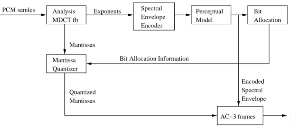
2.2 The encoding procedure of Dolby AC-3 coding system. . . 11

2.3 The principle of Psychoacoustic Masking [1]. . . 12

2.4 The decoding procedure of Dolby AC-3 coding system. . . 13

2.5 The encoding procedure of MPEG-2 AAC coding system. . . 14

2.6 The decoding procedure of MPEG-2 AAC coding system. . . 15

2.7 Modified AAC encoder in MAACKLT multichannel audio compression al-gorithm [2]. . . 16

2.8 The proposed decoder in MAACKLT multichannel audio compression algo-rithm [2]. . . 17

2.9 The main framework of Binaural Cue Coding [3]. . . 17

2.10 The psychoacoustic parameters’ synthesis scheme in the decoder of Binaural Cue Coding [4]. . . 17

2.11 The newer automobiles have at least five loudspeakers and a subwoofer, which, compared to home environments, are located in a better configuration. 19 3.1 M-channel filter bank. . . 22

3.2 (a) Downsampling and (b) Upsampling Operations. . . 22

3.3 Polyphase Decomposition for M=3. . . 24

3.4 Analysis filter bank. (a) direct implementation (b) polyphase realization. . 25

3.5 Synthesis filter bank. (a) direct implementation (b) polyphase realization. . 26

3.6 (a) Two-channel filter bank (b) Signal spectra with aliasing . . . 28

3.7 Regular tree-structured filter banks. . . 36

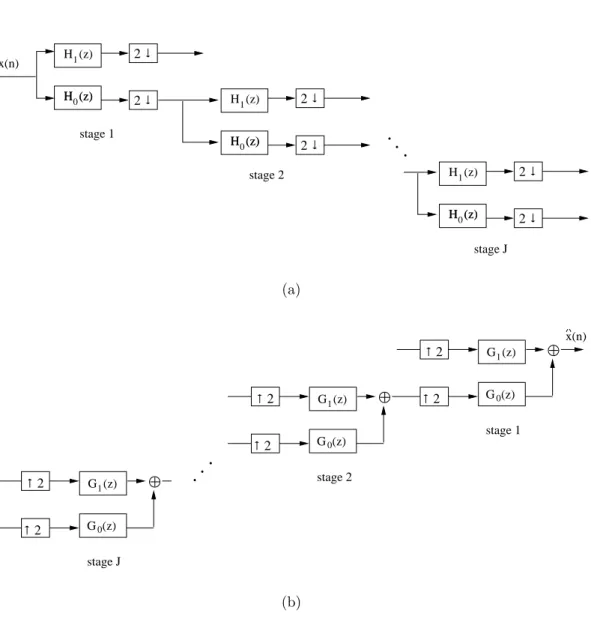
3.8 (a) Analysis (b) Synthesis Octave-band tree structure with J stages. . . 37

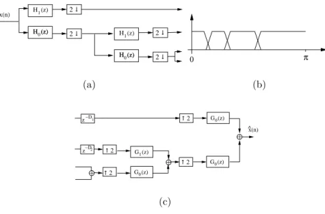
3.9 (a) Analysis (b) Synthesis Octave-band tree structure filter bank and (c) the corresponding frequency response. . . 38

3.10 M-channel filter bank in polyphase structure. . . 38

3.11 Idealized frequency response of the DFT filter bank. . . 40

(20)

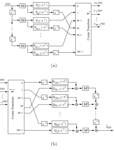
3.13 Modified DFT filter bank [5]. . . 42

3.14 (a) Analysis and (b) Synthesis Cosine Modulated filter bank with critical subsampling. . . 43

3.15 Kaiser window for window lengthn= 10 andα= 0.5, 1, 2, 4, 8, 16 (obtained from http://en.wikipedia.org/wiki/Kaiser window). . . 47

3.16 KBD window function for window length n = 100 and α = 0.5, 2, 8, 32 (obtained from http://en.wikipedia.org/wiki/Kaiser window). . . 47

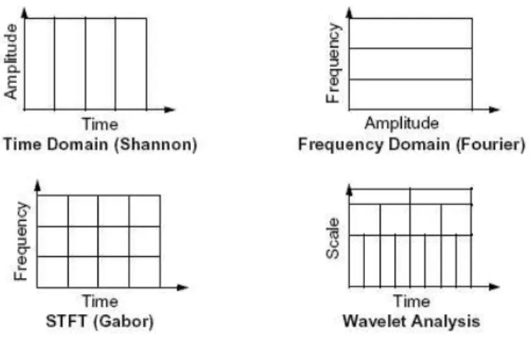
4.1 Wavelet Analysis contrary to other analysis techniques. . . 50

4.2 A Dirac pulse at t=t0 and its region of influence (a) for CWT and (b) for STFT [6, p. 20]. . . 51

4.3 Morlet Wavelet in time domain. . . 54

4.4 Octave-band analysis and synthesis filter bank [5, p. 222]. . . 55

4.5 Haar wavelet and scaling function [5, p. 230]. . . 57

4.6 Some members of the Daubechies family. . . 58

4.7 Scaling function, wavelet and their duals of Biorthogonal Wavelets, used in FBI fingerprint compression Standard [5, p. 251]. . . 59

4.8 Symlets Wavelets. . . 60

4.9 Mexican Hat Wavelet. . . 61

4.10 Meyer Wavelet. . . 61

5.1 AR analyzer with delayed inputs u(n−1), u(n −2), . . . , u(n−M) and parameters a1, a2, . . . , aM. . . 64

5.2 Forward Linear Predictor of order M, with tap inputsu(n−1), . . . , u(n−M) and linear prediction coefficientsw∗ 1, . . . , wM∗ . . . 68

5.3 The forward prediction error-filter, which uses the inputsu(n), u(n−1), . . . , u(n− M) to produce the error eM(n). . . 69

5.4 (a) A forward prediction error-filter of order M and (b) the corresponding autoregressive model. . . 71

5.5 (a) The spectrum of a signal with linear prediction coefficients at 210, 1280, 2320, 2720 and 3180 Hz and (b) the corresponding poles,whose angles θi, (i= 1, . . . ,4) with the horizontal axis are the LSF’s. . . 74

6.1 The representation of a GMM with M components. The unknown probabil-ity densprobabil-ity function g(x) of a random vectorxis given as the weighted sum of M Gaussian component densities N(x;µx i,Σxxi ) with mixture weights p(ωi), i= 1, . . . , M. . . 76

(21)

LIST OF FIGURES xxi

7.1 Consider a microphone signal M1, which can be seen as the convolution of its spectral envelopes1 and the residual signale1. Then, the residuale1 will contain the same harmonics as M1, but their amplitudes will have almost flat shape in the frequency spectrum. . . 89 7.2 If the AR vector could capture the exact envelope of the spectrum of

mi-crophones’ M1 and M2 recordings, the two residual signals e1 and e2 would have flat magnitude with exactly the same frequency components and they would resemble each other. Thus, they are almost equal in the frequency domain. . . 90 7.3 Every recording is decomposed into M subband signals. For each signal

we compute its spectral envelope, except from the subbands of the first recording, where we compute the residual signal, too. Then, we code and transmit all the envelopes with the residual of the first recording. . . 91 7.4 Normalized Mutual Information between the residual signals from the

ref-erence and target recordings as a function of the number of bands of the filter bank, for various filter orders. The increase of the filter order results in better separation of the different bands in frequency domain and thus in better modeling of the spectral envelopes. The latter is very important fea-ture, since it leads to more relevant residual signals, which in turn increases NMI. . . 94 7.5 Results from the 5-grade scale DCR-based listening tests, where graphical

representations of the 95% confidence interval are shown (the x’s mark the mean value and the two horizontal lines indicate the confidence limits). These results show clearly that the resynthesized signals are of high quality (similar to the quality of the original recording) and the model does not seem to introduce any serious artifacts. . . 96 8.1 The proposed Multiscale Source/Filter Model. . . 100 8.2 The modeling and coding procedure of (a) the first recording and (b) the j

recordings (j = 2, . . . , N), in the special case where a wavelet filter bank of W layers is been used. . . 100 8.3 Every layer from the wavelet decomposition is segmented into a series of

k short-time overlapping frames using a sliding Hamming window and AR analysis is applied in each frame. The spectral envelopes are modeled as LPC’s, which are converted in LSF’s. (a) In Layer 1, LSF’s are quantized and transmitted together with the residual signals while (b) in Layer j (j = 2, . . . , M) only the quantized LSF’s are transmitted. . . 102

(22)

8.4 Quantization scheme among clusters. . . 104 8.5 The logarithmic compression function c(x) = 1

2(1 +erf(x/

√

6)). . . 104 8.6 Overall Quantization scheme. . . 106 8.7 The reconstruction of the initial recordings at the receiver. . . 106 8.8 Results from the 5-grade scale DCR-based listening tests for the coding

(23)

Chapter 1 Introduction

During the last decade a revolution is taking place in the field of sound reproduction. Stereophonic audio is progressively being commercially substituted by multichannel audio. Audio reproduction systems with 5 or even 7 channels around the listener and 1 or 2 channels for low frequency sounds are becoming more and more popular. This increase of the audio channels, both at the capturing and rendering sides, leads to the creation of more realistic audio recordings that immerse the listener into the acoustic scene. The most prevalent configuration is the so-called“5.1 channels”. It was introduced in the film industry1 _{and tends to be the standard in home theatre systems.}

In the long run, multichannel audio reproduction systems are expected to be replaced by systems that immerse the listener into a virtual acoustic scene. The difference lies in the number of reproduction channels and in their way of placement (e.g. placing the listener in a sphere of loudspeakers). However, the main objective is the creation of an interactive scene, where the listener is not simply a passive receptor but can alter the acoustic scene depending on his needs.

These systems will allow the listener to modify his environment in real time and with the highest possible realism. For example, he will have the opportunity to virtually experience a live concert in the Boston Symphony Hall, through live audio and video streaming of the performance. Immersive Audio virtual rendering systems will also allow the remote collaboration of musicians. For example, musicians that are geographically distributed will have the opportunity of giving a common concert, while being in different locations. The audience can also be in different places, while they will have the sense of being in a specific concert hall, selected by the virtual concert’s organizer. The connection of the musicians and the audience will take place through the Internet.

There are several immersive audio systems’ applications of great importance, whose

1_{For more information about the first steps of multichannel audio the interested reader is referred to}

(24)

experimental implementation is allowed by todays’ technology. However, it is difficult to be implemented outside the laboratory’s conditions. For example, the IMSC2 _Laboratory captured the New World Symphony’s performance of Copland’s Symphony, using multi-channel audio methods and high definition video, and capturing the acoustics of Miami Beach’s Lincoln Theatre. The concert was stored on an IMSC server in Arlington and streamed to the campus of the University of Southern California in Los Angeles during the performance event. A 10.2 channel Immersive Audio system was installed in Bing Theatre to render the sound for the live audience as if they were at the Lincoln Theater on the original night of the performance. In this demonstration, the only constraint was the required bit rate; special networks were used with bit rate in the order of GBits/sec. Besides the fact that this kind of applications is impossible to be implemented in current Internet conditions, the implementation of virtual applications adds more constraints with regard to the required transmission bit rates.

1.1 Motivation

The augmentation of audio channels, which was occurred in the passage from stereo-phonic to multichannel audio, gives rise to a very important issue, that is how to efficiently record, store and transmit this amount of audio channels over the current Internet infras-tructure and wireless networks. This issue gained the interest of the research community and many compression techniques have been proposed in order to give efficient solutions in the issues of low data rate, low complexity and error manipulation. Consequently, multichannel audio compression algorithms have been developed which not only reduce the intra-channel redundancies, but the inter-channel redundancies as well. Some pop-ular methods of the latter is the Mid/Side Coding [7, 8, 9, 10], Intensity Stereo Coding [11, 10, 12, 13] and KLT-based methods [2].

Although the multichannel audio coding algorithms mentioned in the previous para-graph result in reduction of the data rates required by the original recording, they still remain highly demanding for many practical applications when the available channel band-width is low. This is especially important given the fact that many multichannel audio systems require even more than the 5.1 channels of currently popular standards, and thus even higher data rates. In recent years, the concept of Spatial Audio Coding has been in-troduced, with the objective of further taking advantage of inter-channel redundancies in multichannel audio recordings. Under this approach, the objective is to decode a (stereo or mono) channel of audio using some additional (side) information, so as to recreate

2_{Integrated Media Systems Center (IMSC) Laboratory of the University of Southern California (USC),}

(25)

Chapter 1. Introduction 3

the spatial rendering of the original multichannel recording. The side information is ex-tracted during encoding; in the most popular implementation of this approach, Binaural Cue Coding (BCC) [14, 3], the side information contains the inter-channel level difference, time difference, and correlation. The resulting signal contains one full channel of audio (downmix), along with the side information with bit rate in the order of few KBits/sec per channel.

Multichannel audio recordings are made using a large number of microphones in a venue, resulting in numerous microphone signals. These are then mixed in order to create the final multichannel audio recording. In many applications it would be desirable to transmit the multiple microphone signals of a performance, before those are mixed into the (usually much smaller number of) channels of the multichannel recording. This would allow for remote mixing of the multichannel recording, which is an important aspect for many applications in the music industry. Remote collaboration of geographically distributed musicians is a field of great significance with extensions to music education and research. Current experiments have shown that high data rates are needed so that musicians can perform and interact with minimal delay [15]. Remote mixing in the client side would also enable the user to interact with the music in an unparalleled fashion, allowing him to create his own music by mixing sounds as he pleases.

In this thesis, we propose a source/filter model for multichannel audio recordings that can be utilized for revealing the underlying inter-channel similarities. Our model consists of the filter part that corresponds to the specifics of each microphone information, and the source part that contains mostly the inter-channel similarities. Using the appropriate filter for each channel and the source part of only one of the microphone signals, we can resynthesize a high quality approximation of each channel. The filter part of each channel need only be encoded, requiring few KBits/sec/channel for high quality coding (along with one full audio channel); this part can be used to decode the multiple channels at the receiving end. Thus, the model achieves low bit rates for transmission of the multiple microphone signals of a music performance. This is important, since our method allows the transmission of multichannel audio signals through low bandwidth channels such as the current Internet infrastructure or wireless networks for broadcasting.

The methods proposed in this thesis are tailored towards the transmission of the various microphone signals (stem recordings) of a performancebefore they are mixed into the final multichannel signal. The algorithm can handle a large number of microphone signals that needs to be transmitted and can be applied to applications such as remote mixing and distributed performances. Our innovative approach relaxes the current bit rate constraints of these applications, allowing their widespread usage. Our method has the same objective with Spatial Audio Coding, i.e. to reduce a multichannel recording into one full audio

(26)

channel and some side information of the order of few KBits/sec per channel. However, it should be viewed as a generalization of BCC. In BCC, the side information can be used to recreate the spatial rendering of the various channels. In our method, the side information can theoretically (as we widely explain in the next chapters) recreate theexact microphone signals of the multichannel recording.

Finally, in our methodology, we propose a tradeoff between the accuracy andobjectives

of the final multichannel recording. We propose that it is possible to achieve low data rates by substituting some microphone signals with others, which, although they are different acoustically, they however retain the “objectives” of the initial recording. By the term “objectives” we refer to the aesthetic reason for a particular microphone placement (e.g. a microphone might be placed close to the chorus of an orchestra for placing emphasis on this part of the orchestra). With our algorithm, we attempt to resynthesize the recording of this “chorus microphone signal” using another microphone signal of the same performance (e.g. from a microphone placed close to the violins). The resynthesized signal can be of very good quality and might sound as if it was recorded with a microphone placed close to the chorus albeit different when compared to the actual “chorus microphone signal”. This is the case when the new signal retains the “objectives” of the recording, with a loss of “accuracy” (i.e. the new recording does not sound the same as the original recording). We claim that with our model it is possible to achieve low data rates, good audio quality, and retain the sense of realism, without significant sacrifices regarding the accuracy of the multichannel recording. The performance of the proposed model is verified by objective and subjective measures. The current model was presented in [16]

1.2 Structure of the thesis

The present thesis deals with the issue of Multichannel Audio Modeling and Coding and it is organized as follows: In Chapter 2, we describe the architecture of the most common used coding systems for multichannel audio; the Dolby AC-3 and the MPEG-2 AAC. We also present an algorithm similar to AAC, the MAACKLT, which proposes a new technique related to the reduction of inter-channel redundancies and a recent development in the concept of Spatial Audio Coding, called Binaural Cue Coding (BCC). In the next four chapters (Chapter 3 to 6) we discuss some fundamental theoretical issues, which contribute in the plenitude of the thesis and they are used in the implementation of the proposed method.

In Chapter 3, we present the basic theory regarding filter banks and we describe some popular filter banks such as QMF, DFT, MDFT and MDCT. Some of these filter banks have been implemented in order to improve the modeling performance of our algorithm. In

(27)

Chapter 1. Introduction 5

Chapter 4, we continue the theoretical analysis, examining the framework of wavelets. We begin with the definitions of Continuous and Discrete Wavelet Transforms and we describe some of the most frequently used wavelet families (Morlet, Haar, Daubechies, Symlets and more). In Chapter 5, we study two fundamental models in Autocorrelation Analysis; the Autoregressive Model and Linear Prediction Model. We close this chapter with the description of Line Spectral Frequencies (LSF’s) coefficients that are widely used in the proposed model. In Chapter 6, we present the Gaussian Mixture Model (GMM) and the Karhunen Lo`eve Transform, which are combined in our method to model and decorrelate the LSF’s of the multichannel signals. In Chapter 7, we propose a novel source/filter model for the transmission of multichannel audio signals, which takes advantage of the redundancy among the channels in order to achieve low data rate requirements. In particular, we begin with a brief description of how multimicrophone recordings for multichannel rendering are made, we continue with the description of the proposed method and we conclude with some modeling results, such as distortion measurements and statistical treatment of experimental data. In Chapter 8, we extend the use of the the speech source coding scheme of [17], in multichannel audio recordings. In this scheme, an optimal parametric vector quantizer for speech LSF’s is described, which has been applied in our source/filter model and we proceed to the results of the coding algorithm’s implementation. Finally, in Chapter 9, we conclude with remarks and we propose some future research directions.

(28)

(29)

Part I

(30)

(31)

Chapter 2 Background

2.1 Introduction to Multichannel Audio

Today, the majority of audio recordings used in the fields of information, entertainment, multimedia and so forth, are two channel presentations (stereo sound format). Despite the dominance of stereo, recently another audio format appeared, known as the “multichannel audio” or “surround sound” format. In the latter, several audio channels are recorded and mixed in order to recreate the spatial realism of the recording venue. Multichannel audio can immerse the listener into the acoustic scene, which is not possible to achieve by stereo music.

One of the most popular surround systems is the so-called “5.1 channels”, which refers to a format that uses five channels of full frequency sound and one subwoofer channel (“.1” designation) for low frequency effects (LFE), below 120 Hz. The needed bandwidth for the low frequency channel is very small compared to the rest five channels. The setup of the speakers that reproduce the channels’ signals are depicted in Fig. 2.11_.

Compared to the previous formats, in multichannel audio the amount of information needed to represent the audio signals is increased, which results in an imperative need to efficiently manipulate this information in order to store or transmit it. Therefore, many compression algorithms have been proposed, which represent the audio signals in a way that after decoding, the reproduced sound is very similar to the original, while achieving low data rates. The most dominant algorithms are implemented in two popular coding systems; the Digital Audio Compression Standard AC-3 of Dolby Laboratories and the Advanced Audio Coding (AAC) of MPEG. Other relevant algorithms are MAACKLT proposed in [2] and Binaural Cue Coding (BCC) [14, 3, 4]. In the next section we will describe these algorithms, trying to examine their strong points.

(32)

Figure 2.1: The setup of the speakers in “5.1 channels” surround system.

2.2 Multichannel Audio Coding Systems

2.2.1 Dolby AC-3

A very popular algorithm for high-quality audio compression is Dolby AC-3, which is also known as Dolby Digital or Dolby SR·D, has been developed by Dolby Laboratories at late 1980’s. It has both stereophonic and five-channel versions, while its data rates range from 32 to 640 kbps. In the “5.1 channels” case, the minimum achieved data rate for high quality audio is 382 kbps.

The encoding procedure of AC-3 coding system is depicted in Fig. 2.2. Overlapping blocks of 512 Pulse Code Modulation (PCM) time samples of an audio signal are multiplied by a Kaiser-Bessel Derived (KBD) analysis window and are modeled by the analysis part of a perfect reconstruction Modified Discrete Cosine Transform (MDCT) filter bank2_{. The} resultant frequency coefficients are represented as a binary exponent and a mantissa. The exponent encoder is a procedure, which exploits the MDCT coefficients redundancies that occur in time and frequency domain and estimates the signal spectrum known as spectral envelope. The mantissa quantizer groups MDCT coefficients in blocks, while the maximum of each block is quantized as an exponent proportional to the left shifts required until overflow. In the next step of encoding, the spectral envelope is used in the bit allocation routine. This routine evaluates the bits that will be used for the encoding of each mantissa and determines the prospective bit rate. Finally, the signal spectrum along with the quantized mantissas are combined into AC-3 frames, which are transmitted to the receiver.

2_{More information related to MDCT filter bank and window functions can be found in subsections 3.8}

(33)

Chapter 2. Background 11 Spectral Envelope Encoder Perceptual Model Bit Allocation Mantissa Quantizer Encoded Spectral Envelope Quantized Mantissas

AC−3 frames Encoded

Bit Stream PCM samles _Analysis

MDCT fb

Exponents

Mantissas

Bit Allocation Information

Figure 2.2: The encoding procedure of Dolby AC-3 coding system.

At this point we mention that Dolby AC-3 is enhanced with psychoacoustic analysis, exploiting knowledge of the properties of the human auditory system (in particular, the spectral and temporal masking effects of inner ear). The principle of audio masking is illustrated in Fig. 2.3. The signal component at 1 kHz, distorts and raises the masking threshold which defines the level that other signal components must exceed in order to be audible. If a second audio component is present at the same time and close in frequency to the first, then for the second component to be perceived by the ear, it must be at a higher level than it would otherwise need to be if present only on its own; otherwise it is masked by the first signal. Essentially, the system codes only audio signal components that the ear will hear and discards any audio information that the ear will not perceive, according to the psychoacoustical model.

Specifically in AC-3, (see Fig. 2.2), the coefficients of the spectral envelope are entered into a perceptual model, which estimates the masked threshold of each frame. This model exists only at the encoder, is not inverted to the decoder and it determines the most suitable (for the audio data) set of perceptual model parameters. After several threshold calculations in a rate control routine, these parameters result to a fixed form and they are transmitted to the decoder.

The encoding algorithm of AC-3 has some extra functions as well. A frame header is specified, which determines the bit-rate, the number of channels, the sampling frequency and more information necessary for the retrieval of the original bit stream at the decoder. Error detection functions are also inserted, which allow the decoder to make sure that the data are error free. The spectral resolution of the analysis MDCT filter bank can dynami-cally vary, adapting to the features of the audio blocks. Finally, the original channels may be coupled at high frequencies at the coding procedure (this technique is also known as intensity coding) [11, 10], in order to accomplish a more efficient coding approach. In chan-nel coupling the properties of spatial hearing are exploited and the main idea is to transmit only one spectral envelope (instead of two or more) from independent channels together

(34)

Figure 2.3: The principle of Psychoacoustic Masking [1].

with some side information, which is used in the decoder for recovering the individual envelopes.

On the other hand, the decoding portion of AC-3 system is mainly the inverse of the corresponding encoding, as it is shown in Fig. 2.4. The encoded bit stream is re-ceived, synchronized, checked for transmission errors and decomposed into spectral en-velopes and quantized mantissas. From bit allocation iterations, useful information for the de-quantization of mantissas is extracted. The spectral envelopes are decoded and transformed to exponents, which together with de-quantized mantissas are inserted to the synthesis MDCT filter bank, giving the original PCM time samples. In case where the transmitted channels were coupled in the encoding process, they must be de-coupled. Also, if the spectral resolution at the analysis filter bank has been assigned dynamically, it must be altered in the synthesis filter bank in the same manner. For more information on Dolby AC-3 the interested reader is referred to [11, 10, 12, 13].

2.2.2 MPEG-2 Advanced Audio Coding

MPEG-2 Advanced Audio Coding (AAC) is considered as the most powerful high-quality compression system for digital multichannel audio signals of the MPEG family, supporting up to 48 coded channels. It was developed in the early 1990’s and it achieves 320 kbps data rate for the “5.1 channels” surround system. The applications of AAC cover a very large range from multichannel broadcasting systems (Digital Audio Broadcasting (DAB), Digital TV Broadcasting, Music download services, Internet music streaming, In-ternet radio, Teleconferencing, Audio for games) to storage operations. The encoder and decoder of AAC system are shown in figures 2.5 and 2.6. Note that the decoder consists of the inverse encoding processes. The AAC is a scalable system, which offers three profiles [8, 9]:

(35)

Chapter 2. Background 13

Decomposition of AC−3 frames Syncronization, Error Detection and

Bit Allocation Spectral Envelope Decoder Encoded Spectral Envelope Quantized Mantissas MDCT fb Synthesis Mantissa De−Quantizer PCM samles Bit Allocation Information

Mantissas Exponents

Encoded Bit Stream

Figure 2.4: The decoding procedure of Dolby AC-3 coding system.

rates. All the tools depicted in Fig. 2.5 may be used, except the pre-processing tool and the memory/processing requirements are higher than low complexity profile (LCP). The decoder in the main profile can decode audio bit streams produced by the LC profile.

• Low Complexity Profile (LCP): In LCP, pre-processing and prediction tools are ex-cepted and the use of TNS (which will be discussed later) is restricted. The memory/ processing requirements are very low, while the high level of quality is retained.

• Scalable Sampling Rate Profile (SSRP): In this profile, a pre-processing tool is used, consisting of a polyphase quadrature filter (PQF), gain detectors and gain modifiers. The prediction tool is excluded, while TNS’s use is restricted. Lower complexity than MP and LCP and frequency scalable signals can be provided.

The MPEG AAC encoder, which is shown in Fig. 2.5, receives an audio signal and uses an appropriate window function together with an MDCT filter bank to decompose the input signal into subsampled spectral components. The window functions, which ensure the good frequency selectivity of the filter bank, vary dynamically with the signal’s characteristics. In particular, a switching between sine and KBD windows is allowed and an extra bit for every frame (signifying the window function) is transmitted to the decoder. Along with the decomposition in the frequency domain, an estimation of the current masking threshold is computed by the perceptual model. Rules from psychoacoustic field are applied for the threshold estimation and the resultant information is used in the quan-tizer, minimizing the audible quantization distortion.

After the analysis filter bank, the Temporal Noise Shaping (TNS) process is applied. In coding, many difficulties may occur due to the fact that quantization errors from one block are spread in time (extending in the order of few milliseconds) and are not effectively cut off by the masking threshold. This problem is known as the “pre-echo problem” and it is faced up by the TNS tool.

(36)

MDCT Filter Bank Pre Processing Intensity Coupling Prediction M/S Scale Factors Entropy Coding Perceptual Model Rate Control of previous frame Quantized Spectrum

Side Information Coding, Bitstream Formatting

Audio Stream AAC Encoded TNS Quantizer Input Signal

Figure 2.5: The encoding procedure of MPEG-2 AAC coding system.

As in Dolby AC-3, the intensity coding (or channel coupling) technique is used in AAC, together with Middle/Side (M/S) coding [7, 10], in order to eliminate the redundancies among channels. M/S technique (or “sum/difference coding”) is based on the evidence that the human ear at high frequencies (more than about 2 kHz) does not focus on the signal itself, but it mainly evaluates energy envelopes. Thus, in M/S two symmetric channels (e.g. arranged symmetrically on the listener’s left and right side) are not direct coded, but only their sum and their difference is encoded and transmitted.

The next step in AAC encoder is prediction, which exploits the fact that cascade frames’ spectral components (resulting from the spectral decomposition of the filter bank) are correlated, achieving redundancies reduction. Backward adaptive predictors are used and the quantizer is fed with the prediction error instead of the spectral components. However, the predictor is applied only in the case where a coding gain is guaranteed. For this reason an appropriate predictor control is applied. The latter activates the prediction procedure when coding gain can be achieved and transmits a small amount of predictor control information to the decoder. In a different case, prediction is deactivated.

The biggest data rate reduction is accomplished during quantization. Firstly, a non-uniform quantizer is applied to the spectral values, followed by Huffman coding. The number of bits used to code the quantized spectrum in Huffman procedure (12 Huffman codebooks are used), depends on the sampling frequency and the intended data rate. As mentioned before, the psychoacoustic model, which is similar to the one used in AC-3, contributes to the reduction of quantization distortion. Another tool, which amplifies the shaping of the quantization noise is the individual amplification of spectral coefficients’ groups, the so-called scale factor bands. The amplification information is stored in the scale factors and is transmitted to the decoder, while differential scale factors are Huffman coded. Finally, the quantized/coded coefficients and the control parameters (coded side information) are fed to a bit stream formatter, resulting to the final encoded bit stream of MPEG-2 AAC encoder.

At this point, we mention that the depicted (see Fig. 2.5) pre-processing part of the encoder is used only in the Scalable Sampling Rate Profile. It includes a PQF with four

(37)

Chapter 2. Background 15 Noiseless Decoding De−Quantizer Scale Factors M/S Prediction Intensity Coupling TNS MDCT Filter Bank Output Time Signal Audio Stream AAC Encoded Processing Post Side Information Decoding, Bitstream Formatting

Figure 2.6: The decoding procedure of MPEG-2 AAC coding system.

bandwidth output and at 48 Hz sampling rate it can give output bandwidth at 24, 18, 12 and 6 Hz. This part of the encoding process also consists of a gain control, which deals with the pre-echo problem as well as of gain controllers that control the amplitude of every PQF band. More information on the MPEG-2 AAC compression system can be found in [8, 9, 7, 10].

2.2.3 MAACKLT Multichannel Audio Compression Algorithm

Modified AAC with Karhunen-Lo`eve Transform (MAACKLT) is a compression system proposed in 2003, which is based on AAC algorithm and introduces two issues in multichan-nel coding [2]. Firstly, a novel inter-chanmultichan-nel decorrelation scheme is proposed, achieving a better coding gain. In particular, MAACKLT results in audio signals with better quality than AAC at the typical data rate of 64 kbps per channel. Secondly a quality-scalable encoding policy is suggested.

The encoder of this algorithm is shown in Fig. 2.7 and is a modified version of the corresponding AAC encoder. In Fig. 2.7 the shaded components show the novel parts, while the rest remain the same with AAC (see Fig. 2.5). One of the main differences compared to AAC is the use of Karhunen-Lo`eve Transform after the MDCT filter bank. After input signals’ transformation into the frequency domain, the KLT estimates the so-called decorrelated eigen-channel signals. The latter participate in the estimation of masking thresholds in the perceptual model. Overhead information that is related with KLT is added into the final bit stream. Another difference with AAC system is the fact that the M/S tool is disabled in MAACKLT. Since KLT results in independent eigen-channels with minimal correlation between any pair of channels, the M/S tool is not required. Finally, a prioritized eigen-channel transmission policy is applied, in order to achieve the quality scalability.

The decoding procedure of this algorithm is depicted in Fig. 2.8, where the encoded bitstream, the mapping information and the covariance matrices are extracted from the transmitted bit stream. If data loss occurs during the transmission, the eigen-channel concealment block is enabled to restore the lost data. The signals of the eigen-channels

(38)

Figure 2.7: Modified AAC encoder in MAACKLT multichannel audio compression algo-rithm [2].

are reconstructed from their compressed versions with the use of the decoder of the AAC main profile. The mapping information contributes to the restoration from a 16-bit dy-namic range of the decoded eigen-channel to their initial range. The inverse KLT uses the covariance matrices and reconstructs the multichannel blocks. Eventually, these blocks are combined to the desired multichannel signals. More detailed description of the MAACKLT can be found in [2, 18].

2.2.4 Binaural Cue Coding

In recent years, a new concept for efficient coding of multichannel audio signals has been introduced, calledSpatial Audio Coding. This approach takes advantage of the inter-channel redundancies in multiinter-channel recordings, maintains the backward compatibility with existing stereophonic decoders and achieves data rates close to those needed for stereo (or mono) transmission. The most popular development in coding of spatial audio is the Binaural Cue Coding (BCC), which is based on the parametric coding of multichannel signals using well-known parameters from psychoacoustics [14, 3, 4].

The main framework of BCC is illustrated in Fig. 2.9. In the BCC encoder, the input signalsx1(n), . . . , xC(n) are downmixed into a singlesum signal, while the most prominent

perceptually motivated parameters are extracted. In the psychoacoustic area, the inter-channel time difference (ICTD), level difference (ICLD) and correlation (ICC) have a well recorded history in describing the perception of the auditory spatial image. The latter parameters are evaluated between channel pairs (both in frequency3 _{and time domain) and} coded, constituting the BCC side information. The BCC side information together with the coded downmixed signal are transmitted to the receiver, where the decoder attempts

3_{ICTD, ICLD and ICC are estimated in the frequency domain using a Cochlear filter bank or a}

(39)

Figure 2.8: The proposed decoder in MAACKLT multichannel audio compression algo-rithm [2].

Figure 2.9: The main framework of Binaural Cue Coding [3].

to resynthesize the spatial image. Thereby, in the decoder thesum signal (see Fig. 2.10) is processed by a filter bank and spectral coefficients are estimated. The latter are combined with different delays (d1, . . ., dC) and different scale factors (ai, i = 1, . . . , C), and they

are re-correlated. The resultant signals are converted to the time domain by the synthesis part of the filter bank (IFB).

The bit rates achieved by BCC, range from 24 kbps to 64 kbps and the lower the bit rate the more is the BCC coding scheme at an advantage (compared to relevant algorithms). Finally, BCC has been included in the standardization of MPEG Surround System by the ISO/MPEG group [19] and in the experimental multichannel version of the popular MP3 compression format [20].

Figure 2.10: The psychoacoustic parameters’ synthesis scheme in the decoder of Binaural Cue Coding [4].

(40)

2.3 Areas of Applications

The following areas are some examples where multichannel audio is starting to appear.

Audio Broadcasting:

Today, most of the digital broadcasting systems provide interference-free reception and the potential for enhanced user services. However, due to the small channel bandwidth, the large cost of transmission equipment and radio broadcasting licenses the spread of these systems is limited. In the future, it is expected that the current radio programs will be supplemented by multichannel audio, pictures, texts and graphics, which will increase their information value and will motivate the users to make the transition from the traditional FM receivers to new digital receivers. In this scheme, multichannel audio meets its most promising application.

Despite the tremendous usage in home theatre surround systems, multichannel audio is not widely used in environments such as cars. This could be a very popular multichannel implementation, since many people in their cars listen to the radio. The newer automobiles have at least five loudspeakers and a subwoofer, which, compared to home environments, are located in a better configuration (Fig. 2.11). The listener in the car also, has a stable and predictable position regarding to loudspeakers, which provides a more realistic expe-rience of the music. Recently, mostly in the US, service providers of satellite radio such as Cirius and XM transmit their programs in multichannel format [21, 22].

Digital Television Broadcasting:

Currently, the majority of digital TV broadcasting services use the stereo audio format. On the other hand, the few Digital Video Broadcasting (DVB) systems, which provide surround sound, simulcast stereo and multichannel services. The latter though is contained in a separate data-stream, resulting in high bit rates and great operational complexity. The greatest challenge of multichannel systems applications is to establish these services to multichannel format with a small overhead in bit rate at the same transmitting signal, while maintaining stereo compatibility.

Internet Audio:

A few years ago, the usage of perceptual models in audio coding systems (such as MP3 of MPEG family and Dolby AC-3) led to a rapid development of Internet audio

(41)

Figure 2.11: The newer automobiles have at least five loudspeakers and a subwoofer, which, compared to home environments, are located in a better configuration.

and computer based audio. Nowadays, an experimental backward compatible extension of MP3 compression format is presented by the Fraunhofer IIS [20], which produce high quality 5.1-channel sound using novel coding schemes such as BCC. Such multichannel compression formats could be used in various ways. Many radio stations are streaming their program to the Internet. Due to the constrained transmission bandwidth they only use stereo or ever monophonic content. Thus, the streaming of multichannel audio through radio broadcasting material is a very challenging field.

Another possible service of surround sound, related to Internet, is music download and preview service. A number of commercial music download services are already available and work with success, using stereo sound. Additionally, many record companies and music companies (working with mail orders) would like to give the consumers the opportunity to listen a short time of their products even a low quality preview of their music songs. Such services could be implemented with multichannel audio coding systems, since scalability (for preview service) and high audio quality are provided.

(42)

(43)

Chapter 3 Filter Banks

3.1 Introduction to Filter Banks

In this chapter we study filter banks, which are structures of low pass, bandpass, and highpass filters, commonly used in signal processing applications, such as audio and image coding [23, 24, 5, 25, 26, 27, 28, 29]. Their popularity derives from the fact that they provide efficient implementations of signals decomposition and composition, emphasizing in prescribed spectral aspects of the original signal.

Figure 3.1 depicts a filter bank, which consists of M channels. The input signal x(n) is decomposed in M signals y0(m), y1(m), . . . , yM−1(m) using the passband fil-ters H0(z), H1(z), . . . , HM−1(z) and a downsampler of order N. By downsampling, we

ignore samples which are located in multiples of N and the sampling rate for each channel is reduced by N. The signals yi (i= 0, . . . , M −1) are called subband signals and the first

part of the depicted structure (up to these signals) is called analysis filter bank.

In order to reconstruct the original signal, we first apply an upsampler (of order L), we then pass the upsampled signals through M filters G0(z), G1(z), . . . , GM−1(z) and finally we add the resultant signals. In upsampling operation we insert zeros between the samples to recover the original sampling rate, while the following filters replace these zeros with meaningful values. The second part of the depicted structure is called synthesis filter bank. If the order of downsampler equals the order of the upsampler (N = L), the sampling is entitled as critical subsampling, since this order is the maximum factor for which we succeed the perfect reconstruction of x(n).

In the rest of this section, we begin with the definition of some fundamental issues in filter bank analysis and we continue describing some of the most frequently used filter banks.

(44)

... ... ... ... ... M−1 y (m) N N N H (z)₀ H (z)₁ H (z) H (z)M−1 G (z)M−1 0 1 G (z) G (z) + y (m)₁ y (m)₀ x(n) ^x (n) L L L

Figure 3.1: M-channel filter bank.

3.1.1 Sampling Operation

Downsampling:

This operation serves to reduce or to eliminate redundancies in the M subband signals. In Fig. 8.3(a) the following relationship holds

x0_{[n] =}_x[Nn]. _(3.1) In z-transform domain: X0(z) = 1 N N_X−1 k=0 X(W_NkzN1) whereW_N =e− j2π N (3.2)

where X0_{(z) is the z-transform of}_x0_[n].

Equation (3.2) for N = 2 becomes X0_{(z) =} 1

2(X(z

1

2) +X(−z12))

Upsampling:

This operation serves to recover the original sampling rate by inserting zeros between the

N x (n) x(n) (a) L x (n) x(n) (b)

(45)

Chapter 3. Filter Banks 23

samples. In Fig. 8.3(b) the following relationship holds

x0[n] =    x[n/L], n=kL, k∈Z 0, n 6=kL (3.3) In z-transform domain: X00(z) = X0(zL) (3.4) and for L= 2 : X00(z) =X0(z2) = 1 2(X(z) +X(−z))

3.1.2 Matrix Representations

In filter bank analysis we usually use matrix representations, because they are more con-venient and they also offer a compact way to describe filter banks. Below, we give the definitions of some important matrices and we describe their relation to the analysis and synthesis filters. Most of the following relations refer to a two-channel filter bank, but they can be generalized.

Analysis and Synthesis Matrices:

In order to express the two-channel filter bank in a compact matrix form, we define the Toeplitz matrix Hm(z) =   H0(z) H0(−z) H1(z) H1(−z)  _, _(3.5)

which is called analysis matrix and the matrix

Gm(z) =   G0(z) G1(z) G0(−z) G1(−z)  _, _(3.6)

which is known as synthesis matrix. Thus, the relation between the subband signals and the original signal is given in a matrix form by

yp(z2) =

1 2H

T

(46)

where xm(z) =  X(z) X(−z)  _, yp(z) =  Y0(z) Y1(z)  _. (3.8)

3.1.3 Polyphase Decomposition

A polyphase decomposition of a signal x(n) into M components is given by [27]:

X(z) = M_X−1 l=0 z−l_X l(zM), (3.9) where Xl(z)↔xl(n) =x(nM +l). (3.10)

An example of polyphase decomposition of a signal x(n) into three sub-signalsx0(n), x1(n), x2(n) is shown in Fig. 3.3. The aforementioned sub-signals are called polyphase components of

x(n) and if we interleave them, we can retrieve the original signal x(n).

Polyphase Representation of the Analysis Filter Bank:

If we consider the analysis filter bank shown in Fig. 3.4(a), the signalsy0(m) andy1(m)

(47)

Chapter 3. Filter Banks 25 H (z)₀ H (z)₁ H (z) 2 2 y (m)₀ y (m)₁ x(n) (a) 2 H (z)₀₀ 0 H (z)₁ H (z)₁₀ H (z)₁₁ 2 x (m)₀ _ _ x (m)1 + + y (m)₀ y (m)₁ z−1 x(n) (b)

Figure 3.4: Analysis filter bank. (a) direct implementation (b) polyphase realization. can be written as y0(m) = P n h0(n) x(2m−n) = P k h0(2k) x(2m−2k) +P k h0(2k+ 1) x(2m−2k−1) = P k h00(k) ¯x0(m−k) + P k h01(k) ¯x1(m−k) (3.11) and y1(m) = P n h1(n)x(2m−n) = P k h10(k) ¯x0(m−k) + P k h11(k) ¯x1(m−k) , (3.12) where h00(k) = h0(2k), h01(k) = h0(2k+ 1), h10(k) = h1(2k), h11(k) = h1(2k+ 1), ¯ x0(k) = x(2k), ¯ x1(k) = x(2k−1). (3.13)

are the polyphase components [5].

From equations (3.11) and (3.12) we conclude that we can implement the analysis fil-ter bank using the polyphase components (Fig. 3.4(b)). If we compare this polyphase implementation with the respective direct one (Fig. 3.4(a)) we observe that only the re-quired components are computed. Thus, efficient implementation with simple filter design is achieved, taking advantage of filter bank’s properties.

Equations (3.11) and (3.12) can be rewritten in matrix form and in the z-domain as

yp(z) = Hp(z)¯xp(z) (3.14)

(48)

yp(z) =  Y0(z) Y1(z)  _,_x_¯_p_{(z) =}  X0(z)¯ ¯ X1(z)  _, Hp(z) =   H00(z) H01(z) H10(z) H11(z)  _. (3.15)

Matrix Hp(z) is called the analysis polyphase matrix and Hik(z) is the kth polyphase

components of the ith _filter _H

i(z), where

Hi(z) =Hi0(z2) +zHi1(z2). (3.16)

It is obvious that polyphase decomposition is used for the signals as well for the filters of the filter bank.

Polyphase Representation of the Synthesis Filter Bank:

Let us now consider the synthesis part of a filter bank as depicted in Fig. 3.5, where (a) shows the direct implementation and (b) shows the polyphase realization of the filter bank. Respectively with the analysis polyphase matrix Hp(z), we define the synthesis polyphase

matrix Gp(z) by Gp(z) =   G00(z) G10(z) G01(z) G11(z)   _(3.17) where Gi(z) = Gi0(z2) +z−1Gi1(z2) (3.18)

The z-transform ˆX(z) of the reconstructed signal ˆx(n), in matrix representation is given

+

2 2 _^ x(n) y (m)₀ y (m)₁ G (z)1 G (z)₀ (a) y (m) 0 + + 2 2 + y (m) 1 z−1 00 01 0 1 11 G (z) G (z) G (z) G (z) (b)

(49)

Chapter 3. Filter Banks 27 by ˆ X(z) = h 1 z−1 i  G00(z2) G10(z2) G01(z2₎ _G11(z2₎    Y0(z2) Y1(z2)  _. _(3.19)

Note that the synthesis polyphase matrix and the last vector in equation (3.19) is in z2_{. This allows us to put filters} _G

ik(z), i, k = 0,1 before the upsampler and replace z2

by z in the implementation, as shown in 3.5(b). We can also observe a duality between the analysis and synthesis filter bank and that Gp(z) is a transpose of Hp(z), in indices

concept [24].

If we substitute equation (3.14), (3.15) and (3.17) in (3.19) we result in a relation between the z-transform of the output signal ˆx(n) and the z-transform of the input signal x(n): ˆ X(z) = h 1 z−1 i Gp(z2)Hp(z2)¯xp(z2). (3.20)

3.1.4 Perfect Reconstruction

When we say that a signal can be perfectly reconstructed by a filter bank, we mean that the output signal ˆx[n] is a copy of the input signal x[n] with no further distortion than a time shift and an amplitude scaling [5].

Below we give the constraints on the analysis and synthesis filter banks that ensure perfect reconstruction in direct, z-transform domain, matrix and polyphase form.

Direct Characterization:

If we consider the filter bank shown in Fig. 3.1, then an analysis filter bank is Perfect Reconstruction (PR) iff M_X−1 i=0 X n hi(Nn+n1)gi(−Nn+n2) = δ(n1−n2), ∀n1, n2. (3.21)

Correspondingly [23], a synthesis filter bank is PR iff

X

n

hi(L)gi(−Ln+n2) = δ(l)δ(i−j), ∀i, j ∈ {0,1, ..., M −1}. (3.22)

If the order of the downsampler equals the order of the upsampler (M = N), (where the sampling is called critical subsampling), equations (3.21), (3.22) are equal.

(50)

y (m)₀ y (m)₁ ’ ’ H (z)₀ H (z)₁ H (z) 2 2 + 2 2 y (m)₀ y (m)₁ x(n) G (z)0 x(n)^ G (z)1 (a) H (e )₁ jω H (e )₀ jω (b)

Figure 3.6: (a) Two-channel filter bank (b) Signal spectra with aliasing .

Z-transform domain:

In z-transform domain the general condition for perfect reconstruction is given by ˆ

X(z) = z−q_X(z) _(3.23)

where ˆX(z) is the z-transform of the constructed signal and X(z) is the z-transform of the original signal.

Let us now consider the two channel filter bank of Fig. 3.6(a). Further down we calculate the relation between the inputX(z) and the output ˆX(z).

ˆ

X(z) =Y₀0(z)G0(z) +Y10(z)G1(z). (3.24) However, Y0

i(z) (i= 0,1) can be represented with the use of equation (3.4) as

Y0

0(z) =Y0(z2), Y10(z) = Y1(z2). (3.25) Equation (3.25) combined with (3.2), is rewritten as

Y0(z2) = 1

2[H0(z)X(z) +H0(−z)X(−z)] Y1(z2) = 1

2[H1(z)X(z) +H1(−z)X(−z)]

(3.26)

The combination of (3.24), (3.25) and (3.26) yields the input-output relation: X(z) = 1

2[H0(z)G0(z) +H1(z)G1(z)]X(z) + 1

2[H0(−z)G0(z) +H1(−z)G1(z)]X(−z).

(3.27)

In equation (3.27), the first adding factor characterizes the transmission ofX(z) through a two-channel filter bank (Fig. 3.6(a)) and the second characterizes the aliasing

Multichannel Audio Modeling and Coding Using a Multiscale Source/Filter Model

Multichannel Audio Modeling and Coding

Using a Multiscale Source/Filter Model

(MSc. Thesis)

Kyriaki Karadimou

Heraklion

November 2005

Multichannel Audio Modeling and Coding Using a

Multiscale Source/Filter Model

Abstract

PerÐlhyh

EuqaristÐec

Contents

I

Theoretical Background

7

II

Multichannel Audio Modeling and Coding

83

III

Appendices

113

List of Tables

List of Figures

Chapter 1

Introduction

1.1

Motivation

1.2

Structure of the thesis

Part I

Chapter 2

Background

2.1

Introduction to Multichannel Audio

2.2

Multichannel Audio Coding Systems

2.2.1

Dolby AC-3

2.2.2

MPEG-2 Advanced Audio Coding

2.2.3

MAACKLT Multichannel Audio Compression Algorithm

2.2.4

Binaural Cue Coding

2.3

Areas of Applications

Chapter 3

Filter Banks

3.1

Introduction to Filter Banks

3.1.1

Sampling Operation

3.1.2

Matrix Representations

3.1.3

Polyphase Decomposition

+

3.1.4

Perfect Reconstruction