arXiv:2012.13468v1 [math.CO] 25 Dec 2020
Exponential Growth Constants for Spanning Forests on Archimedean Lattices: Values
and Comparisons of Upper Bounds
Shu-Chiuan Changa and Robert Shrockb
(a) Department of Physics, National Cheng Kung University, Tainan 70101, Taiwan and (b) C. N. Yang Institute for Theoretical Physics and Department of Physics and Astronomy
Stony Brook University, Stony Brook, NY 11794, USA
We compare our upper bounds on the exponential growth constantφ(Λ) characterizing the asymp-totic behavior of spanning forests on Archimedean lattices Λ with recently derived upper bounds. Our upper bounds on φ(Λ), which are very close to the respective values of φ(Λ) that we have calculated, are shown to be significantly better for these lattices than the new upper bounds.
I. INTRODUCTION
LetG= (V, E) be a graph, defined by its vertex and edge sets V and E, and denote n = n(G) = |V| and
e(G) =|E|as the numbers of vertices (= sites) and edges (= bonds) inG. An important problem in mathematics is the determination of the number of subgraphs of G
that satisfy a specified property, and, in particular, the asymptotic behavior of this number as n(G) → ∞. A spanning subgraph ofG, denotedG′, is a graph with the
same vertex set, V′ = V and a subset of the edge set
of G, E′
⊆ E. A forest is a spanning subgraph that does not contain any cycles. Given a graph G, let us denote the number of spanning forests in Gas NSF(G)
and the number of connected spanning subgraphs in G
as NCSSG(G). For many families of graphsG, NSF(G)
andNCSSG(G) grow exponentially rapidly as functions of
n(G) for largen(G), thereby motivating the definitions of corresponding exponential growth constantsφ({G}) and
σ({G}), φ({G}) = lim n(G)→∞[NSF(G)] 1/n(G) (1.1) and σ({G}) = lim n(G)→∞[NCSSG(G)] 1/n(G) , (1.2)
where{G} denotes then(G)→ ∞limit of the graphs in a given family. Recall that the degree ∆vi of a vertexvi in a graphGis the number of edges connecting tovi. A
graph with the property that all of its vertices have the same degree ∆ is termed a ∆-regular graph. To avoid unimportant complications, we restrict here to loopless graphs.
In Ref. [1] we calculated upper bounds on φ(Λ) and
σ(Λ), where Λ denotes the n(G) → ∞ limit of an Archimedean lattice graph. Here an Archimedean lat-tice is defined as a uniform tiling of the plane with one or more types of regular polygons, such that all vertices are equivalent, and hence is ∆-regular. In general, an Archimedean lattice Λ is identified by the ordered se-quence of regular polygons traversed in a circuit around any vertex [2, 3]:
Λ = (Ypai
i ), (1.3)
where thei’th polygon haspisides and appearsaitimes
contiguously in the sequence (it can also occur non-contiguously). There are three Archimedean lattices which each involve only a single type of polygon, namely honeycomb = (63), square = (44), and triangular = (36),
abbreviated as (hc), (sq), and (tri), respectively. The other Archimedean lattices are heteropolygonal, i.e., they involve more than a single type of polygon. Examples are (4·8·8), (3·6·3·6) (often called “kagom´e” (kag)), (33·42), and (3·3·4·3·4). With appropriate boundary
conditions, a finite section of an Archimedean lattice is a ∆-regular graph. The ∆ values for the Archimedean lattices range from 3 to 6. Our upper bounds were de-notedφu(Λ) andσu(Λ), where the subscriptustands for
“upper”. Our bounds are, to our knowledge, the best up-per bounds onφ(Λ) andσ(Λ) for these lattices. In [1] we also calculated lower bounds on these exponential growth constants, which are very close to the respective upper bounds, with fractional differences ranging from 10−4 to
10−2. This property enabled us to calculate quite
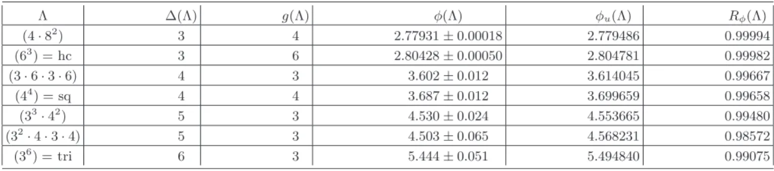
ac-curate approximate values of φ(Λ) and σ(Λ) for these lattices, which we denote here simply asφ(Λ) andσ(Λ). For each lattice Λ, our method made use of calculations of lower and upper bounds onφand σfor a sequence of infinite-width lattice strips of increasing widths. Our ap-proximate values were determined conservatively as the average of our lower and upper bounds on the widest strips with periodic transverse boundary conditions (to minimize finite-width effects). As we noted in [1], our upper bounds and approximate values forφ(Λ) andσ(Λ) are monotonically increasing functions of the vertex de-gree ∆ for the Archimedean lattices that we studied. In the following, we focus on our results for φ(Λ) in view of new general bounds in [4]. For reference, we list our upper bounds and values for φ(Λ) from [1] in Table I, together with the ratio of our (central) value ofφ(Λ) di-vided by our upper bound for each Λ, namely
Rφ(Λ) = φ(Λ)
φu(Λ)
. (1.4)
The fact that the ratiosRφ(Λ) for these lattices are very
close to unity shows how close our upper bounds are to being sharp. We found that our upper bounds onφ(Λ) andσ(Λ) approach limiting values more rapidly than our lower bounds, so that the true values of Rφ(Λ) are
ex-pected to be even closer to unity than the values listed in Table I, i.e., the respective upper bounds are even closer to being sharp for these lattices.
LetG∆denote the set of all ∆-regularn-vertex graphs.
Recently, in Ref. [4], Bob´enyi, Csikv´ari, and Luo (BCL) presented upper bounds on the supremum over allG ∈ G∆of the quantity [NSF(G)]1/n(G),
f∆= supG∈G∆[NSF(G)]1/n(G) . (1.5)
The upper bounds reported in [4] do not depend onn(G), so they also apply in then(G)→ ∞limit, yielding upper bounds onφ, which we denote as
φu,BCLi(∆) = lim
n(G)→∞supG∈G∆[NSF(G)]
1/n(G), (1.6)
where the subscriptiwill label the specific BCL bounds. It is of considerable interest to compare the BCL up-per bounds with our upup-per bounds and values for the Archimedean lattices that we considered in [1]. We per-form this comparison in the present paper.
II. COMPARISON OF UPPER BOUNDS ONφ(Λ) We first recall a general upper bound for any set of spanning subgraphs, including spanning trees, spanning forests, and connected spanning subgraphs. In the con-struction of a spanning subgraph, there is choice for each edge ofG, namely whether it is present or absent. Since this is a two-fold choice for each edge, it follows that the number of spanning subgraphs ofGis
NSSG(G) = 2e(G). (2.1)
This is an upper bound for any specific subclass of spanning subgraphs. Hence, in particular, for spanning forests,
NSF(G)≤NSSG(G). (2.2)
Since for ∆-regular graphsG∈ G∆,
e(G) = n(G)∆
2 , (2.3)
it follows that for these ∆-regular graphs,
f∆≤2∆/2, (2.4)
and hence, in the limitn(G)→ ∞,
φ({G∆})≤2∆/2 . (2.5)
Before comparing our upper bounds on φ(Λ) to the
n(G) → ∞ limits of upper bounds recently derived in [4], we mention some previous bounds. After early work [5], Ref. [6] obtained the upper limit
φ(sq)≤3.7410018 (2.6)
Before our work in [1], the best upper bound onφ(sq) was from Mani, in Ref. [7], namely
φ(sq)≤3.705603. (2.7) In [1] we derived the upper bound
φ(sq)≤3.699659. (2.8) As we noted, our upper bounds on φ(Λ) for this and the other Archimedean lattices that we studied are, to our knowledge, the best upper bounds onφ(Λ) for these lattices. Our results in [1] were part of a general pro-gram of calculating bound on, and values of, exponen-tial growth constants for various classes of subgraphs on Archimedean lattices [8–10].
A first upper bound proved in [4] is
NSF(G)≤ Y
vi∈V
(∆vi+ 1). (2.9) The special case of this bound for a ∆-regular graphG
is
f∆≤∆ + 1, (2.10)
which also applies in the limit asn(G)→ ∞as
φ({G∆})≤∆ + 1. (2.11)
We denote the right-hand side of (2.11) as
φu,∆,BCL1(∆) = ∆ + 1. Generalizing ∆ from
posi-tive integral values to posiposi-tive real values, we find that the upper bound (2.5) is more stringent than (2.11) if ∆<5.3197.
A second upper bound for ∆-regular graphs discussed in [4] is f∆≤fu,BCL2(∆) , (2.12) where fu,BCL2(∆) = ∆ + 1 η(∆) ∆−1 ∆−η(∆) ∆−22 , (2.13) with η(∆) =(∆ + 1)(∆ + 1− √ ∆2−2∆ + 5 ) 2(∆−1) . (2.14)
(See also [11] for related work.) Since this bound applies uniformly for any n(G), it also applies to the limit as
n(G)→ ∞:
φ(Λ)≤φu,BCL2(∆), (2.15)
whereφu,BCL2(∆) =fu,BCL2(∆). We list below the
an-alytic expressions of the upper bound φu,BCL2(∆) and
the corresponding numerical values (given to the indi-cated number of significant figures) for the values of ∆ that are relevant for comparison with our bounds:
φu,BCL2(2) = 3 + √
5
φu,BCL2(3) = 2 11 + 8√2 7 1/2 = 3.5708109 (2.17) φu,BCL2(4) = 35 + 13√13 18 = 4.5484537 (2.18) φu,BCL2(5) = 4√2 (27 + 7√5)p1 + 3√5 121 = 5.5361833 (2.19) and φu,BCL2(6) = 791 + 58√29 169 = 6.52863644. (2.20) An upper bound given in Ref. [4] for 4-regular graphs G4, which we label BCL3, is:
f4≤3.994, (2.21)
and again, since this is independent of n(G) for G ∈ G4, it implies, in then(G)→ ∞limit, the upper bound
φ({G4})≤φu,BCL3(4), where
φu,BCL3(4) = 3.994. (2.22)
Finally, Ref. [4] presented slightly stronger upper bounds on f∆ for ∆-regular graphs G∆ with ∆ in the
interval 5 ≤ ∆ ≤ 9. As before, their upper bound for each ∆ makes no reference to n(G), so that it implies the same bound for then(G)→ ∞ limit of a ∆-regular graph for ∆ in this interval 5≤∆≤9:
φ(Λ)≤φu,BCL4(∆) for 5≤∆≤9 . (2.23)
In the two cases with ∆ = 5 and ∆ = 6 rele-vant for Archimedean lattices, these upper bounds are
φu,BCL4(5) = 5.1965 and φu,BCL4(6) = 6.3367 [4].
We list the numerical values of the BCL upper bounds on φ(Λ) in Table II for the ∆ values that occur for Archimedean lattices, namely ∆ = 3,4,5,6. As is ev-ident, for a given ∆, these BCL upper bounds are all less stringent than the upper bounds that we derived on
φ(Λ) for the ∆-regular Archimedean lattices Λ in [1]. This comparison is made for the full range of ∆ val-ues on Archimedean lattices, namely ∆ = 3, 4, 5, 6. For the case of ∆ = 2, we recall the elementary re-sult that NSF(Cn) = 2n−1 and hence, in the n → ∞
limit,φ(C∞) = 2. This saturates the upper bound (2.5),
but is less than the upper bounds φu,BCL1(2) = 3 and
φu,BCL2(2) = (3 + √
5)/2 = 2.6180.
Although the BCL bounds onφdepend only on ∆, our upper boundsφu(Λ) and also the values ofφ(Λ) that we
calculated in [1] enable us to investigate the dependence on girth g(Λ) for lattices with the same value of ∆. As one can see from Table I, two such comparisons can be made for Archimedean lattices: (i) the (63) =hc and (4·
82) lattices both have ∆ = 3, but the girthg(hc) = 6 is
larger than the girthg((4·82)) = 4, andφ(hc) is slightly
larger thanφ((4·82)); (ii) the square and kagom´e lattices
both have ∆ = 4, but the girthg(sq) = 4 is larger than the girth g(kag) = 3, and φ(sq) is slightly larger than
φ(kag). Note that the uncertainties in our numerical determination of the values ofφ(Λ) for the Archimedean lattices are sufficiently small that they are negligible for these comparisons.
In earlier work preceding [1, 9, 10], we had calcu-lated values of exponential growth constants for a va-riety of families of lattice strip graphs of various lat-tices with a range of finite widths and with arbitrar-ily great length (e.g., [14]-[19]). We found that for a given type of lattice strip graph, in the infinite-length limit,φis a monotonically increasing function of the strip width. For the smallest widths, one obtains simple alge-braic expressions for these exponential growth constants. For example,φ has the following values for the infinite-length limits of the given strips: φ = 1 +√3 = 2.732 and φ = (√7 +√15)/2 = 3.259 for the transverse width Lt = 2 strips of the square lattice with free (F)
and periodic (P) tranverse boundary conditions (BCt);
φ= 2 +√2 = 3.414 andφ= [(23 +√505)/2]1/2= 4.768
forLt = 2 strips of the triangular lattice with F and P
BCt, etc.
While our upper bounds φu(Λ) are better than the
BCL upper bounds in [4] for the Archimedean lattices Λ that we studied, the BCL upper bounds are still valu-able, since they apply for any ∆-regular graphs, not just Archimedean lattices. In future work it would be of in-terest to search for ∆-regular families of graphs for which
f∆ and/or limn(G)→∞f∆ lie closer to the upper bounds
given in [4].
Acknowledgments
This research was supported in part by the Taiwan Ministry of Science and Technology grant MOST 109-2112-M-006-008 (S.-C.C.) and by the U.S. National Sci-ence Foundation grant No. NSF-PHY-1915093 (R.S.).
Appendix A: Some Background from Graph Theory
In this appendix we briefly review some background from graph theory, in particular, a connection ofNSF(G)
and NCSSG(G) with evaluations of the Tutte
polyno-mial. As in the text, let G = (V, E) be a graph de-fined by its vertex and edge sets V and E. Further, let
n=n(G) =|V|,e(G) =|E|, k(G), and c(G) denote the numbers of vertices, edges, connected components, and linearly independent cycles inG, respectively. The Tutte polynomial of a graphG, denoted T(G, x, y), is defined as
T(G, x, y) = X
G′⊆G
(x−1)k(G′)−k(G)(y
whereG′is a spanning subgraph ofG(see, e.g., [12, 13]).
The numbers of spanning forests and connected spanning subgraphs are evaluations of the Tutte polynomial:
NSF(G) =T(G,2,1) (A2)
and
NCSSG(G) =T(G,1,2). (A3)
For a general graph G, the calculation of NSF(G) and
NCSSG(G) are♯P hard [20]. This is why it is useful to
have bounds on these quantities, and also on the corre-sponding exponential growth constants.
A remark is in order here concerning graphs with loops. Recall that a loop is an edge that connects a vertex back to itself. The reason that we restrict to loopless graphs in our work is that if one allows loops, then one loses a connection between the vertex degree of a ∆-regular graphGandφ({G}). This can be illustrated in the sim-ple case of the circuit graphCn, which is ∆-regular with
∆ = 2. One hasT(Cn, x, y) =y+Pnj=1−1xj, so that, in
the limitn→ ∞,φ({C}) = 2. Now let us attachmloops (ℓ) to each vertex ofCn. We denote the resultant graph
as Cn,mℓ. This is again a ∆-regular graph with vertex
degree ∆ = 2(1 +m). The Tutte polynomial is
T(Cn,mℓ, x, y) =ymnT(Cn, x, y) =ymn y+ n−1 X j=1 xj . (A4) Hence, NSF(Cn,mℓ) =T(Cn,mℓ,2,1) =T(Cn,2,1) =NSF(Cn) (A5) and, in the limitn→ ∞, the corresponding values ofφ
are the same for theCn andCn,mℓfamilies of graphs,
al-though the vertex degrees are different for these families. Thus, if one were to allow modifications of Archimedean lattices with loops, one would lose the informative con-nection between the vertex degree and the value ofφ(Λ).
[1] S.-C. Chang and R. Shrock, Asymptotic behavior of spanning forests and connected spanning subgraphs on two-dimensional lattices, Int. J. Mod. Phys. B34, 205029 (2020) [arXiv:2002.07150].
[2] B. Gr¨unbaum and G. C. Shephard,Tilings and Patterns: An Introduction(Freeman, New York, 1989).
[3] R. Shrock and S.-H. Tsai, Lower bounds and series for the ground state entropy of the Potts antiferromagnet on Archimedean lattices and their duals, Phys. Rev. E56, 4111-4124 (1997).
[4] M. Borb´enyi, P. Csikv´ari, and H. Luo, On the num-ber of forests and connected spanning subgraphs, arXiv:2005.12752.
[5] C. Merino and D. J. A. Welsh, Forest, colorings, and acyclic orientations of the square lattice, Ann. Combin.
3, 417-429 (1999).
[6] N. Calkin, C. Merino, S. Noble and M. Noy, Improved bounds for the number of forests and acyclic orienta-tions in the square lattice, Electron. J. Combin.10, 1-18 (2003).
[7] A. P. Mani, On some Tutte polynomial sequences in the square lattice, J. Combin. Theory B102, 436-453 (2012). [8] S.-C. Chang and R. Shrock, Tutte polynomials and re-lated asymptotic limiting functions for recursive fami-lies of graphs (talk given by R. Shrock at Workshop on Tutte polynomials, Centre de Recerca Matem´atica (CRM), Sept. 2001, Univ. Autonoma de Barcelona), Adv. Appl. Math.32, 44-87 (2004).
[9] S.-C. Chang and R. Shrock, Study of exponential growth constants of directed heteropolygonal Archimedean lat-tices, J. Stat. Phys.174, 1288–1315 (2019).
[10] S.-C. Chang and R. Shrock, Asymptotic behavior of acyclic and cyclic orientations of directed lattice graphs, Physica A540, 123059 (2020).
[11] N. Kahale and L. J. Schulman, Bounds on the chromatic polynomial and the number of acyclic orientations of a graph, Combinatorica16, 383-397 (1996).
[12] W. T. Tutte, On dichromatic polynomials, J. Combin. Theory2, 301-320 (1967).
[13] For relevant graph theory background, see, e.g., N. Biggs,
Algebraic Graph Theory (Cambridge Univ. Press, Cam-bridge, UK, 1993) and B. Bollob´as,Modern Graph The-ory(Springer, New York, 1998)
[14] R. Shrock, Exact Potts Model Partition Functions for Ladder Graphs, Physica A283, 388-446 (2000). [15] S.-C. Chang and R. Shrock, Exact Potts Model Partition
Functions on Strips of the Triangular Lattice, PhysicaA 286, 189-238 (2000).
[16] S.-C. Chang and R. Shrock, Exact Potts Model Partition Functions on Strips of the Honeycomb Lattice, Physica A296, 183-233 (2001).
[17] S.-C. Chang and R. Shrock, Exact Partition Function for the Potts Model with Next-Nearest Neighbor Couplings on Strips of the Square Lattice, Int. J. Mod. Phys. B15, 443-478 (2001).
[18] S.-C. Chang and R. Shrock, Exact Potts Model Parti-tion FuncParti-tions on Wider Arbitrary-Length Strips of the Square Lattice, Physica A296, 234-288 (2001).
[19] S.-C. Chang and R. Shrock, Complex-Temperature Phase Diagrams for theq-State Potts Model on Self-Dual Families of Graphs and the Nature of theq→ ∞Limit, Phys. Rev. E64, 066116 (2001).
[20] F. Jaeger, D. L. Vertigan, and D. J. A. Welsh, On the computational complexity of the Jones and Tutte polyno-mials, Math. Proc. Camb. Phil. Soc.108, 35-53 (1990).
TABLE I:For each Archimedean lattice Λ, this table lists the value ofφ(Λ) and the upper bound,φu(Λ), both from Ref. [1], together with the ratioRφ(Λ) =φ(Λ)/φu(Λ). The lattices are listed in order of increasing vertex degree ∆(Λ).
Λ ∆(Λ) g(Λ) φ(Λ) φu(Λ) Rφ(Λ) (4·82) 3 4 2.77931±0.00018 2.779486 0.99994 (63 ) = hc 3 6 2.80428±0.00050 2.804781 0.99982 (3·6·3·6) 4 3 3.602±0.012 3.614045 0.99667 (44 ) = sq 4 4 3.687±0.012 3.699659 0.99658 (33· 42 ) 5 3 4.530±0.024 4.553665 0.99480 (32· 4·3·4) 5 3 4.503±0.065 4.568231 0.98572 (36 ) = tri 6 3 5.444±0.051 5.494840 0.99075
TABLE II: Comparison of upper bounds on φ(Λ) for Archimedean lattices Λ. The most stringent upper bounds on φ(Λ) are those from Ref. [1], denotedφu(Λ). The table also lists the general upper bound 2∆/2
and, where applicable, the upper boundsφu,BCLi(∆),
i= 1,2,3,4 from [4]. The BCL3 bound applies for ∆ = 4, while the BCL4 bound applies for ∆ = 5,6. For lattices where a given BCLi bound is not applicable, we denote this by a dash.
Λ ∆(Λ) g(Λ) φu(Λ) 2∆/2 φu,BCL1(∆) φu,BCL2(∆) φu,BCL3,4(∆)
(4·82) 3 4 2.779486 2.82843 4 3.57081 − (63 ) = hc 3 6 2.804781 2.82843 4 3.57081 − (3·6·3·6) 4 3 3.614045 4 5 4.54845 3.994 (44 ) = sq 4 4 3.699659 4 5 4.54845 3.994 (33· 42 ) 5 3 4.553665 5.65685 6 5.53618 5.1965 (32· 4·3·4) 5 3 4.568231 5.65685 6 5.53618 5.1965 (36 ) = tri 6 3 5.494840 8 7 6.52864 6.3367