Probabilistic latent variable models for knowledge discovery and optimization

(1)

c

(2)

PROBABILISTIC LATENT VARIABLE MODELS FOR

KNOWLEDGE DISCOVERY AND OPTIMIZATION

BY

XIAOLONG WANG

DISSERTATION

Submitted in partial fulfillment of the requirements

for the degree of Doctor of Philosophy in Computer Science

in the Graduate College of the

University of Illinois at Urbana-Champaign, 2017

Urbana, Illinois

Doctoral Committee:

Professor Chengxiang Zhai, Chair

Professor Jiawei Han

Professor David Forsyth

Professor Angelia Nedich, Arizona State University

Professor Joy Ying Zhang, Carnegie Mellon University

(3)

Abstract

I conduct a systematic study of probabilistic latent variable models (PLVMs) with applications to knowledge discovery and optimization. Probabilistic modeling is a principled means to gain insight of data. By assuming that the observed data are generated from a distribution, we can estimate its density, or the statistics of our interest, by either Maximum Likelihood Estimation or Bayesian inference, depending on whether there is a prior distribution for the parameters of the assumed data distribution.

One of the primary goals of various machine learning/data mining models is to reveal the underlying knowledge of observed data. A common practice is to introduce latent variables, which are modeled together with the observations. Such latent variables compute, for example, the class assignments (labels), the cluster membership, as well as other unobserved measurements of the data. Besides, proper exploitation of latent variables facilities the optimization itself, which leads to computationally efficient inference algorithms.

In this thesis, I describe a range of applications where latent variables can be leveraged for knowledge discovery and efficient optimization. Works in this thesis demonstrate that PLVMs are a powerful tool for modeling incomplete observations. Through incorporating latent variables and assuming that the observations such as citations, pairwise preferences as well as text are generated following tractable distributions parametrized by the latent variables, PLVMs are flexible and effective to discover knowledge in data mining problems, where the knowledge is mathematically modelled as continuous or discrete values, distributions or uncertainty. In addition, I also explore PLVMs for deriving efficient algorithms. It has been shown that latent variables can be employed as a means for model reduction and facilitates the computation/sampling of intractable distributions.

Our results lead to algorithms which take advantage of latent variables in probabilistic models. We conduct experiments against state-of-the-art models and empirical evaluation shows that our proposed approaches improve both learning performance and computational efficiency.

(4)

(5)

Acknowledgments

This project would not have been possible without the support of many people. Many thanks to my adviser, Chengxiang Zhai, who read my numerous revisions and helped make some sense of the confusion. Also thanks to my committee members, Jiawei Han, David Forsyth, and Joy Zhang, who offered guidance and support. And finally, thanks to parents, and numerous friends who endured this long process with me, always offering support and love.

(6)

List of Tables

1.1 Pearson’s Chi-square test and p-Value for a single normal model, a single Weibull model, and the two normal mixture model of Pearson and EM algorithm in the “Breadth of Forehead of Crabs” problem.

For the normal models, we also include the model parameters. . . 6

3.1 Top 10 High Impact Papers in Topic “Sentiment Analysis” (Topic 89, AAN) . . . 30

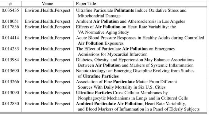
3.2 Top 10 High Impact Papers in Topic “Air Pollution” (Topic 175, PMC) . . . 30

3.3 Dominant 10 Topics in AAN (100 topics) . . . 33

3.4 Dominant 10 Topics in PMC (500 topics) . . . 33

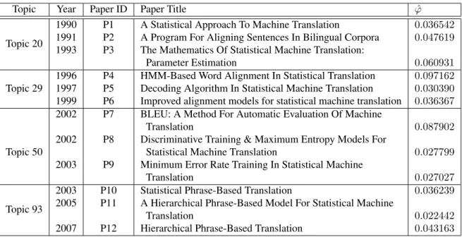
3.5 SMT Example for Theme Evolution . . . 37

3.6 Loss on Forward Citation (AAN) . . . 38

3.7 Loss on Journal Conditional Entropy (PMC) . . . 39

4.1 Summary of Notations . . . 45

4.2 Crowd Pairwise Preferences Binding Performance (Kendall’s tau Distance) . . . 54

4.3 TPPPerformance with More Workers but Sparser Annotation (Kendall’s tau Distance) . . . 57

5.1 Log-Likelihood on Semantic-Syntactic Word Relationship Dataset . . . 74

6.1 Phrasal Allocation Evaluation . . . 85

6.2 Top phrases in tCRP . . . 86

6.3 Nearest Neighbors of Phrases. . . 87

(10)

List of Figures

1.1 Pearson’s Mixture of Two Normals on “Breadth of Forehead of Crabs” . . . 3

1.2 Comparison of the mixture model of two normals between Pearson’s approach and EM algorithm. The two mixture models are very close to each other showing that the moment-matching method of Pearson obtains a near optimal likelihood.. . . 5

2.1 A illustration of the relationship betweenf and its conjugatef∗. For a givens∗, since f(x) ≥ hs∗, xi −f∗(s∗)always holds, which means that in the plot the curve off(x)is always above (or on) the line ofhs∗, xi −f∗(s∗). As a limiting case,< s∗, x∗ >−f∗(s∗)is cuttingf(x)atx=x∗. In addition, the affine function intersects the vertical axisx= 0at the altitude−f∗(s∗). The plot also shows the relationship betweens∗andx∗can be described by thegradient mapping:x∗ ∈∂f−1(s∗), or equivalentlys∗∈∂f(x∗). . . 13

3.1 An illustration of the proposed evolution graph. We show 5 topics, and their dependency. Topic 2 and 3 are enabled by Topic 1 while Topic 5 is enabled by Topic 3 and 4. . . 20

3.2 Topic Temporal Strength for “WSD” and “DP” . . . 32

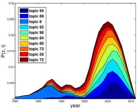
3.3 Topic-Temporal Joint Strength In AAN . . . 35

3.4 Topic-Temporal Joint Strength In PMC. . . 35

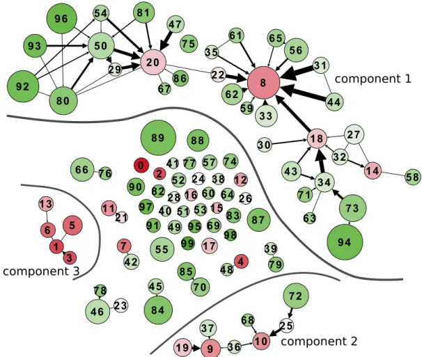
3.5 Theme Evolution Graph of AAN . . . 36

3.6 Temporal Evolution in Topics of Theme SMT . . . 38

4.1 Plate notation for TRM . . . 44

4.2 Plate notation for TPP. . . 44

4.3 An Illustration Example of TPP: The generation of two pairwise preferences by a crowd worker for a given query . . . 47

4.4 Domain Prediction Accuracy and Model Log Likelihood with Standard Deviations . . . 56

4.5 NDCG@n evaluated on MQ2008-agg Dataset . . . 57

4.6 R.O.C. Curve for Malicious Worker Detection . . . 58

5.1 Dual Clustering in the Simplex with KL-divergence . . . 71

5.2 Performance on Text Classification and Word Embedding . . . 73 6.1 Curves of average customers per table, number of tables, the number of days when tables are pruned,

(11)

Chapter 1

Introduction

The general treatment of data mining and machine learning problems can be categorized into two classes: probabilistic methods and non-probabilistic methods. For classification applications, for example, probabilistic methods include logistic regression, maximum entropy, and conditional random fields, for binary, multi-class, and sequential predictions, respectively. The non-probabilistic counterpart includes the well known support vector machines (or the more general max-margin methods), which is also investigated for binary, multi-class and structure predictions. In clustering problems, one of the most widely used probabilistic methods is the family of mixture models while matrix factorizations are usually adopted in non-probabilistic settings. The focus of this thesis is on the probabilistic methods, which have several important advantages: (1) Probabilistic models assign probabilities instead of real-value scores to outcomes (cluster id, class label), which convey statistical uncertainty. Also, the measurement of probability is intuitive and statistically meaningful. (2) In contrast to the optimization within the non-probabilistic framework, where expert knowledge is required to determine the form objective function, probabilistic methods naturally yield a principled and generic optimization paradigm: Maximum likelihood estimation (MLE), or equivalently, Kullback-Leibler (KL) divergence minimization. (3) In Bayesian settings, model regularization can be further achieved by specifying a prior distribution of the model parameters. The optimization problem is then solved by either Maximum A Posterior (MAP) or posterior expectation, which extends MLE. These advantages are appealing both theoretically and practically, which motivates the studies in this thesis.

Probabilistic latent variable models (PLVMs) have provided a mathematical-based approach to the statistical modeling of a wide variety of random phenomena which cannot be explained well by simple distributions, such as binomial, multinomial, Poisson for discrete distributions, and Gaussian, Dirichlet for continuous distributions, respectively. PLVMs assume that the observed data are accompanied by a group of “unobserved” latent variables. And the distribution of the observed data is conditioned on the latent variables. PLVMs are able to model complex distributions through an appropriate choice of the latent variables to represent accurately the local areas of support of the true distribution. Computation can therefore be made feasible through incorporating the latent variables, as the latent variables are usually chosen with a tractable form.

(12)

is mathematically represented by a multinomial distribution over words in a vocabulary. The unigram distribution of a document is then regarded as a “mixture” of the topics. Though the observation is merely words in the documents, by introducing latent variables, namely the topic assignments of words, the semantic relationship of words can be identified to a great extent, and the prominent subject of a document can be revealed as well. For instance, in topic modeling such as Probabilistic Latent Semantic Indexing (PLSI) and Latent Dirichlet Allocation (LDA), words like “science” and “technology” would both have a large probability in a particular topic of scientific research, while “baseball” and “basketball” would both have a large probability in another topic of sports. In computer vision, topic modeling is also

applied to the task of image segmentation where pixels of an image are seen as a mixture of latent objects.

We devote the rest of this section to illustrate how we can leverage probabilistic latent variable models for knowledge discovery and optimization.

1.1 Latent Variable for Knowledge Discovery

PLVMs as an extremely flexible method of modeling have been extensively studied for knowledge discovery. In recent decades, from probabilistic latent semantic indexing, latent Dirichlet allocation, to Dirichlet process, Indian buffet process, literatures have witnessed numerous PLVMs being proposed and widely applied to varying fields such as natural language processing, speech recognition, and computer vision. In this section, we restrict our analysis to mixture models, also better known as topic modeling in recent literature.

1.1.1 Mixture Models — A Historical Account

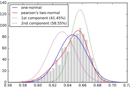
The early research efforts on mixture models can be dated back to1896when Karl Pearson fitted a mixture of two normal probability density functions (Pearson, 1896) on the problem ofBreadth of “Forehead” of Crabs. As a pioneering biostatistician, he has been credited for the finite mixture models and method of moments among his other contributions. In hindsight, his work also established the computational (optimization) theory of statistical modeling, a difficult yet interesting research area even today, which inspires my study on this topic composing most of this thesis. The dataset on which Pearson modeled consisted of measurement on the ratio of forehead width to the body length of 1000 crabs sampled at the Bay of Naples by zoologist W.F.R. Weldon. Weldon analyzed the histogram of the observations, which is plotted in Figure1.1a, along with a normal distribution fitted using Maximum Likelihood (see the solid blue line). However,Weldon(1893) speculated that the asymmetry in the histogram, “a well-marked deviation from this normal shape,” could be resulted from a hypothesis that “the units grouped together in the measured material are not really homogeneous.” To validate whether the population of crabs was evolving toward two subspecies, he turned to his colleague Pearson for help on mathematics.

(13)

0.56 0.58 0.60 0.62 0.64 0.66 0.68 0.70 0.72

0

20

40

60

80

100

120

140 one-normal

pearson's two-normal

1st component (41.45%)

2nd component (58.55%)

(a) In this plot, the bar chart of the observations from Weldon is shown in grey. The blue solid line shows the single normal distribution fitting the data using Maximum Likelihood; And the solid line in red plots the mixture model of two normals distributions derived by Pearson using moment matching where its two components are also displayed in green and purple dotted lines.

0.56 0.58 0.60 0.62 0.64 0.66 0.68 0.70 0.72

0

20

40

60

80

100 pearson's two-normal

Weibull

(b) Comparison between the Pearson’s mixture of two normals and a single Weibull distribution. Pearson’s mixture model provides a tighter fitting at the mode of empirical distribution. Note that the density function of Weibull distribution is much more complicated than that of normal distribution and it requires numeric means to estimate the parameters.

Figure 1.1: Pearson’s Mixture of Two Normals on “Breadth of Forehead of Crabs”

Pearson used two normal distributions to fit the observations. He assumed that the observed data are sampled fromπ1N(µ1, σ21) +π2N(µ2, σ22), (π1+π2 = 1). To estimate the parameters, namely, the means (µ1, µ2) and

(14)

standard-variance (σ1, σ2) of the two normal distributions as well as the proportions (π1, π2) of the two components,

Pearson followed the method of moments (which was also introduced by himself in 1894). Though moment matching is superseded by Fisher’s method of maximum likelihood (Pfanzagl,1994) in nowadays classic statistical modelling, it was a relatively numerically simpler approach in most cases. However, the calculation was still formidable and daunting at the time without the aid of computer or other machinery of any kind. Mathematically, the problem involves five parametersµ1, µ2, σ1, σ2andπ1(since we can obtainπ2= 1−π1) and to find a solution, the parameters need to

ensure that the mixture model matches on the first five moments. Pearson derived a ninth degree polynomial (nonic) and two candidate real roots are found. He finally chose the solution on the basis of agreement with the sixth moment. In Figure1.1a, the dashed curve in red shows Pearson’s mixture and its two components are displayed in purple and green dotted lines. Clearly, the mixture is skewed and better fits the histogram than a single normal distribution. And indeed, two subspecies are identified which verifies the hypothesis of Weldon.

It is quite an advanced idea to leverage latent variables for statistical modeling at that time. Otherwise properly fitting the asymmetric observations would involve a much more complicated distribution. In fact, we can also explain the data with a skewed Weibull distribution, the parameter of which are nevertheless computationally difficult to estimate (The Maximum Likelihood estimator for the shape parameter is the solution to the equation_k1 =PNi=1(x

k ilogxi−xkNlogxN) PN i=1(xki−xkN) − 1 N N P i=1

logxi, and numeric methods, which were very primitive at the time of late 19th century, is required). Therefore Weibull distribution was not a practical option for Pearson to fit the data when the aid of computers was not available. In Figure1.1b, we compare Peason’s mixture of two normals with one single Weibull distribution fitting the data using Maximum Likelihood. The difference between the two curves is not significant. However, Pearson’s result seems to fit better at the mode around0.66.

1.1.2 Mixture Models — Development of the EM Algorithm

Although solving the mixture model with the method of moments is a very laborious task and performing the necessary calculation is even more heroic (McLachlan and Peel,2004), it does not always yield the optimal solution in the statistical sense. The maximum likelihood approach, however, possesses superior statistical property as it tries to place higher probability close to the observed data and are more often unbiased. With the development of optimization in the modern computer science, statistical modeling is able to utilize numerical algorithms to solve Maximum Likelihood Estimation (MLE). Among the different optimization methods, the Expectation-Maximization (EM) algorithm (Dempster et al., 1977) has greatly stimulated interest in the use of mixture models as well as other PLVMs. Several reasons can be accounted for the popularisation of the EM algorithm: (1) It is generally easy to implement the algorithm and it has virtually no parameters to tune, as compared to, for example, gradient descent, where a carefully selected learning step

(15)

model. For example, in the normal mixture problem, the standard-variance of a component normal is always positive. In the EM algorithm, this is naturally satisfied since it is computed as the empirical standard-variance of the complete data generated out of the posterior distribution; (3) EM is a flexible family of approaches where the variational distribution in the expectation step can be simplified (or constrained) for the purpose of computation efficiency (e.g. mean-field EM and convex relaxations, (seeWainwright and Jordan,2008, Chapter 5, 7)) and the maximization step can also be substituted by an ascend step. We leave the details of EM algorithm in Section2.2. In this section, we provide a brief comparison between EM algorithm and Pearson’s method of moments and show how Pearson’s result can be improved by the EM algorithm.

0.56 0.58 0.60 0.62 0.64 0.66 0.68 0.70 0.72

0

20

40

60

80

100

120

140 pearson's two-normal

EM's two-normal

Pearson's 1st comp. (41.45%)

EM's 1st comp. (44.32%)

Pearson's 2nd comp. (58.55%)

EM's 2nd comp. (55.68%)

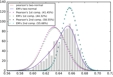
Figure 1.2: Comparison of the mixture model of two normals between Pearson’s approach and EM algorithm. The two mixture models are very close to each other showing that the moment-matching method of Pearson obtains a near optimal likelihood.

We plot the curves of the mixture models of the two methods as well as their components in Figure1.2. The results are almost identical. To assess the quality of the model quantitatively, Pearson used the Chi-square test (Pearson,1900) which he proposed to examine if the observed data is indeed from the model. We follow his practice and report the result in Table1.1.

As expected, we see that the EM algorithm results in the smallest Pearson’s Chi-square. In less mathematical terms, the observed data is distributed more close to the model given by the EM algorithm. In addition, the p-values in the significant test show that it is more certain that the data is sampled from the mixture normal of EM algorithm. To an extent, the assessment on the Weldon’s crab dataset justifies the use of EM algorithm to solve MLE in applications of

(16)

Table 1.1: Pearson’s Chi-square test and p-Value for a single normal model, a single Weibull model, and the two normal mixture model of Pearson and EM algorithm in the “Breadth of Forehead of Crabs” problem. For the normal models, we also include the model parameters.

Method µ1 µ2 σ1 σ2 π1 π2 freedom Chi-square p value

Single Normal 0.6466 — 0.0190 — 1 — 2 71.6836 2.157×10−6

Single Weibull — — — — — — 2 28.3841 0.2904

Pearson 0.6326 0.6566 0.0179 0.0125 0.4145 0.5855 5 21.0342 0.5186

EM 0.6339 0.6568 0.0182 0.0124 0.4432 0.5568 5 20.8438 0.5304

mixture modeling.

1.1.3 From Mixture Models to Topic Modeling

Since late 1990s, the study on document understanding has witnessed a new approach of PLVMs which is often referred to as topic modeling. The first well recognized topic modeling method, probabilistic latent semantic indexing (PLSI) (Hofmann,1999), is simple yet effective. Essentially it sees the unigram word (wd) distribution of a documentdas aK-mixture of multinomial distributionsβ1, . . . , βKwith proportionsθd,1, . . . , θd,k. ThoseβKare referred to as “topics” because the words of large probabilities in a component are often semantically related. In addition, the topic weightsθdof a document provides a succinct summary of the documents. Computationally,θd has a much lower dimensionality thanwd and thus can be leveraged as a (part of) feature vector in tasks such as document classification or clustering. Moreover,θd is semantically meaningful as the similarity ofθd’s correlates with the similarity of the subject of documents, which can be greatly useful in document understanding, information indexing, etc.

In terms of modeling the latent variables, there are two milestone progresses: the Bayesian inference and nonparametric statistics. The early efforts promoting the Bayesian nonparametrics and advocating the theoretical formalization of topic modeling, specifically, the analysis on random processes of exchangeable partitions (Pitman, 1995), are the lectures taught byPitman et al.at Berkeley in Spring2002. Many results obtained in this direction (Blei and Lafferty,2009;Blei et al.,2003,2010) are immediate fruit of the course and readers interested in a principle introduction on this topic should refer to the lecture notes (Pitman et al.,2002) and the references therein.

Bayesian inferencedeparts from the traditional MLE framework. It assumes a prior distribution on latent variables parametrized by thehyperparameters. The advantages of introducing a prior on latent variables are mainly two folds and we show them using the Latent Dirichlet Allocation (LDA) (Blei et al.,2003) as an example: (1) It enables user to incorporate human knowledge about the latent variables into modeling. In document understanding, the word distribution of a topic as well as the proportion of topics for a document are naturallysparse. LDA encourages such behavior by using a Dirichlet prior with a small hyperparameterα. (2) By selecting the form of prior distribution

(17)

conjugate prior-posterior pairs are computationally beneficial in both Gibbs sampling as well as variational inference. LDA chooses Dirichlet as the conjugate prior to the multinomial distribution, and the posterior distribution is also a Dirichlet of parameterα+n, wherenis often referred as the pseudo-count of the latent variables in each topic. Estimation method for Bayesian inference has also been greatly developed beyond MLE. There are two major estimation methods of the latent variables in Bayesian setting which are Bayesian Estimator (Posterior Expectation) and Maximum a Posterior (MAP). The first computes the posterior expectation of the latent variables given the observed data while the second selects the value with the maximal probability in the posterior distribution, which can be viewed as an extension of the MLE method. In the context of topic modeling, it has been noticed that Bayesian estimator is more popular than MAP. The major criticism of MAP is the fact that it is still a point estimation in nature. Specifically in topic modeling, it is not uncommon that the posterior distribution of the latent variables are in fact multi-modal. And therefore it is computationally infeasible (or even intractable) to calculate MAP due to the non-convex nature of the problem.

Nonparametric statisticsaims to model the data with possibly infinite number of latent variables. In topic modeling, it implies that one can model a infinite number of topics or words in the vocabulary. Although in practice it does not seem to be immediately useful since there is always a finite upper-bound for these quantities, it is critical to rely on expert knowledge to appropriately select the values. Nonparametric statistics are most powerful to adaptively learn the number of latent variables that are adequately large to explain the data by using random processes. Random processes are extensively studied in recent literature, as surveyed in (Hajek,2015), including Gaussian process (Rasmussen and Williams,2006), Dirichlet process (Teh,2011), Indian buffet process (Ghahramani and Griffiths,2005), and hierarchical processes (Blei et al.,2010;Griffiths and Tenenbaum,2004;Teh et al.,2012), just to name a few. Mathematically, to model the latent variables from possibly infinite number of choices, the nonparametric approach assumes a random process as prior. Computationally, there are mainly two strategies, Gibbs sampling and truncated variational inference, to estimate the posterior distribution of the possibly infinite number of latent variables. Gibbs sampling takes advantage of the fact that the prior process usually yields a simple prediction rule of one latent variable given all others. For example, in Dirichlet process, using the notion of Chinese restaurant process (Pitman et al.,2002), the probability of a latent variable choosing an existing value is proportional to the number of other latent variables of the same value, or a new value proportional to the hyperparameterα:

PCRP(zi=k|z1, . . . , zi−1, zi+1, . . . , zN)∝        N P j=1,j6=i 1(zj=k) ifk < K α ifk=K+ 1 (1.1)

(18)

Therefore it is feasible to investigate sampling methods for inference. While alternatively, another strategy for estimation is to approximate the possibly infinite posterior with a finite approximation. For the Dirichlet Process (as well as the generalized Pitman-Yor two-parameter process (Pitman and Yor,1997)), the truncating approximation is based on a stick-breaking (Ishwaran and James,2011) interpretation. It views the process as breaking a stick with the proportion as a sample from a Beta distribution and the truncation stops the breaking after there is a predefined number of sticks generated. Both of the above two strategies have advantages: Gibbs sampling does not need to truncate the size of latent variables by a finite number, while the truncated variational inference is generally computational efficient. However, as shown in (Wang and Blei,2012), it is possible to combine the two ideas together by performing the E-step in variational EM via sampling.

1.2 Latent Variables for Optimization

Previous research such as topic modeling mainly incorporates the latent variables for the purpose of knowledge discovery. Another motivation to use latent variable models is efficient computation. In previous discussion of the “Breadth of Forehead of Crabs” example, we have already seen that by introducing latent variables, the mixture model is much easier to compute than that of the Weibull distribution. However, contemporary efforts in the direction of leveraging PLVMs for efficient computation was less explored. In one of our recent work, Dual-Clustering Maximum Entropy (DCME) (Wang et al.,2016b), it is demonstrated that PLVM is an effective means to improve the optimization efficiency.

We explore PLVM in the context of Maximum Entropy (ME) models. ME is a classic approach in classification as well as word embedding. However, it becomes computationally challenging when the number of classes or the vocabulary size is large. DCME approaches the problem by optimizing ME in its primal-dual form. The key insight is to introduce a latent cluster assignment for each training instance and assume that the dual variables of an instance are determined by the corresponding latent assignment. As an initial investigation, we use the latent variables in a much simpler manner than the mixture models. Specifically, we restrict the latent variable to distribute as a Kronecker delta which has support only on a single value, in contrast to the case of mixture models where the latent variable is subject to a more general multinomial distribution. DCME naturally leads to an approximation of the dual variables which can be computed by a K-means like clustering. More importantly, it enables an efficient online-offline computation scheme whose computational complexity does not depends on the number of classes nor the vocabulary size. Empirical studies demonstrated that DCME significantly outperforms state-of-the-art approaches.

(19)

1.3 Contribution of this Thesis

In this thesis, I describe a range of applications where latent variables can be leveraged for knowledge discovery and efficient optimization. Works in this thesis demonstrate that PLVMs are a powerful tool for modelling incomplete observations. Through incorporating latent variables and assuming that the observations such as literature citations, pairwise preferences in crowdsourcing as well as unstructured text are generated following tractable distributions parametrized by the latent variables, PLVMs are flexible and effective to discover knowledge in data mining problems, where the knowledge is mathematically modelled as continuous or discrete values, distributions or uncertainty. For example, when modelling literature citations, latent variables can be inferred to identify research topics and evolution of research themes; While only observing pairwise preferences labelled by non-expert workers in crowdsourcing, PLVM as a generative process is capable to recover the ground truth ranked lists; And finally, by fitting the unstructured text with underlying phrasal structures, it can be shown that both the phrasal allocation and phrase embeddings are effectively computed. In addition, I also explore the PLVMs for deriving efficient algorithms. It has been shown that latent variables can be employed as a means for model reduction or to facilitating computation/sampling of intractable distributions. For instance, PLVM has been shown to improve efficiency of Maximum Entropy which does not scale well as the number of classes by performing model reduction with the latent variables; In addition, in cases where the computation involves a intractable distribution, latent variables are also investigated to facilitate the calculation via Gibbs sampling.

1.4 Overview of this Thesis

In Chapter2, we briefly discuss a few key mathematical ingredients that can greatly facilitate the understanding of PLVMs. Next, we move on to show two scenarios where PLVMs are applied for knowledge discovery in Chapter3 and Chapter4. Leveraging PLVMs for efficient optimization is presented in Chapter5. The last work we propose in this thesis takes the advantages of PLVMs in both aspects, namely extracting the phrasal structure with an efficient optimization scheme and effectively learning the semantic embeddings of phrases, is discussed in Chapter6.

The first work analyzes the citations of literatures (Wang et al.,2013). Understanding how research themes evolve over time in a research community is useful in many ways (e.g., revealing important milestones and discovering emerging major research trends). In this study, we propose a novel way of analyzing literature citation to explore the research topics and the theme evolution by modeling article citation relations with a probabilistic generative model. The key idea is to represent a research paper by a “bag of citations” and model such a “citation document” with a probabilistic topic model. We explore the extension of a particular topic model, i.e., Latent Dirichlet Allocation (LDA), for citation analysis, and show that such a Citation-LDA can facilitate discovering of individual research topics as

(20)

well as the theme evolution from multiple related topics, both of which in turn lead to the construction of evolution graphs for characterizing research themes. We test the proposed citation-LDA on two datasets: the ACL Anthology Network (AAN) of natural language research literatures and PubMed Central (PMC) archive of biomedical and life sciences literatures, and demonstrate that Citation-LDA can effectively discover the evolution of research themes, with better formed topics than (conventional) Content-LDA.

The second work explores PLVMs in a crowdsourcing setting (Wang et al.,2016a). Crowdsourcing services make it possible to collect huge amount of annotations from less trained crowd workers in an inexpensive and efficient manner. However, unlike making binary or pairwise judgements, labeling complex structures such as ranked lists by crowd workers is subject to large variance and low efficiency, mainly due to the huge labeling space and the annotators’ non-expert nature. Yet ranked lists offer the most informative knowledge for training and testing in various data mining and information retrieval tasks such aslearning to rank. In this paper, we propose a novel generative model called “Thurstonian Pairwise Preference” (TPP) to infer the true ranked list out of a collection of crowdsourced pairwise annotations. The key challenges that TPPaddresses are to resolve the inevitable incompleteness and inconsistency of judgements, as well as to model variable query difficulty and different labeling quality resulting from workers’ domain expertise and truthfulness. Experimental results on both synthetic and real-world datasets demonstrate that TPPcan effectively bind pairwise preferences of the crowd into rankings and substantially outperforms previously published methods.

Another aspect of PLVMs is to improve the efficiency of optimization. To this end, we devote another chapter to discuss the study of Dual-Clustering Maximum Entropy (Wang et al.,2016b). Maximum Entropy (ME), as a general-purpose machine learning model, has been successfully applied to various fields such as text mining and natural language processing. It has been used as a classification technique and recently also applied to learn word embedding. ME establishes a distribution of the exponential form over items (classes/words). When training such a model, learning efficiency is guaranteed bygloballyupdating the entire set of model parameters associated withallitems ateach training instance. This creates a significant computational challenge when the number of items is large. To achieve learning efficiency with affordable computational cost, we propose an approach named Dual-Clustering Maximum Entropy (DCME). Exploiting the primal-dual form of ME, it conducts clustering in the dual space and approximates each dual distribution by the corresponding cluster center. This naturally enables a hybrid online-offline optimization algorithm whose time complexity per instance only scales as the product of the feature/word vector dimensionality and the cluster number. Experimental studies on text classification and word embedding learning demonstrate that DCME effectively strikes a balance between training speed and model quality, substantially outperforming state-of-the-art methods.

(21)

methods are intrinsically hindered by its unigram (bag-of-words) assumption of language. Although efforts towards resolving the semantics for higher level of language units (e.g.phrase, sentence) have been made, most of them either rely on an external resource or employ a complicated decoding algorithm for identifying the composition structure. In this work, we propose an effective yet simple generic algorithm, Phrasal Latent Allocation with Negative Sampling (PLANS), to compute the phrase embedding. We propose transient Chinese Restaurant Process (tCRP) as a prior for words to allocate the phrases within which they are enclosed. In addition, similar to Skipgram, PLANS estimates the embedding for words/phrases with negative sampling. Nevertheless the major challenge in learning is that a reasonable size of the phrases need to be carefully retained and less confident ones are constantly pruned during training. PLANS address this with an online block algorithm which refreshes the set of phrases based on their “frequencies” in the corpus periodically. In addition, simulated annealing (SA) is applied in the sampling process to

(22)

Chapter 2

Background

For self-containedness, we provide a short reference to the mathematical tools that we have been frequently used in PLVMs. Readers familiar with the theory of conjugate duality and EM algorithm can skip the content of this chapter. And for a comprehensive account, please refer to the book (Hiriart-Urruty and Lemarechal,1993).

2.1 Conjugate Duality

The conjugate in optimization context refers to the transformation of a problem to another accompanying problem. The transformation is also known as theconjugacyoperation or theLegendre-Fencheltransformation. It plays an important role in the Lagrangian duality as well as the general convex optimization. To start our discussion, we formally define the conjugate of a function as:

Definition 2.1.1. The conjugate of a convex function1f is the functionf∗defined by

f∗(s) = sup{hs, xi −f(x)}, ∀x∈domf (2.1) An geometrical interpretation of the conjugate of a subdifferentiable function is illustrated in Figure 2.1. A immediate result is that:

Theorem 2.1.1. For anyx∗∈arg max{hs∗, xi −f∗(s∗)}, we have thatx∗∈∂f−1(s∗)

In addition, the conjugacy transformation is generally symmetric:f∗∗=f for convex functions. To be exact, the identity between the bi-conjugatef∗∗_and_f _{is equivalent to the requirement that the convex}_f _{is lower semi-continuity}

(l.s.c):lim inf x→x0

≥f(x0), a sufficient condition of which is thatfis subdifferentiable.

Log-Partition and Negative Entropy

One important instance of the conjugate in PLVMs is between log-partition and negative entropy, which are defined as: 1_{we make a stronger assumption that}_f_{is convex which can relaxed to the existence of a affine function memorizing}_f_on_dom_f_.

(23)

−2 0 2 4 −2 −1 0 1 2 3 4 5 6

(0, − f

∗

_(s

∗

₎₎

(x

∗

_{, f(x}

∗

₎₎

f(x) s∗_{, x − f}∗_(s∗₎

Figure 2.1: A illustration of the relationship betweenf and its conjugatef∗. For a givens∗, sincef(x)≥ hs∗, xi −

f∗(s∗)always holds, which means that in the plot the curve off(x)is always above (or on) the line ofhs∗, xi −f∗(s∗). As a limiting case,< s∗, x∗>−f∗(s∗)is cuttingf(x)atx=x∗. In addition, the affine function intersects the vertical axisx= 0at the altitude−f∗(s∗). The plot also shows the relationship betweens∗andx∗can be described by the gradient mapping:x∗∈∂f−1₍_s∗_{), or equivalently}_s∗_∈_∂f₍_x∗_).

Log-Parition: A(x) = log N X i=1 exp(xi) (2.2) Negative Entropy: −H(p) = N X i=1 pilogpi (2.3)

wherepis an element in the simplex set which is defined as:

∆N ={p∈RN :pj ≥0, N

X

j=1

pj = 1}

The log-partition function is often seen in Maximum Entropy models, energy-based models, as well as Markov Random Fields, etc. The straight-forward computation involves a summation overNitems, which can be computationally challenging ifN is large. For example, in Markov Random Fields,N =m!wheremis the number of nodes in the random fields. Computing the log-partition function is often the bottleneck for training such a model.

(24)

Lemma 2.1.1.1. Assume that P(i;s) = exp(si) N P j=1 exp(sj) and A(s) = log N X j=1 exp(sj)

The conjugate duality between the log-partition function and negative entropy states:

A(s) = max µ∈∆N { N X j=1 µjsj− N X j=1 µjlogµj} = max µ∈∆N {Eµ[sj] +H(µ)} (2.4)

where the maximizer is attained at:

µ∗_j = P(j;s), 1≤j≤N (2.5)

Proof. In light of Theorem2.1.1, the general proof of the conjugacy transformation betweenfandf∗is to verify that

x=∂f∗ ∂f(x)

. And it is easy to show that

s=−∂H ∂A(s)

However, it is much more intuitive to alternatively prove by showing the equivalence in Equation (2.4). We follow the derivation: Eµ[sj] +H(µ) =− N X j=1 µjlog µj P(j;s)+ log N X j=1 exp(sj) =−DKL(µ||P) +A(s)

whereDKL(µ||P)is the Kullback-Leibler (KL) divergence. Note that KL-divergence is always nonnegative:

DKL(µ||P)≥0 and:

(25)

DKL(µ||P) = 0 ⇐⇒ µ=P It follows that:

µ∗= arg min µ∈∆N

DKL(µ||P) =P

2.2 EM Algorithm: a Modern Reinterpretation

Equipped with the conjugate duality, here we offer a new interpretation of the famous EM algorithm. Part of the idea presented here is also shared by the work (Iusem and Teboulle,1992).

Suppose that there is a distributionP(Z|Θ)where the dataZ= (X, Y)is partially observed and can be decomposed into the observationsXand the unseen variablesY. Given a set of dataX1, . . . , XN, MLE solves the problem:

max

Θ log P(X1, . . . , XN|Θ)

Using the conjugate duality proved in Theorem2.1.1:

log P(X1, . . . , XN; Θ) = N X i=1 logX Yi P(Xi, Yi; Θ) = N X i=1 max µi∈∆ X Yi µi,Yilog P(Xi, Yi; Θ) +H(µi) (2.6)

Therefore, the MLE with incomplete observation amounts to:

max Θ µi∈∆,1≤i≤N N X i=1 X Yi µi,Yilog P(Xi, Yi; Θ) +H(µi) | {z } F(Θ,M)

And for fixedΘ, the optimality condition forµiis:

E-step: ∂F

∂µi

(26)

which is exactly the E-step in EM algorithm. In addition, to optimizeΘwhile fixingM:

M-step: max Θ N X i=1 X Yi µi,Yilog P(Xi, Yi; Θ) (2.8) In the EM algorithm, N P i=1 P Yi

µi,Yilog P(Xi, Yi; Θ)is referred asevidence lower bound(ELBO) function, and the

above maximization is identical to the M-step in the EM algorithm.

Using this interpretation, it is also straight-forward to view the EM algorithm as a coordinate-descent algorithm where the objective function is constructed asF(Θ, M), which is always a lower bound of the log-likelihood. In below, we briefly discuss two important variants of the EM algorithm.

Variant 1: Relaxation by Approximation

In the above basic version of EM, we assume thatµican freely choose any element from the simplex∆. Nevertheless, it often posits a computational difficulty when solving the posterior distributionP(·|Xi; Θ). And it makes sense to trade accuracy ofµifor computational efficiency, and to compute an approximation ofµiby a tractable surrogate, which motivates us to study different approximation approaches in the variational inference. In below, we discuss a few well adopted methods.

Mean-Field Approximation: The simplest strategy for approximation is to restrictµito be chosen from a subset, say, Sinstead of∆. Then the optimization problem forµiwith a constantΘbecomes:

min µi∈S

DKL µi||P(·|Xi; Θ)

(2.9) WhenP(·|Xi; Θ)∈ S, Equation (2.6) will not hold. In such cases, the solution of/ Θwill neither converge to that of MLE. Moreover, because of the restrictedµi∈ S(∆, the EM algorithm with mean-field approximation is in fact

maximizing a (strict) lower bound of the log-likelihood objective.

Approximation by Sampling: As discussed above, it is not uncommon that the posteriorP(·|X,Θ)does not yield a feasible solution. However instead of compute the density analytically, it is generally possible to use a Gibbs sampler to efficiently sample from the distribution. And when incorporating such sampling-based E-step into the EM framework, it is advantageous to run the Gibb sampler for only a few iterations (before its converging) to collect the statistics for maximization in M-step (Wang et al.,2016a), the idea of which can be justified similarly as that of Contrastive Divergence (Carreira-Perpinan and Hinton,2005).

(27)

General Density Approximation: General methods for approximation ofP(·|X,Θ)digress from the optimization framework of EM algorithm by substituting the objective of Equation (2.9) with other forms of measurement for closeness. For example, Belief propagation (Yedidia et al.,2005), Bethe approximation (Burgess and Tully,1978) as well as expectation propagation (Minka,2001a), when used in EM do not yields a lower bound nor upper bound of the log likelihood. Nevertheless, they are extensively investigated for their empirical improvement in terms of efficiency and performance. Especially, the expectation propagation (EP) method was applied to replace the E-step in the EM framework and it outperforms the mean-field alternatives in cases when evidence is limited (Wang and Blei,2012). The EP method can be viewed as an approximation to the minimization of the reversed KL-divergence (Minka et al.,2005):

min µi∈S

DKL P(·|Xi; Θ)||µi

(2.10) Comparing Equation (2.10) to Equation (2.9), we see that the order of two distributions in the KL-divergence is reversed. The in-depth discussion of this topic is beyond the scope of this thesis, and we refer the readers to the brochure on variational inference (Wainwright and Jordan,2008) and the Ph.D thesis ofMinka(2001b) on approximation in Bayesian inference for a complementary review.

Variant 2: Bayesian Variational Inference

EM algorithm is also investigated in Bayesian setting although most techniques remain the same. Specifically,Θis viewed as a distribution which is governed by hyperparameterΓ, and thus the log-likelihood function involves not only marginalizing the latent variableY but also the parameterΘ.

In the Bayesian setting, EM is more often called as Bayesian variational inference method. Mathematically,Θis also a latent variable, no different fromY, and we can still employ the EM algorithm. However, with sufficient observations, the optimization of hyperparmeterΓis less interested and the M-step is generally skipped. More importantly, by carefully choosing the form of the prior distributionP(Θ; Γ)(as conjugate prior ofP(Y; Θ)), we have the posterior P(Θ|Y; Γ)in the same family of distributions as the prior. This is appealing since the update ofµiin Equation (2.6) can be maximized exactly easily.

2.3 Minimax Theory

In this section we will review some results in the minimax theory which gives the conditions under which the following equality is hold:

max

(28)

von Neumannis credited with the first investigation of this problem. There are many different sufficient conditions that guarantees the above equation. Modern analysis employs Farkas Lemma in the min common/max crossing framework and an excellent formal discussion can be found in (Bertsekas et al.,2003). In this thesis, we only present an earlier version of minimax theory by Sion (Sion et al.,1958), which is one of several celebrated generalizations of von Neumann’s minimax theorem (von Neumann,1928):

Theorem 2.3.1(Sion’s Minimax Theorem). LetXandZboth be a compact convex set. Letφbe a real-valued function onX×Z such that:

1. φ(x,·)is upper semi-continuous and quasi-concave onY for anyx∈X

2. φ(·, y)is lower semi-continuous and quasi-convex onXfor anyy∈Y

Then,

max

z∈Z minx∈Xφ(x, z) = minx∈Xmaxz∈Z φ(x, z)

An elementary proof of Sion’s minimax theorem can be found in (Komiya,1988). The derivation is simple, short and elegant. Also, the assumption made in theorem2.3.1is often satisfied for most practical problems under mild assumptions ofφ. In general, Equation (2.11) holds when solving problems involving the dual formulation in PLVMs.

(29)

Chapter 3

Understanding the Evolution of Research

Themes: a Probabilistic Generative Model

for Citations

3.1 Introduction

In this chapter, I demonstrate that by modeling literature citations as observations of a generative model with latent variables, research topics as well as evolution themes of research can be identified and described inactively. It exemplifies that PLVM is an effective means for knowledge discovery in data mining problems. Though we use literature citation as the test bed for PLVM, the method presented here can be easily applied to any general network data as well.

How to leverage information technologies to improve the productivity of scientific research is a highly important challenge with clearly huge impact on the society. One bottleneck in research productivity is that as a research community grows, it would be increasingly difficult for researchers to see the complete picture of how a field has been evolving, given the fact that large volume new literatures are written based on previous works. Junior researchers can often get lost in the overwhelming amount of related papers. Researchers who seek to shift to a new topic may spend lots of time preparing a reading list on his/her own. All these clearly hinder the progress of scientific research, and it would be highly beneficial to develop mining techniques to help researchers more easily and more efficiently understand research themes in scientific literature. In general, two aspects of analysis are needed for understanding research themes: First, we need to analyzeeach research topicto answer the following questions: Which papers are the milestone papers that best represent a topic and how to quantify their impact? When did the topic become popular and is it still attracting attention today? Can the topic be summarized accurately with a few keywords? Furthermore, wheninvestigating topics collectively, which are the most dominant topics extensively studied? During the evolution, what are the newly generated topics initiated by the old one? Can we identify the underlying evolution patterns among topics?

To answer the questions raised above, ideally, we would like to automatically construct a“research theme evolution graph”, which we illustrate in Figure3.1. With such a graph, when zooming into the scope of individual topics, multiple types of information are provided to facilitate users to understand the research topic:

(30)

Figure 3.1: An illustration of the proposed evolution graph. We show 5 topics, and their dependency. Topic 2 and 3 are enabled by Topic 1 while Topic 5 is enabled by Topic 3 and 4.

of understanding topics. We refer to them as “topic milestone papers”. Milestone papers of a topic provide a good picture how a topic is formed. In Figure3.1, milestone papers are shown in each topic as rectangles and the “size” reflects their importance with respect to topics.

• Topic Temporal Strength: The relative popularity of topics at different times reveals the temporal nature of topics, which can help users to identifycurrentvs.previousresearch topics as well as the rough topic life spans. Intuitively, when many milestone papers occur, the topic draws more attention and becomes popular.

• Topic Keywords: Extracting keywords that can properly summarize a topic would enable users to obtain a brief idea about the topic even without reading its relevant papers, allowing users to fast navigate among topics in search of the most interesting ones.

While zooming out to see the big picture of all related topics in the theme, there is also meaningful information to explore:

• Topic Importance: Quantifying the importance of topics helps a user to discriminate themajorvs.minortopics in a research theme. Topic importance also reflects how well the topic is recognized by the community. • Topic Dependency: Many new topics are built on top of the old ones. Discovering the dependency relation

between topics provides a good guidance for users when searching fororigin/continuingtopics. In Figure3.1, we visualize the dependency strength between topics by the “thickness” of edges.

(31)

• Evolution Patterns: Connecting topics by their dependency illustrates the underlying evolution patterns for research themes. Is there any trend that different topics get merged together to form a new (interdisciplinary) topic, such as Topic 3 and Topic 4 are merged into Topic 5? Or is there a general topic branched into multiple topics that address specialized problems, such as Topic 1 has led to Topic 2 and Topic 3?

To automatically construct such an evolution graph as shown in Figure3.1, the two major computational tasks are: • Discovering the research topics, which includes finding milestone papers, computing the temporal strength, and

extracting keywords for each individual topic.

• Discovering the theme evolution, which includes identifying the topic importance and learning the dependency relation between topics, as well as recognizing the underlying evolution patterns.

Existing approaches, notably those of topic modeling, can generate some (not all) of these components in the evolution graph, but they are far from adequate for the following reasons: First, though there are many works that aim to construct evolution map over time, they rely on pre-segmentation of text streams into fixed time windows, due to either computational issue (Blei and Lafferty,2006;Mei and Zhai,2005;Wang and McCallum,2006) or modeling issue (Wang et al.,2012). Consequently, the topic evolution result would be inevitably sensitive to the choice of temporal granularity of how time is discretized and sliced. Suboptimal granularity of time might result in missing important topics or even lead to inaccurate evolution analysis. Second, the edges in most of the existing evolution graphs, do not reflect thedependency relationbetween topics, and can only reveal thetopic similarityandcorrelation (Blei and Lafferty,2006,2007;Mei and Zhai,2005;Wang et al.,2012). The fundamental limitation is that content-based topic modeling approaches are built onword co-occurrence, which essentially isundirectedunlike the dependency relation. Third, it is difficult for any aforementioned models (including Pairwise Link-LDA (Nallapati et al.,2008)) to assess the impact of documents with respect to different topics, i.e., identifying the milestone papers. Their approaches model topics as distributions over words, and although the text similarity between document and topic can be computed, it would be a substantially different measurement from the documentimpacton a topic.

As hinted above, a major reason why existing topic models are insufficient is that they have not fully exploited citation relations to discover topics. In this chapter, we address these limitations by doing joint analysis of citations and text. Indeed, we will rely more on citation links than on document content, which makes our work different from (Nallapati et al.,2008) and all others. Specifically, we leverage a similar idea to topic modeling and analyze the citation graphs in aprobabilisticmanner. We directly model the generation of citations, which are direct evidence related to“impact”of document as well as“dependency”between topics. Through citation generation, we are enabled to address the core problem of assessing milestone papers based on impact, and estimating the topic dependency. More importantly, our key insight here is that “co-cited papers” are good indicators of research topics, more effective than

(32)

relying on text similarity as in most existing work. Empirical study (Boyd-Graber et al.,2009) has already noticed that it is a subjective yet difficult task to annotate for each word its belonging topic even manually. However, for citations in a published paper written by experienced authors, it would be much easier to determine the topic since most authors make citations prudently and thus citation is muchless noisythan text.

To discover topics based on citations, we propose a novel probabilistic approach to analyze citations by viewing citation graphs as a set of “citation documents” where each is a research paper represented as a“bag of citations”. A paper that citeskother (possibly duplicated) papers would simply be viewed as a“document”withk“tokens”, each corresponding to the ID of a cited paper. With this view, we can model all these citation documents with a generative topic model where we introduce latent topic variables over the citations. This is analogous to the application of a probabilistic topic model to model topics in text documents, but with the important difference that the discovered topics with our model would be characterized by a (multinomial)distribution over research papers, rather than over words as in conventional content-based topic models. In addition, when combined together with additional information, particularly thepublished timeand thetitleof each paper, our model can address the computational tasks of discovering boththe research topicsandthe theme evolution, and constructingthe evolution graphas well.

In the rest of the chapter, we first review some of the related work in Section3.2, which is followed by presenting our probabilistic model for literature citations in Section3.3. After the derivation about one specific model Citation-LDA, we focus our discussion on how to construct the theme evolution graph in Section3.4. Experiment setup and extensive evaluation results will be given in Section3.5. Finally, we conclude our work with future direction in Section3.6.

3.2 Related Work

In recent years, many literature search engines as well as digital libraries have come into use, including Microsoft Academic Search1, Google Scholar2, DBLP3and ACM Digital Library4. They provide knowledge about scientific literatures through ranking and search interface, which in turn, relies on algorithms that utilize citation-related indicators such as H-index (Hirsch,2005) and Impact Factor (Garfield,2006).

In the research community, one thread of study treats scientific literature as citation graphs. To assess the importance of papers, graph ranking algorithms such as PageRank and its variants have been applied (Ghosh et al.,2011;Radev et al.,2009;Sayyadi and Getoor,2009;Walker et al.,2007). In (Ghosh et al.,2011), the authors further take time into consideration in order to overcome the recency bias that favors “old” papers. Apart from this, graph clustering is investigated to identify meaningful topics, such as (Bolelli et al.,2006;Flake et al.,2004;Popescul et al.,2000;

1_{http://academic.research.microsoft.com/} 2_{http://scholar.google.com/}

(33)

Qazvinian and Radev,2008). In (Popescul et al.,2000), it is pointed out that efficient graph clustering can be combined with temporal information to identify the trends of topics in literature. Particularly, one recent paper (Jo et al.,2011) is close to our work. It leverages both citation and text (title and abstract) to generate the evolution map in computer science community. Specifically, their method relies on the temporal order of papers and the document language model to detect the formation of new topics, and then it computes the strength between two topics with the “cross citation count” (total citation numbers between the two topics), which however ignores the directed relation of topic dependency. Their method is difficult to be applied to address our problem because their method does not distinguish the difference in topic importance, nor does it recognize milestone papers through assessing the impact based on citations.

While on the other hand, existing probabilistic topic modeling over text (Blei et al.,2003;Griffiths and Steyvers, 2004;Hofmann,2001) has been throughly studied, treating documents as mixtures of latent topics. Early attempt in modeling the topic evolution (Mei and Zhai,2005) investigates the Probabilistic Latent Semantic Index (PLSI) (Hofmann, 2001) to extract topics and models the evolution process as transitions between topics in Hidden Markov Model (HMM). Later, Topic Over Time (TOT) model (Wang and McCallum,2006) is developed based on Latent Dirichlet Allocation (LDA) (Blei et al.,2003). The key difference between between LDA and TOT is that TOT explicitly assumes time as generated from topics, which jointly models time and word, thus enabling itself to discover time-aware topics as well as topic temporal strength. Besides, Dynamic Topic Models (Blei and Lafferty,2006;Wang et al.,2012) address the problem of topic evolution by modeling topics (distributions over words) changing over time. In the discrete case (Blei and Lafferty,2006), topics at the next time-stamp deviate from the current ones by a Gaussian noise; while, in the continuous case (Wang et al.,2012), the change of topics over time is generalized as Brownian motion. One limitation of these models (Blei and Lafferty,2006;Mei and Zhai,2005;Wang et al.,2012;Wang and McCallum, 2006) is that they all rely on the pre-segmentation of time: without appropriate time granularity selected, they could fall into difficulty in finding important topics. Ideally, the selection of correct time span should be made automatically. In addition to these studies, others consider the problem of modeling topic correlation (Blei and Lafferty,2007) and document hyperlink generation (Chang and Blei,2009), for which the essential difficulty is that they cannot model the“dependency”relation between topics. The only exception we are aware of so far is the paper (Nallapati et al., 2008) which jointly models text and citation generatively. One of its proposed model, named “Pairwise Link-LDA”, explicitly includes the topic dependency as model parameters by extending the idea of mixed-membership block stochastic models (Airoldi et al.,2006). In words, the chance of generating a particular citation is determined by the topics of citing and cited documents, which indeed addresses the topic dependency directly. Nevertheless, the Pairwise Link-LDA is not able to fulfill all the tasks we listed such as recognizing the milestone papers and so on.

To our best knowledge, there is no existing approach that can address all the questions as we raised before, i.e., the discovery ofresearch topicsandtheme evolution. To this end, we directly model the generation of the citation links

(34)

among literatures in this work. In the same spirit of topic modeling, citations are generated stochastically according to a distribution with respect to the underlying topic. It is worth noting that applying the topic modeling approaches to study graphs was previously investigated for discovering communities from coauthorship networks in (Henderson and Eliassi-Rad,2009;Zhang et al.,2007). Nevertheless, our model not only discovers the topics, but also explores their dependency relationships and yields meaningful knowledge about the evolution of topics.

3.3 Probabilistic Modeling of Literature Citations

In contrast to most existing work on citation analysis, where citations are often modeled as network or graph, we propose to represent citation graph as a set of “citation documents” where each is a research paper represented as “bag of citations”, and model these citation documents with a probabilistic generative model. Such a new approach has several advantages over pure graph analysis methods. First, by using a latent topic variable, we can naturally associate topics with papers and citations, enabling ranking the paper based on citation within each topic, through which milestone papers can be identified. Second, by modeling the whole set of papers in a field, we can obtain a set of topics that summarize well the major research topics in the field, with (probabilistic) weights quantifying their importance. Third, by estimating the topic level citation structure, it is possible to compute the strength of dependency relation between topics and picturing the evolution paths of research themes. Last, distribution over papers for each topic obtained by such a model can be easily used to compute a distribution over time or keywords when used together with other information such as paper published time and title, allowing modeling the topic temporal strength and summarizing topics with keywords.

Compared with pure content-based topic models, our use of topic model is entirely on capturing topics through citation structures, roughly corresponding to discovering topics based onco-citation relation, which is intuitively more accurate in finding research topics: if there is a“stable”set of“core papers”that are often cited together, then it generally indicates the existence of a major research topic and the core papers are actuallymilestone papersin that topic. Specifically, we use a probabilistic model to explain how an author generates the references (citations) for a paper (which we may also refer to as a document for convenience sometimes). More specifically, given a paper, he/she would “generate” all the references cited in the paper independently. When generating each citation, the author would first sample a topic according to a document-specific topic distribution (doc topicdistribution), and then draw a reference document to cite from the citation distribution of the sampled topic (topic docdistribution). One may easily notice that such a generation process is essentially similar to the one over words for documents assumed in probabilistic topic models for text data. Indeed, our work is a novel way of using topic models for citation analysis, and just as topic models are very effective for discovering and analyzing topics intext documents, our model can also be very useful

(35)

for discovering and analyzing topics inscientific literatureswhere the citation graph is available. Another advantage over content-based topic models we may anticipate is that the computational complexity is greatly reduced because the number of citations is much less than the number of words in the corpora.

3.3.1 The General Model

Formally, suppose each documentdcites a subset of other documents{ct}(t= 1,2, . . .), wherectis a cited reference. We assume the following generation process for a citation that links to documentctin documentd(i.e., documentd cites documentct):

• Draw topic sample:zt∼Ddoc topic(z;d) • Draw citation sample:ct∼Dtopic doc(c;zt)

The doc-topic distributionDdoc topic(·;d)and topic-doc distributionDtopic doc(·;z)are parameterized by the citing documentdand the topic z respectively, and are the two key components in the model that would enable many interesting ways to analyze topics and evolution relations among topics. Indeed,Ddoc topic(·;d)gives us a probability distribution over (latent) topics conditioned on documentd, and can be interpreted as thetopic coveragein documentd

when generating citations, whereasDtopic doc(·;z)gives a“reverse”conditional distribution of documents given a topic, and can be interpreted as how a topic is characterized by a set of papers (documents) that are cited. Thus if a documentcihas a higher probability thancj according toDtopic doc(·;z), it would suggests thatcibetter characterizes topiczthancj, orcirepresents topiczbetter as being a more important paper with higher impact uponzthancj. With such a distribution over papers, we can easily compute theexpected timefor a topic based on the time when the paper was published as well as thetopic keywordsbased on the paper titles (or abstracts if available). Note that a substantial advantage of such a probabilistic model is that it can“decode”why documentdcites documentctby inferring the latent topic associated with this citation relation and quantifying with uncertainty, which enables “disambiguation” of citation relations to some extent. As will be further discussed, we can use such a model to perform the computational analysis for discovering research topics and theme evolution, which finally lead to the construction of evolution graph as proposed in Figure3.1.

3.3.2 Citation-LDA

Though we may have different ways to refine the general probabilistic model defined above, in this work as a first step, we focus on exploring the use of the basic Latent Dirichlet Allocation (LDA) (Blei et al.,2003) model, which we call “Citation-LDA” and show that even with this simple model setting, we can already discover a lot of interesting knowledge that is useful for understanding research theme evolution.

Probabilistic latent variable models for knowledge discovery and optimization