POUR L'OBTENTION DU GRADE DE DOCTEUR ÈS SCIENCES
acceptée sur proposition du jury: Prof. S. Takahama, président du jury
Prof. A. Berne, directeur de thèse Prof. R. Uijlenhoet, rapporteur
Prof. F. Tapiador, rapporteur Prof. M. Lehning, rapporteur
Variability of the raindrop size distribution across scales in
Mediterranean rainfall:
characterisation and stochastic simulation
THÈSE N
O7152 (2016)
ÉCOLE POLYTECHNIQUE FÉDÉRALE DE LAUSANNE
PRÉSENTÉE LE 25 NOVEMBRE 2016À LA FACULTÉ DE L'ENVIRONNEMENT NATUREL, ARCHITECTURAL ET CONSTRUIT LABORATOIRE DE TÉLÉDÉTECTION ENVIRONNEMENTALE
PROGRAMME DOCTORAL EN GÉNIE CIVIL ET ENVIRONNEMENT
Suisse 2016
PAR
This thesis is dedicated to my father Michael Robin Raupach (1950–2015),
Acknowledgements
Moving from Australia to Switzerland for a four-year PhD was a leap into the unknown. I consider myself very lucky, then, that this choice worked out so well. I will always remember my years of being a doctoral student in this wonderful and very mountainous country. But not only luck was on my side: there are many people I must thank for their advice, help, support, and friendship during this time. First, I thank my supervisor Alexis Berne, for his far-sighted vision, for the faith he put in me, and for his thorough and kind supervision. His positive attitude, scientific integrity, attention to detail, and push for highest-quality work are attributes that I hope to take with me into the future.
I thank my colleagues and friends in the LTE lab for the positive work atmosphere, lunches at Vinci, and beers at Satellite. I particularly want to thank Jacopo Grazioli for his patient and invaluable help, especially during field campaigns. My thanks go to all those from LTE who helped with data collection, whether it was fixing instruments, carrying boxes through the snow, spending hours dropping ball-bearings into the 2DVD, or working on the radar in sleet until our hands went numb. I thank the colleagues from other labs who collaborated on field campaigns: the LTHE group from Grenoble and the LaMP group from Clermont-Ferrand for their help with the HyMeX networks in France, and those from MeteoSwiss and SLF Davos who helped in Switzerland.
I’m grateful to my friends in Switzerland for all the fun times, both in town and in the moun-tains, and for their patience with my French. I thank my friend and colleague Luigi Renzullo, whose encouragement put me on the path to research. I thank my friends overseas for their friendship from afar, and their visits here. I want especially to thank Millie Rooney for her unwavering friendship and support. Big thanks go to the Ewing family of New Zealand! I send thanks and love to my astoundingly amazing family. My sister Anna and my brother Alex are wonderful and always have my infinite thanks. I thank my mum for her strength, love, wisdom, and for countless silly conversations. I’m so grateful to my incredible dad, to whom this thesis is dedicated, for his love, sage advice, optimism, and thoughtfulness. He is an inspiration always, and I remember him dearly. Finally, my heartfelt thanks go to my fantastic wife Tanya, to whom I am very grateful.
Lausanne, 2 September 2016 T. H. R.
This work was financed by the Swiss National Science Foundation, under grant 2000021_140669. All data acknowledgements are provided in Appendix A.
Résumé
La mesure de pluie est compliquée par la grande variabilité du phénomène, y compris à l’échelle des gouttes de pluie. Les mesures ponctuelles sont généralement précises, mais elles ont une représentativité spatiale très restreinte. À l’opposé, les radars météorologiques peuvent prendre des mesures indirectes sur des grands domaines, mais les propriétés micro-physiques de la pluie doivent être connues ou déduites pour calculer les quantités de pluie. La distribution des gouttes de pluie (DSD) décrit statistiquement cette microstructure. Elle est souvent supposée être uniforme dans l’espace, mais elle a en fait une grande variabilité. Les nouvelles méthodes et les résultats associés qui composent cette thèse contribuent à la compréhension de la variabilité de la DSD sur les petites échelles, et son effet sur la mesure de la pluie.
Les méthodes présentées ont été développées à l’aide de données d’un réseau d’instruments
sur un site de 13×7 km2en Ardèche, en France. Cette région est sujette aux fortes pluies
méditerranéennes. Une technique pour améliorer la précision des mesures de la DSD par les disdromètres Parsivel est proposée. La méthode utilise un 2D-video-disdrometer comme instrument de référence. Une méthode géostatistique pour l’interpolation spatiale et la si-mulation stochastique de la DSD est donnée. Elle permet l’estimation ou la sisi-mulation de la DSD non-paramétrique en un point où il n’y a pas de mesure, en prenant compte des mesures dans un voisinage. Des essais ont montré que les estimations ont un biais minimal. Ces deux techniques ont été utilisées pour examiner la variabilité de la DSD sur le domaine étudié. La variabilité de la DSD a été étudiée sur deux échelles typiques, qui correspondent à la taille d’un pixel du radar météorologique spatial Global Precipitation Mission (GPM) et à la taille d’un pixel d’un modèle météorologique opérationnel. Il est montré qu’une erreur se produit si une mesure ponctuelle est supposée représenter une surface. Cette erreur grandit avec l’aire et avec la taille des gouttes. Deux algorithmes pour calculer les quantités de pluie, qui correspondent aux deux échelles considerées, ont été testés. L’intensité de la pluie et la réflectivité radar étaient bien retrouvées, mais d’autres propriétés de la DSD étaient souvent peu représentatives du processus à une échelle plus petite que celle du pixel.
La normalisation de deux moments est un moyen de représenter la DSD dans une forme plus compacte. Pour l’utiliser, il faut supposer que la DSD normalisée est invariante. Cette supposition a été testée avec des données mesurées en France, en Suisse et aux États Unis. Il est montré que, pour l’utilisation pratique, la DSD normalisée peut être supposée invariante, pour les déplacements horizontaux et verticaux. En s’appuyant sur cette supposition, une
technique pour déduire la DSD d’après les variables polarimetriques est proposée. Elle a une performance similaire à, voir meilleur que, celle d’une méthode existante de référence. Une application de l’analyse multifractale à des mesures de neige des Alpes suisses à haute résolu-tion, est présentée. Des comportements scalants ont été détectés dans des colonnes verticales reconstruites, pour les échelles entre 35 m et 2 m. Des faibles comportements scalants ont été trouvés dans des series de temps. Les resultats indiquent que pour les échelles plus pe-tites que deux mètres ou une minute, la neige semble être distribuée d’une manière homogène. Mots clefs : distribution des gouttes de pluie (DSD), microstructure de la pluie, variabilité des précipitations, simulation stochastique
Abstract
Measurement of rain is made difficult by the high variability of the precipitation process, down to raindrop scale. Point measurements are generally accurate, but their lack of spatial representativeness is a significant limitation. Weather radars indirectly measure rainfall over large regions, but the microphysical properties of the rain being measured must be known or inferred in order to compute rainfall quantities from radar data. The raindrop size distribution (DSD) statistically describes the microstructure of rain. While the DSD is often assumed to be uniform in space, it is in fact highly variable. The work in this thesis contributes to the understanding of the small-scale variability of the DSD and its effects on the measurement of rainfall.
The methods shown were developed using data from a network of disdrometers and radars over
a 13×7 km2field site in Ardèche, France. This area experiences heavy Mediterranean rainfall.
A technique to improve the accuracy of DSD measurements made by Parsivel disdrometers is proposed. The method uses a 2D-video-disdrometer as a reference instrument. A new geostatistical method for spatial interpolation and stochastic simulation of the experimental DSD is provided. It can estimate or simulate the non-parametric DSD at an unmeasured location, conditional on nearby measurements. Leave-one-out testing showed that estimates were produced with minimal bias. The correction and simulation techniques were used together to investigate the small-scale variability of the DSD in the study region.
DSD variability was studied in detail over two typical scales, corresponding to the footprint size of the Global Precipitation Mission (GPM) space-borne weather radar, and a typical size for an operational numerical weather model pixel. It is shown that the assumption that a point measurement of the DSD represents an areal estimation introduces error that increases with areal size and drop size. Satellite and weather model rainfall retrieval algorithms that correspond to these two typical domains were tested, and while it was found that rain intensity and radar reflectivity were well retrieved, other DSD properties were often not representative of the sub-grid process.
Double-moment normalisation provides a compact representation of the DSD, under the assumption that the normalised version DSD is invariant. This assumption was tested using instrument network data in France, Switzerland, and the United States. It is shown in this work that for practical purposes, the double-normalised DSD can be assumed invariant through horizontal and vertical displacement. Using this assumption, a new method for retrieval of the DSD from polarimetric radar data is proposed. The new DSD-retrieval technique performs
as well or better than an existing method. An application of multifractal analysis to high-resolution snowfall data from the Swiss Alps is presented. Scaling of snowfall was observed in reconstructed vertical columns, at scales from about 35 metres to two metres, with no scaling observed at smaller scales. Weak scaling was observed in time series. The results indicate that at small (sub-metre or sub-minute) scale, snowfall appears homogeneously distributed. Key words: precipitation microstructure, precipitation variability, drop size distribution (DSD), stochastic simulation
Contents
Acknowledgements i
Abstract (French) iii
Abstract (English) v
List of figures xi
List of tables xv
List of symbols xvii
List of acronyms xxiii
1 Introduction 1
1.1 The raindrop size distribution . . . 3
1.2 Measurement and estimation of the DSD . . . 6
1.3 DSD variability and the change of support problem . . . 8
1.4 Mediterranean rainfall . . . 10
1.5 Thesis outline . . . 11
2 Correction of Parsivel drop size distribution measurements 15 2.1 Introduction . . . 16
2.2 Data . . . 18
2.2.1 HyMeX SOPs 2012 and 2013 . . . 18
2.2.2 Payerne . . . 20
2.3 Processing of disdrometer measurements . . . 21
2.3.1 Parsivel . . . 21
2.3.2 Two-dimensional video disdrometer . . . 22
2.3.3 Criteria for suspicious particles . . . 23
2.3.4 2DVD as reference instrument . . . 24
2.4 Correction of Parsivel DSDs . . . 27
2.4.1 Correction of per-diameter-class drop velocities . . . 27
2.4.2 Correction of diameter-class concentrations . . . 29
2.5.1 DSD moments . . . 35
2.5.2 Effect on rain rates . . . 36
2.5.3 Results at lower temporal resolution . . . 39
2.6 Application to Parsivel2 . . . 41
2.7 Application to another climatology . . . 43
2.8 Conclusions . . . 45
3 Spatial interpolation of experimental raindrop size distribution spectra 49 3.1 Introduction . . . 50
3.2 Spatial interpolation of experimental DSD spectra . . . 52
3.2.1 Subtraction of the dry drift . . . 53
3.2.2 Principal component analysis . . . 54
3.2.3 Variograms of components . . . 56
3.2.4 Kriging of components . . . 57
3.2.5 Back-transformation of the components . . . 57
3.2.6 Estimation uncertainty . . . 59
3.3 Application to HyMeX data . . . 59
3.3.1 The dry drifts of drop concentrations . . . 60
3.3.2 Principal components . . . 67
3.3.3 Fitting variograms . . . 68
3.3.4 Kriging . . . 69
3.3.5 Example gridded interpolations . . . 69
3.4 Leave-one-out testing . . . 70
3.4.1 Effect of neglecting the dry drift . . . 73
3.5 Stochastic simulation of the DSD . . . 74
3.6 Conclusions . . . 75
4 Small-scale DSD variability and its effect on areal rainfall retrieval 79 4.1 Introduction . . . 80
4.2 Models of the DSD . . . 82
4.3 Data . . . 87
4.4 Methods . . . 89
4.4.1 Regions of interest for typical scales . . . 89
4.4.2 Estimation of gridded DSDs . . . 89
4.4.3 Comparison of point to areal estimates . . . 90
4.4.4 Simulation of GPM- and COSMO-style DSD retrieval . . . 92
4.4.5 Total rain amount . . . 93
4.5 Results . . . 93
4.5.1 Drop diameter class concentrations . . . 93
4.5.2 Bulk variables . . . 96
4.5.3 Generalised comparisons . . . 98
4.5.4 GPM-style retrieval of bulk variables . . . 100
Contents
4.5.6 Total rain amount . . . 106
4.6 Discussion . . . 107
4.7 Conclusions . . . 110
5 Invariance of the double-normalised DSD through 3D spatial displacement 113 5.1 Introduction . . . 114
5.2 Double-moment normalisation of the DSD . . . 115
5.3 Data . . . 116
5.4 Invariance of the double-normalised DSD . . . 119
5.5 Displacement effect with normalised DSD model . . . 121
5.6 Performance of normalised DSD models . . . 124
5.7 Discussion . . . 128
5.8 Conclusions . . . 129
6 DSD-retrieval from radar using double-moment normalisation 131 6.1 Introduction . . . 132
6.2 Polarimetric variables . . . 133
6.3 Data . . . 135
6.4 DSD retrieval from polarimetric radar data . . . 136
6.5 Comparison to an existing DSD-retrieval method . . . 138
6.6 Reducing the effects of noise . . . 143
6.7 Comparison using radar data . . . 144
6.8 Conclusions . . . 149
7 Multifractal analysis of snowfall recorded using a 2D-video-disdrometer 151 7.1 Introduction . . . 152
7.2 Universal multifractal analysis . . . 153
7.3 Data . . . 156
7.4 Data treatment . . . 158
7.4.1 Estimation of particle masses . . . 158
7.4.2 Reconstruction of vertical columns . . . 159
7.4.3 Time series . . . 161 7.4.4 Particle accumulations . . . 162 7.4.5 Multifractal analysis . . . 163 7.5 Results . . . 164 7.5.1 Vertical columns . . . 164 7.5.2 Time series . . . 167 7.5.3 Particle accumulations . . . 168 7.6 Conclusions . . . 169
8 Conclusions and perspectives 173 8.1 Summary . . . 173
8.3 Perspectives . . . 176
A Data acknowledgements 179
Bibliography 198
List of figures
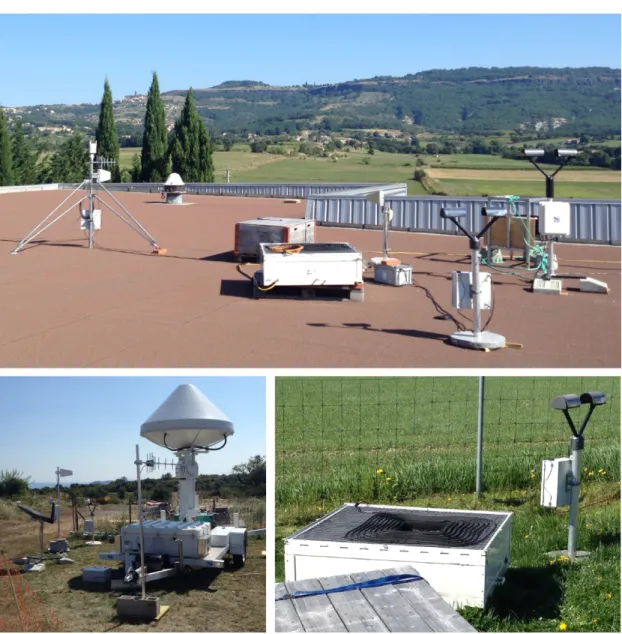
1.1 Examples of instruments deployed in the field . . . 9
2.1 Map of HyMeX station locations . . . 19
2.2 Distributions of drop diameters in HyMeX SOPs 2DVD data . . . 23
2.3 Proposed filter to remove non-physical measurements from Parsivel data . . . 25
2.4 Possible ranges of drop velocity interquartile range for 2DVD and Parsivel . . . 27
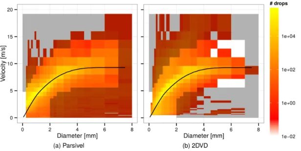
2.5 Parsivel and 2DVD drop velocity/diameter comparison . . . 28
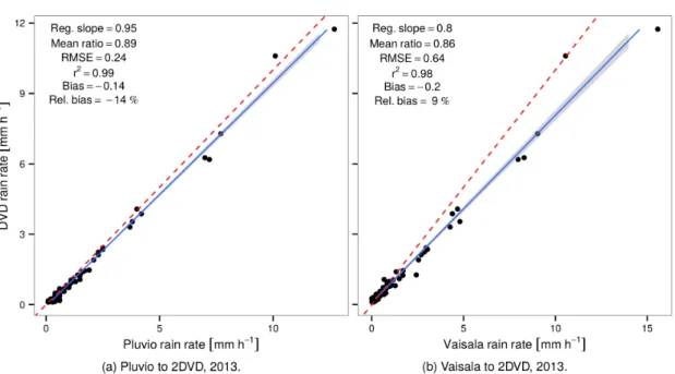
2.6 2DVD and Vaisala performance in HyMeX SOP2013 . . . 29
2.7 Example of velocity correction on Parsivel data . . . 30
2.8 Median Parsivel correction factor by Parsivel rain intensity . . . 32
2.9 Parsivel correction factor distributions by Parsivel-derived intensity . . . 33
2.10 Sampling effect on Parsivel correction factor by drop diameter class . . . 34
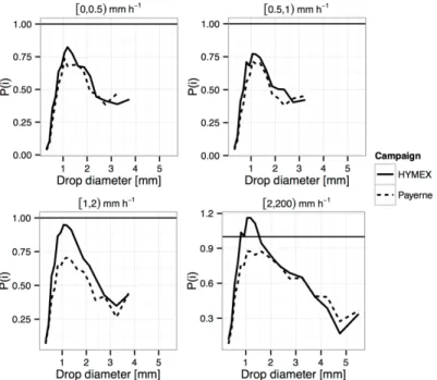
2.11 Parsivel correction factors for corrected DSDs . . . 35
2.12 Effect of Parsivel correction on DSD moments, densities . . . 36
2.13 Effect of Parsivel correction on DSD moments, Q-Q plots . . . 37
2.14 Parsivel correction effect onRat Pradel 1 station . . . 38
2.15 Comparison of first-generation Parsivel and Parsivel2correction factors . . . . 40
2.16 Comparison of Parsivel correction factors for different field campaigns . . . 41
3.1 Experimental dry drifts for the third disdrometer diameter class, all events . . . 63
3.2 Experimental dry drifts for the 17th disdrometer diameter class, all events . . . 64
3.3 Experimental dry drifts for example event . . . 66
3.4 Fitted dry drift models for example event . . . 67
3.5 Symmetry of DSD principal component distributions . . . 68
3.6 Examples of variograms per DSD principal component . . . 70
3.7 Example DSD interpolation:Rand its estimation interquartile range . . . 71
3.8 Example DSD interpolation:Dmand its estimation interquartile range . . . 72
3.9 Example DSD interpolation:ZH and its estimation interquartile range . . . 73
3.10 Leave-one-out bias on interpolated drop concentrations . . . 73
3.11 Leave-one-out relative error on interpolated drop concentrations . . . 74
3.12 Leave-one-out relative error on DSD bulk variables . . . 74
3.13 Example stochastically simulated rain rate realisations . . . 75
4.1 Regions of interest corresponding to real-world areal pixel sizes . . . 88
4.2 Example of stochastically simulated realisations of radar reflectivity . . . 90
4.3 Look-up table results for determiningDmfrom polarimetric information . . . . 92
4.4 Distributions of simulated point to areal DSD absolute error . . . 98
4.5 Interquartile ranges of relative errors in point to areal DSD comparisons . . . . 99
4.6 Distributions of point to areal DSD relative error in three drop size classes . . . 99
4.7 Distributions of point to areal DSD relative error by point rain rate . . . 100
4.8 Distributions of point to areal bulk variable relative error . . . 101
4.9 Distributions of point to areal bulk variable relative error, by point rain rate . . 103
4.10 Interquartile ranges of point to areal relative errors on DSDs, by areal size . . . 104
4.11 Interquartile ranges of point to areal bulk variable relative errors, by areal size . 104 4.12 GPM-derived compared to DSD-derived rain rate for areal DSDs . . . 106
4.13 GPM-derived compared to DSD-derived bulk variables for areal DSDs . . . 106
4.14 GPM DSD parameterµcompared to that fitted to simulated areal DSDs . . . . 107
4.15 COSMO-derived compared to DSD-derived rain rate for areal DSDs . . . 107
4.16 COSMO-derived compared to DSD-derived bulk variables for areal DSDs . . . 108
4.17 COSMO DSD parameters compared to those fitted to simulated areal DSDs . . 109
4.18 Total rain amounts by support and method . . . 110
4.19 Histogram of sampled areal rain rates . . . 110
5.1 Differences in normalised and measured DSDs with horizontal displacement . 121 5.2 Differences in normalised and measured DSDs with vertical displacement . . . 122
5.3 Examples of normalised DSDs per station for disdrometer data . . . 123
5.4 Examples of normalised DSDs per altitude for MXPol data . . . 123
5.5 Normalised DSD model performance through horizontal displacement . . . 125
5.6 Normalised DSD model performance through vertical displacement . . . 125
5.7 Median relative bias in reconstructed DSDs, by input moment combination . . 127
5.8 Percentage of variance unexplained, by input moment combination . . . 127
6.1 Fitted relationship between radar reflectivity and DSD moment six . . . 137
6.2 Time series of measured and retrieved rain rates . . . 139
6.3 DSD-retrieval scatter plots for HyMeX Parsivel data . . . 140
6.4 DSD-retrieval method performance comparison for HyMeX Parsivel data . . . . 140
6.5 Performance differences between DSD-retrieval techniques on Parsivel data . . 147
6.6 DSD-retrieval results compared to MRR-estimated DSDs aloft . . . 148
6.7 DSD-retrieval results compared to Parsivel DSDs . . . 148
6.8 Performance differences between DSD-retrieval techniques on real radar data . 149 7.1 The 2D-video-disdrometer in the Swiss Alps . . . 157
7.2 Densities of estimated snow-flake mass . . . 159
7.3 Examples of reconstructed snow mass columns . . . 160
7.4 Reconstructed and homogeneously distributed snow mass columns . . . 161
List of figures
7.6 Examples of snowflake accumulation maps . . . 163
7.7 Example spectral analyses for reconstructed vertical columns . . . 165
7.8 Example TM and DTM analyses for reconstructed vertical columns . . . 165
7.9 Example spectral analyses for snowfall time series . . . 168
7.10 Example TM analyses for snowfall time series . . . 168
7.11 Example spectral analyses for snow accumulation maps . . . 169
List of tables
2.1 HyMeX station locations and information . . . 20
2.2 HyMeX SOP2013 2DVD clock adjustments . . . 21
2.3 Parsivel drop diameter classes containing recorded raindrops . . . 24
2.4 Large drops recorded by 2DVD in HyMeX . . . 25
2.5 First-generation Parsivel correction factors for HyMeX SOP2013 . . . 31
2.6 Parsivel correction performance by moment order at Pradel Grainage (5 min) . 32 2.7 Parsivel correction effects for HyMeX SOP2012 (5 min) . . . 38
2.8 Parsivel correction effects for HyMeX SOP2013 (5 min) . . . 39
2.9 Parsivel correction effects for HyMeX combined SOPs (5 min) . . . 39
2.10 Parsivel performance for combined SOPs before correction (5 min) . . . 40
2.11 Parsivel performance for combined SOPs after correction (5 min) . . . 40
2.12 Parsivel correction effects on DSD moments for HyMeX (1 hour) . . . 42
2.13 Parsivel correction effects on one hour rain rate . . . 42
2.14 Calibrated Parsivel2correction factors for HyMeX SOP2013 . . . 43
2.15 Parsivel correction effects on HPicoNet data (1 hour) . . . 44
2.16 Parsivel2correction effects on DSD moments (1 hour) . . . 44
2.17 Calibrated Parsivel correction factors for Payerne . . . 45
2.18 Parsivel correction effects for Payerne . . . 45
2.19 Parsivel correction effects on DSD moments for Payerne (10 min) . . . 46
2.20 Parsivel correction effects on DSD moments for Payerne (1 hour) . . . 46
2.21 HyMeX correction effects on DSD moments for Payerne (10 min) . . . 47
3.1 HyMeX 2012 and 2013 rainfall events . . . 61
3.2 Hours of rainfall and rainfall amounts within-events, per station . . . 62
3.3 Dry drift model parameters for example events . . . 66
3.4 PCA component properties for example event . . . 67
3.5 Leave-one-out errors on bulk variables from interpolated DSDs . . . 72
4.1 Absolute error of point compared to areal DSDs (2.8×2.8 km2) . . . 94
4.2 Relative error of point compared to areal DSDs (2.8×2.8 km2) . . . 95
4.3 Absolute error of point compared to areal DSDs (5×5 km2) . . . 96
4.4 Relative error of point compared to areal DSDs (5×5 km2) . . . 97
4.6 Point to areal absolute errors on bulk variables by areal size . . . 101
4.7 Point to areal relative errors on bulk variables by areal size . . . 102
4.8 Linear models for interquartile range of point to areal difference by areal size . 105 5.1 Studied HyMeX rainfall events and estimated freezing levels . . . 117
5.2 Station coordinates for three instrument networks . . . 118
5.3 Fitted normalised DSD model parameters by input moment combination . . . 126
6.1 Instrument stations and corresponding PPI scan volumes . . . 136
6.2 Fitted coefficients for prediction of DSD moment three . . . 138
6.3 DSD-retrieval performance for simulated radar variables in HyMeX data set . . 141
6.4 DSD-retrieval performance differences for simulated radar variables . . . 142
6.5 Mean differences in DSD-retrieval performance on simulated radar data . . . . 143
6.6 Fitted coefficients for prediction ofZDRandKdp . . . 144
6.7 DSD-retrieval method performance differences using real radar data . . . 146
7.1 Studied one-hour portions of snowfall events . . . 158
7.2 Numbers of snowflake accumulation maps found . . . 163
7.3 Multifractal analysis results for reconstructed vertical columns . . . 164
7.4 Multifractal analysis results for homogeneous vertical columns . . . 166
7.5 Multifractal analysis results for snowfall time series . . . 169
List of symbols
a range-defining parameter of dry drift model [m] . . . 63
A set of points in which a process is active . . . 153
Ac area of ellipse/circle that covers a snowflake [m2] . . . 158
Ae area of pixels covered by a snowflake [m2] . . . 158
BA bulk variable defined on areal scale . . . 91
BP bulk variable defined on point scale . . . 91
c generalised gamma model parameter [–] . . . 116
c0 dry drift model nugget [–] . . . 63
cd dry drift model (partial) sill [–] . . . 63
cD fractal co-dimension function . . . 154
C constant for estimation ofKdp[–] . . . 134
C1 mean intermittency [–] . . . 154
Cn DSD-normalisation constant for moment ordern[–] . . . 115
Cv,i drops recorded forvth velocity class andith diameter class [–] . . . 22
CF fractal co-dimension [–] . . . 153
C principal components matrix . . . 55
C∗ matrix of estimated components . . . 58
d a distance [m] . . . 64
d² spatial dimension of a field²[–] . . . 153
d0 zero distance in Gaussian dry drift model [m] . . . 64
d(z) distance from locationzto nearest dry point [m] . . . 53
D equivolume raindrop diameter [mm] . . . 4
DF fractal dimension [–] . . . 153
Di class-centre diameter ofith drop diameter class [mm] . . . 22
Dk class-minimum diameter ofkth drop diameter class [mm] . . . 52
Dm mass-weighted mean drop diameter [mm] . . . 5
Dmax maximum considered drop diameter [mm] . . . 6
Dmin minimum considered drop diameter [mm] . . . 6
D0 median volume drop diameter [mm] . . . 5
e a moment order [–] . . . 154
es maximum moment order [–] . . . 154
E expectation . . . 54
EB relative point-to-areal difference on bulk variable [%] . . . 91
ER relative point-to-areal difference on drop concentration [%] . . . 91
Et difference (observed−reference) for timet . . . 26
fhh Forward scattering amplitude in horizontal polarisation [cm] . . . 134
fv v Forward scattering amplitude in vertical polarisation [cm] . . . 134
fG Gaussian dry drift model . . . 65
fk dry drift function for thekth diameter class . . . 54
fS spherical dry drift model . . . 64
FN normalised DSD model shape factor [–] . . . 83
F the Fourier transform . . . 156
g acceleration due to gravity [m s−2] . . . 158
h(x) double-normalised DSD [–] . . . 115
ˆ
h(x) generalised gamma function as a fitted double-normalised DSD [–] . . . 116
H degree of non-conservation [–] . . . 154
i the complex unit . . . 156
I a mean-normalised field . . . 156
Ib Nw-normalised reflectivity [dB] . . . 85
Ie normalised specific attenuation [dB km−1mm m3] . . . 85
I(z) binary rainfall occurrence for locationz[–] . . . 53
k specific attenuation [dB km−1] . . . 84
K moment scaling function . . . 154
Kdp specific differential phase shift [◦km−1] . . . 134
ˆ
Kdp estimatedKdp[◦km−1] . . . 134
|Kω|2 dielectric factor of water [–] . . . 5
l a distance lag . . . 56
l² observation scale of a field². . . 153
L number of spatial locations [–] . . . 55
L² outer scale of a field². . . 153
m the mass of a snowflake [g] . . . 158
M number of drops recorded within integration time [–] . . . 22
Mn DSD moment of ordern[mmnm−3] . . . 115
ˆ
Mn estimated DSD moment of ordern[mmnm−3] . . . 137
M matrix of log-transformed and detrended drop concentration measurements . 55
M∗ estimated detrended drop concentrations matrix . . . 58
˜
M normalised version ofM. . . 55
˜
M∗ estimated normalised detrended concentrations matrix . . . 58
Mk mean ofkth column inM[–] . . . 55
N0 intercept parameter of gamma DSD model [mm−1−µm−3] . . . 83
NA areal estimate of drop concentration [mm−1m−3] . . . 91
Ni volumetric drop concentration forith diameter class [mm−1m−3] . . . 22
Nl number of samples pairs of points for distance lagl[–] . . . 56
List of symbols
Nκ,A number of boxes to cover process points in fieldAand resolutionκ[–] . . . 153
NP point estimate of drop concentration [mm−1m−3] . . . 91
Nt total drop concentration [m−3] . . . 4
Nw scaling factor of normalised DSD model [mm−1m−3] . . . 83
N∗ estimated volumetric drop concentration [mm−1m−3] . . . 58
˜
N log-transformed drop concentration [–] . . . 53
˜
N∗ estimated log-transformed drop concentration [–] . . . . 58
N† detrended, log-transformed drop concentration [–] . . . 54
N†∗ estimated detrended, log-transformed drop concentration [–] . . . 58
N(D) volumetric drop size distribution [mm−1m−3] . . . 4
Ot observed value for timet . . . 26
p a power to analyse [–] . . . 160
P number of particles considered [–] . . . 160
Pl length of Parsivel laser sheet [mm] . . . 21
Pw width of Parsivel laser sheet [mm] . . . 21
P(i) correction factor for theith Parsivel diameter class [–] . . . 30
q total mass fraction of water [–] . . . 86
Qs contribution to total variance bysth principal component [–] . . . 55
r2 Pearson’s correlation coefficient [–] . . . 26
rm mass-weighted mean raindrop axis ratio [–] . . . 134
rz reflectivity-weighted mean drop axis ratio [–] . . . 133
R rain rate/intensity [mm h−1] . . . 4
˜
Rp measure of precipitation intensity, powerp[mmph−p] . . . 161
Rt reference value for timet . . . 26
R2DVD rain rate calculated drop-wise for 2DVD [mm h−1] . . . 22
Re Reynold’s number [–] . . . 159
S number of principal components [–] . . . 55
S2DVD effective 2DVD sampling area [m2] . . . 21
SPars effective Parsivel sampling area [m2] . . . 21
T number of time steps [–] . . . 26
U number of drop diameter classes [–] . . . 55
Vi class-centre velocity ofith velocity class [m s−1] . . . 22
v(D) terminal still-air fall velocity of a raindrop [m s−1] . . . 4
Vf particle velocity [m s−1] . . . 159
w wave number [–] . . . 155
wr kriging weight for therth location [–] . . . 57
W liquid water content [g m−3] . . . 4
W principal components transformation matrix . . . 55
x second-normalised drop diameter [–] . . . 115
X Davies number [–] . . . 159
Xp snowfall mass quantity, powerp[gp] . . . 160
Xs∗ estimatedsth principal component value [–] . . . 57
z a spatial location . . . 52
z0 the estimation location . . . 57
zr therth location . . . 57
Z radar reflectivity [dBZ] . . . 5
ZDR differential reflectivity [dB] . . . 6
ˆ
ZDR estimatedZDR[dB] . . . 143
Zh radar reflectivity in horizontal polarisation [mm6m−3] . . . 6
ZH radar reflectivity in horizontal polarisation [dBZ] . . . 5
Zl radar reflectivity (linear units) [mm6m−3] . . . 85
Zv radar reflectivity in vertical polarisation [mm6m−3] . . . 6
ZV radar reflectivity in vertical polarisation [dBZ] . . . 5
α multifractality index [–] . . . 154
αK coefficient for estimation ofKdp. . . 144
αM coefficient for estimation ofM3. . . 138
αZ coefficient for estimation ofZDR. . . 143
β spectral slope [–] . . . 155
βK1 first exponent for estimation ofKdp. . . 144
βK2 second exponent for estimation ofKdp. . . 144
βM exponent for estimation ofM3. . . 138
βZ exponent for estimation ofZDR. . . 143
δ diameter class width [mm] . . . 4
∆t measurement integration time [s] . . . 22
² data field . . . 153
ˆ
² normalised fractionally integrated field . . . 156
˜
² unnormalised fractionally integrated field . . . 156
η a power [–] . . . 155
ηair air viscosity [kg m−1s−1] . . . 158
γZ variogram for processZ . . . 56
Γ the gamma function . . . 116
˜
γs Cressie sample variogram . . . 57
κ resolution of a field [–] . . . 153
λ radar wavelength [cm] . . . 5
Λ slope parameter of gamma DSD model [mm−1] . . . 83
µ shape parameter of gamma DSD model [–] . . . 83
Ω set of dry locations . . . 61
ψ a multifractal singularity [–] . . . 154
ψs maximum singularity [–] . . . 154
ρ total density of air/water mixture [g cm−3] . . . 86
ρa air density [g cm−3] . . . 86
ρω density of water [g cm−3] . . . 4
List of symbols
σbH back-scattering cross-section, horizontal polarisation [cm
2] . . . . 5
σbV back-scattering cross-section, vertical polarisation [cm
2] . . . . 6
σe extinction cross-section [cm2] . . . 84
σ(Mk) standard deviation ofkth column inM[–] . . . 55
List of acronyms
2DVD two-dimensional video disdrometer . . . 6
COSMO consortium for small-scale modelling . . . 9
DSD (rain)drop size distribution . . . 1
DFIR double fence intercomparison reference . . . 157
DFR dual-frequency ratio . . . 85
DPR dual-frequency precipitation radar . . . 84
DTM double trace moment . . . 155
EPFL École Polytechnique Fédéral de Lausanne . . . 18
LTE Laboratoire de Télédétection Environnementale . . . 18
GPM global precipitation measurement . . . 10
GPS global positioning system . . . 19
HPE heavy precipitation event . . . 10
HyMeX Hydrological Cycle in the Mediterranean Experiment . . . 11
IQR interquartile range . . . 29
IFloodS NASA Iowa Flood Studies . . . 117
KED kriging with external drift . . . 50
MCS mesoscale convective system . . . 10
MRR micro rain radar . . . 7
NWP numerical weather model . . . 3
NASA National Aeronautics and Space Administration . . . 117
ORB orographic rain band . . . 10
Parsivel particle size and velocity (disdrometer) . . . 6
PCA principal component analysis . . . 51
PPI plan position indicator . . . 62
PVU percentage of variance unexplained . . . 126
QPE quantitative precipitation estimation . . . 2
radar radio detection and ranging . . . 2
RB (median) relative bias . . . 26
RMSE root mean squared error . . . 26
ROI region of interest . . . 89
RSE residual standard error . . . 126
SNR signal to noise ratio . . . 60
SCOP-ME SCOP attenuation correction and microphysics estimation . . . 133
SOP special observation period . . . 18
TM trace moment . . . 155
TRMM tropical rainfall measuring mission . . . 2
US United States . . . 80
UM universal multifractal . . . 13
UTC coordinated universal time . . . 25
UTM universal transverse Mercator . . . 89
1
Introduction
Precipitation is a profoundly important process. As a primary part of the Earth’s hydrological cycle, it delivers fresh water to the land, dramatically shapes the landscape, and is crucial to sustaining life. Liquid precipitation is rain, and its extremes have significant impacts: droughts and floods threaten life and property (e.g. Pielke Jr and Downton, 2000) and have substantial societal and economic effects (e.g. Ciais et al., 2005). Climate change is likely to change the frequency, intensity, and duration of rainfall events (Easterling et al., 2000; Trenberth et al., 2003; Stocker et al., 2013). It is expected that most land areas will experience an increase in the frequency of heavy rainfall events by the end of this century (Stocker et al., 2013). Accurate measurement is the key to being able to understand, model, and predict precipitation, including rain. Precipitation is not an easy process to measure, however, because it is notoriously variable. This variability exists on large scales (e.g. Koster and Suarez, 1995), which is why we experience wet and dry summers, or flooding in one region while another is unscathed. But precipitation is also highly variable at the small scale (e.g. Fabry, 1996), down to the scale of individual falling water particles. These particles, called hydrometeors, exist in many different phases, shapes, and sizes. The study of precipitation microphysics, or the dynamics of precipitation at the particle scale, leads to improved understanding of related processes across scales. The aim of this thesis is to contribute to the understanding and characterisation of the small-scale variability of rainfall.
Rainfall, of course, is made up of falling drops of water. When we speak of small-scale vari-ability of rainfall, what is meant is varivari-ability in the number of raindrops there are, and in their sizes. Because it is unfeasible to count and measure every single raindrop in a storm, statistics are used to summarise the information into a form that is more convenient to deal with. The raindrop size distribution (DSD) statistically describes the microstructure of liquid precipitation. It is defined as the number of falling raindrops of a certain size per unit volume of air. All rainfall variables of interest can be calculated as weighted statistical moments of the DSD (e.g. Ulbrich, 1983; Testud et al., 2001). These include the total drop concentration, the characteristic drop diameter, the liquid water content, and the rain intensity. Information about the DSD is needed to calculate the interactions of electromagnetic waves with
inho-mogeneous collections of hydrometeors in the atmosphere, making DSD properties required knowledge for weather radar applications (Marshall et al., 1947; Bringi and Chandrasekar, 2001). While the DSD describes what is happening at the raindrop scale, it is fundamental to processes that occur on much larger scales (e.g. Uijlenhoet and Sempere Torres, 2006). It is used in investigations into rainfall microphysical processes (e.g. Rosenfeld and Ulbrich, 2003); interactions of raindrops with surface soil (e.g. van Dijk et al., 2002), vegetation canopies (e.g. Calder, 1986), and built environments (e.g. Blocken and Carmeliet, 2004); the cleaning effect rain has in removing aerosols from the atmosphere (e.g. Andronache, 2004); weather prediction models (e.g. Baldauf et al., 2011); and the effects of rainfall on telecommunication links (e.g. Crane, 1971; Schleiss and Berne, 2010).
Since the discovery that the power of electromagnetic radiation reflected off rain relates to the rain’s intensity (Marshall et al., 1947), weather radar (radio detection and ranging) has revolutionised the measurement of precipitation. Marshall et al. (1947) foresaw the possibility of quantitative precipitation estimation (QPE) in the 1940s. In the 1970s, it was recognised that polarimetric radar, in which the waves are vertically and horizontally polarised, could offer greater insight into precipitation microstructure (Seliga and Bringi, 1976). Nowadays, radar has become an essential tool for the study of precipitation (Bringi and Chandrasekar, 2001; Berne and Krajewski, 2013), and operational networks provide near-real-time precipitation observations in many countries (e.g. Berne and Krajewski, 2013). Radars do not measure the rain intensity directly, but rather they make indirect and integrated measurements of the electromagnetic properties of hydrometeors in a measurement volume (Berne and Kra-jewski, 2013). The basic problem in QPE is determining the relationship between the radar measurements and the rain rate in the measured volume.
Conventional radars measure radar reflectivityZ (measured in mm6m−3but often expressed
in dBZ), which is non-linearly related to the rain rateR[mm h−1] via the DSD (e.g. Marshall
and Palmer, 1948; Uijlenhoet, 2001). TheZ–Rrelationship is usually modelled as a power law
that is scale dependent (Verrier et al., 2013; Sassi et al., 2014) and affected by DSD variability (Chapon et al., 2008; Jaffrain and Berne, 2012a). Polarimetric radars measure the reflectivity and phase change of horizontally and vertically polarised waves, and use this information to
retrieve DSD properties (Krajewski and Smith, 2002). In both cases, determiningRfrom radar
measurements is made complex by sampling issues (e.g. Andrieu et al., 1997), comparisons of incompatible scales, and instrumental uncertainty (Krajewski and Smith, 2002). With the advent of satellite-based weather radars (e.g. Kawanishi et al., 2000; Hou et al., 2014) and passive sensors, precipitation can now be observed on a global scale (e.g. Huffman et al., 2007; Hou et al., 2008). Algorithms for satellite-based QPE generally use a model of the DSD with parameters that are either fixed or derived from observations (e.g. Iguchi et al., 2000; Seto et al., 2013; Liao et al., 2014). The assumption of the DSD from a model was classed as a primary uncertainty factor for the Tropical Rainfall Measuring Mission (TRMM) satellite weather radar (Iguchi et al., 2009). Variability in the DSD affects the accuracy of radar observations of rainfall, whether they are made from the ground or from space.
1.1. The raindrop size distribution
Improving our understanding of the DSD and its small-scale variability will lead to better understanding of the physical processes at play in rainfall, reduced uncertainty in precipitation measurements, and more accurate numerical weather prediction (NWP). In this thesis we present new techniques for the measurement and stochastic simulation of the DSD, and we use them to quantify DSD variability and test DSD-retrieval techniques in Mediterranean rainfall. This introductory chapter sets the scene for the rest of the thesis, by briefly introducing the main topics and outlining the current state of the art. In Section 1.1 the DSD and its related bulk variables are introduced in more detail. Measurement and estimation of the DSD are discussed in Section 1.2. The effects of DSD variability and the change of support problem are discussed in Section 1.3. The bulk of the data used in this thesis were collected in Ardèche, France, a region that experiences heavy Mediterranean rainfall. The meteorological processes of this region are briefly introduced in Section 1.4. In Section 1.5, the outline of the rest of the thesis is shown.
1.1 The raindrop size distribution
Let us imagine a rainstorm, frozen in time. We take one cubic metre of space within the storm, and within this space we collect all the raindrops, count them and measure their sizes.
On average, there would be about 103falling raindrops in this cubic metre (Uijlenhoet and
Sempere Torres, 2006). Most of the drops would be small, between about 0.1 and 1 mm in diameter, and close to spherical (Pruppacher and Klett, 2000). There would also be some larger drops, which would be affected by air resistance, and thus not spherical. The bottom of these drops flattens, giving them an oblate shape that can be predicted as a function of the drop’s volume (e.g. Beard and Chuang, 1987; Andsager et al., 1999; Pruppacher and Klett, 2000; Thurai and Bringi, 2005; Thurai et al., 2007). Because not all raindrops are spherical, we speak of their size in terms of their equivolume diameter: the diameter of a sphere that contains the same amount of water as the drop. The great majority of raindrops have equivolume diameters between 0.1 and 6 mm (Uijlenhoet and Sempere Torres, 2006).
Now in our imaginary situation, let us allow the system to fall into motion. Each drop falls at a velocity that depends on its mass plus atmospheric conditions. The still-air terminal velocity of raindrops can be accurately predicted (e.g. Atlas et al., 1973; Beard, 1976; Brandes
et al., 2002) and ranges from 0.1 to more than 9 m s−1(Uijlenhoet and Sempere Torres, 2006;
Roe, 2005). As the rain falls, the number and sizes of the drops in our cubic metre of air are constantly changing. Evaporation causes the loss of some (mostly small) drops (e.g. Rosenfeld and Ulbrich, 2003). Drops collide with each other, with smaller drops joining together and coalescing to form larger drops, and larger drops breaking up (e.g. Pruppacher and Klett, 2000). Raindrops can only reach a certain size – about 10 mm – before they break up into smaller drops solely due to aerodynamic forces (Pruppacher and Klett, 2000), and it is for this reason that there are always more small drops than larger ones.
writtenN(D) [mm−1m−3] , is the number of raindrops with equivolume diameter in the range
[D,D+δ) mm, per unit volume of air (Marshall and Palmer, 1948). The DSD describes the
microstructure of liquid precipitation. Integral parameters of rainfall, also known as bulk rainfall variables, can be derived as weighted moments of the DSD (e.g. Ulbrich, 1983; Testud
et al., 2001). Any bulk variablePcan be expressed as
P=aP
∞
Z
0
wPDpN(D)d D, (1.1)
wherepandapare constants andwpis a weight that may depend onD(Ulbrich, 1985). In
this section the most commonly used bulk variables are briefly defined in increasing moment order (for a detailed review, see e.g. Bringi and Chandrasekar, 2001).
The zeroth moment of the DSD is the total drop concentrationNt[m−3], defined simply as
Nt= ∞
Z
0
N(D)d D. (1.2)
The DSD can be expressed as the total drop concentration multiplied by a probability density
function f(D) [mm−1], such thatN(D)=Ntf(D). The liquid water content,W [g m−3] is
related to the third moment of the DSD:
W =π10 −3ρ ω 6 ∞ Z 0 D3N(D)d D, (1.3)
whereρω[g cm−3] is the density of water. The flux of rainwater at a surface is expressed by the
rain rateR[mm h−1], defined as
R=6π10−4
∞
Z
0
N(D)v(D)D3d D, (1.4)
wherev(D) [m s−1] is the still-air fall velocity for a drop with equivolume diameterD. For the
work presented in this thesis, we used the model of Beard (1976) to calculatev(D).Ris the
1.1. The raindrop size distribution
The median-volume drop diameter,D0[mm], is the diameter that divides the DSD into two
portions of equal water volume. More commonly used as a characteristic drop diameter,
however, is the mass-weighted mean drop diameter,Dm [mm]. It is defined as the fourth
divided by the third moment of the DSD, such that
Dm= ∞ Z 0 D4N(D)d D ∞ Z 0 D3N(D)d D . (1.5)
Weather radars emit electromagnetic radiation and measure what is reflected back off hydrom-eteors in the atmosphere. Radar reflectivity, the quantity measured by conventional radars, can be derived from the DSD (Marshall and Palmer, 1948). When the particles scattering the radiation are much smaller than the radar wavelength, the scattering properties are governed
by the Rayleigh regime, and radar reflectivity Z [dBZ] is equal to the sixth DSD moment
(Marshall and Palmer, 1948; Bringi and Chandrasekar, 2001), such that
Z=10 log10 Dmax Z Dmin N(D)D6d D . (1.6)
It is often the case, however, that the particles are similar in size to the wavelength. In this case the reflectivity occurs in the Mie regime, and it can be calculated from the DSD using
Z=10 log10 106λ4 π5|Kω|2 ∞ Z 0 σb(D)N(D)d D , (1.7)
whereλ[cm] is the radar wavelength,|Kω|2[-] is the dielectric factor of water, andσb(D) [cm2]
is the back-scattering cross-section for a drop with equivolume diameterD(e.g. Bringi and
Chandrasekar, 2001). The scattering properties of water droplets can be calculated using the T-matrix codes of Mishchenko and Travis (1998).
In the case of polarimetric radars, in which the electromagnetic waves are horizontally and
vertically polarised, the horizontal reflectivityZH[dBZ] is calculated by replacingσb(D) in
Equation 1.7 withσb H(D) [cm2], the back-scattering cross section in horizontal polarisation.
[cm2], the back-scattering cross-section in vertical polarisation. It is common practice to refer to radar reflectivity in dBZ as defined above. At times it is also used, however, in its linear units,
in which case we have horizontal reflectivityZh[mm6m−3] and vertical reflectivityZv[mm6
m−3], defined asZ
h=10ZH/10andZv=10ZV/10respectively. Differential reflectivity,ZDR[dB],
defined asZH−ZV, is the ratio of horizontal to vertical reflectivity.ZDRis a useful variable in
rain, because with large drops being more oblate it is related to drop size (Seliga and Bringi, 1976).
In this section, all the integrals have been written assuming a continuous DSD function and drop sizes ranging from zero to infinity. This is idealised, because in reality, not only are drops finite in size, but they are usually measured in discrete classes of equivolume drop diameter. When working using measured data, therefore, the integrals in calculations of bulk variables
convert to sums over the drop size classes fromDmin[mm] toDmax[mm], the smallest and
largest considered class-centre drop sizes.d Dbecomes the width of each class, andDis the
centre diameter of each class. Studies on DSD truncation and the calculation of bulk variables have concluded that the effects of truncation are negligible as long as the included range of
diameters is large enough aroundD0(Willis, 1984; Ulbrich, 1985; Vivekanandan et al., 2004).
It is common for the DSD to be summarised using a functional form defined by only a few parameters. The first proposed form was the exponential function of Marshall and Palmer (1948). The Gamma DSD (Ulbrich, 1983) is an extension of the exponential form that is more appropriate for instantaneous measurements of the DSD. Other compact forms of the DSD include the normalised DSD of Willis (1984), and normalisation approaches in which the DSD is expressed using one or more of its statistical moments and a normalised DSD function that describes the shape of the distribution (e.g. Sempere-Torres et al., 1994; Testud et al., 2001; Lee et al., 2004). In this thesis we provide a DSD interpolation method that requires no functional form (Chapter 3), show results of using it to test areal rainfall retrieval functions that do use a DSD model (Chapter 4), and study the spatial invariance of a normalised DSD function (Chapter 5).
1.2 Measurement and estimation of the DSD
Disdrometers are instruments that measure the DSD at ground level, with collection areas that are small enough that they are usually considered to be point measurements. There are various types of disdrometers. Impact-type disdrometers (e.g. the Distromet Joss-Waldvogel disdrometer, Joss and Waldvogel, 1967) measure the impact forces of raindrops that hit a sensor. Laser optical disdrometers use a sheet of light that is interrupted by falling drops. The width of the shadow and length of the interruption give the size and fall speed of the observed particle. The primary data set used in this thesis is from a network of OTT Particle Size and Velocity (Parsivel, Löffler-Mang and Joss, 2000) laser optical disdrometers. Another type of disdrometer is the two-dimensional video-disdrometer (2DVD) (Schönhuber et al., 2008) that uses two orthogonally-facing cameras to take images of individual falling particles and to
1.2. Measurement and estimation of the DSD
directly measure their velocities. While the 2DVD has limitations (Tokay et al., 2001, 2013), it provides high-resolution data on individual hydrometeors, and matches rain rates from collocated rain gauges better than other disdrometers, including Parsivels (Tokay et al., 2001; Thurai et al., 2011; Tokay et al., 2013). Disdrometer data require careful treatment, because they can be affected by splashing, wind turbulence, multiple particles, particles that are not water (insects, spiderwebs), and instrumentation uncertainties (e.g. Kruger and Krajewski, 2002; Thurai and Bringi, 2005; Jaffrain and Berne, 2011; Tokay et al., 2013).
Networks of disdrometers have been the preferred way to study the variability of the DSD across space and time (e.g. Miriovsky et al., 2004; Lee et al., 2009; Tapiador et al., 2010; Tokay and Bashor, 2010; Jaffrain et al., 2011; Jameson et al., 2015a). A difficulty is that disdrometers provide point measurements that may be too sparsely distributed or not numerous enough to fully capture the variability of the rainfall process. It has been estimated that at least six disdrometers would be required per square kilometre to properly sample the variability of the DSD (Tapiador et al., 2010). Interpolation using geostatistics (Matheron, 1971; Chilès and Delfiner, 1999) offers a possible solution to this problem, through the estimation of the DSD at unmeasured locations, conditioned on nearby measurements. To date, rainfall interpolation methods that produce gridded outputs have generally worked with individual bulk variables such as rain rate (e.g. Creutin and Obled, 1982; Chua and Bras, 1982; Goovaerts, 2000; Tobin et al., 2011; Masson and Frei, 2014; Haberlandt, 2007; Velasco-Forero et al., 2008; Tobin et al., 2011). However, the full variability of the DSD can not be captured using only integral variables, because it is possible for multiple DSDs to produce the same bulk variable values (Jameson et al., 2015b).
Stochastic simulation can be used within a geostatistical framework to produce many equally probable realisations of a process. This approach has been used to estimate DSD model parameters and investigate DSD variability (Jaffrain and Berne, 2012b; Schleiss et al., 2012). The assumption of either second-order or at least intrinsic stationarity is required for geosta-tistical approaches (Chilès and Delfiner, 1999). Rainfall, however, is a non-stationary process (Barancourt et al., 1992; Schleiss et al., 2014a). This non-stationarity is caused largely by the high intermittency (patchiness) of rainfall fields (Schleiss et al., 2014a). While intermittency can be modelled through the use of a rainfall occurrence map (Barancourt et al., 1992), this does not solve the problem of the non-stationarity. Schleiss et al. (2014a) offered a solution through taking into account the so-called “dry-drift”, or the tendency of rainfall to be heavier at a point that is further from a dry region (Barancourt et al., 1992; Braud et al., 1994; Emmanuel et al., 2012).
The techniques mentioned so far in this section have included direct sampling of the DSD with disdrometers, and interpolation and simulation of DSD parameters in order to investigate horizontal variability. The DSD varies in the vertical, as well. Vertically profiling radars that measure the Doppler spectrum are able to infer some properties of the DSD at height, using measured fall speeds towards the radar. This is the method used by micro rain radars (MRRs, Peters et al., 2002, 2005; Tridon et al., 2011). A significant limitation of these methods is
that vertical wind and turbulence are ignored (Peters et al., 2002). Schleiss and Smith (2015) proposed a geostatistical technique that uses disdrometer time series from the ground, and radar data, to estimate 3D–time variograms for DSD model parameters. Retrieval of the DSD from (non-Doppler) polarimetric radar data has been a long-standing goal, but has
proven difficult. Some microphysical properties, such as the median drop diameterD0, can be
retrieved from polarimetric information (Seliga and Bringi, 1976). Since this was discovered, many DSD-retrieval methods have been developed to try to retrieve other properties of the DSD (e.g. Zhang et al., 2001; Gorgucci et al., 2002; Park et al., 2005b; Anagnostou et al., 2009, 2010; Thurai et al., 2012; Bringi et al., 2015; Kalogiros et al., 2013).
In this thesis we present new ways to correct possibly inaccurate measurements of the DSD (Chapter 2), and new ways to infer the DSD or its properties from nearby or remote measure-ments. A new geostatistical interpolation technique and stochastic simulation technique for the experimental (i.e. non-parametric) DSD is presented (Chapter 3), and we introduce a new DSD-retrieval technique that uses polarimetric radar data (Chapter 6). These techniques were developed using measurements of the DSD made with disdrometers and radars. The disdrometers used were Parsivel laser optical disdrometers and a 2DVD. The main data set, which is introduced in Chapter 2, was collected by a network of disdrometers collocated with rain gauges, plus a weather station, MRRs, and an X-band polarimetric weather radar (MXPol, see Schneebeli et al., 2013). Examples of these instruments deployed in the field are shown in Figure 1.1.
1.3 DSD variability and the change of support problem
The support of a measurement is the region in space over which is it taken. The change of support problem refers to the non-equivalence of measurements taken with different supports. DSD measurements are affected by the change of support problem because of the high variability of the DSD. DSD variability is known to be at least as great within rainfall events as between them (Tapiador et al., 2010; Jaffrain and Berne, 2012b), and it has been shown that the variability of the DSD is greater across larger domains than smaller ones (Jaffrain and Berne, 2012b; Jameson et al., 2015b), and to be greater for larger (and therefore rarer) drops than smaller ones (Jameson et al., 2015b). Variability is greater between measurements taken with short integration times, as compared to longer ones where the integration causes smoothing of the process (Jaffrain and Berne, 2012b; Tokay and Bashor, 2010). Given this high variability, an areal measurement of the DSD can therefore not be assumed to equal a point measurement. Yet, at times, only areal measurements or only point measurements are available. In this thesis we quantify the error introduced by assuming a point represents an area, and investigate whether areal rainfall retrieval algorithms properly represent the sub-grid DSD.
The sub-grid variability of the DSD affects the areal retrieval of rainfall. For example, in radar QPE, the properties of the link between radar reflectivity and rain intensity varies with the
1.3. DSD variability and the change of support problem
Figure 1.1 – Examples of instruments used in this thesis, as deployed in the field. The top panel shows Pradel Grainage in Ardèche, France, with (L–R) the Vaisala weather station, 2DVD, first-generation Parsivel and Parsivel2. Below left shows the Montbrun, also in Ardèche, with (L–R) the MRR, first-generation Parsivel, and MXPol. Below right shows Payerne Station SwissMetNet, in Payerne, Switzerland, with (L–R) the 2DVD and a first-generation Parsivel disdrometer.
DSD. As well as the scales of the measurements being different, any comparison betweenZ
aloft andRon the ground is subject to additional uncertainty due to the vertical evolution of
the rainfall (Zawadzki, 1975). The grid size of rainfall products varies. For example, a typical
ground-based weather radar pixel size is 1×1 km2(Berne and Krajewski, 2013). NWP models
typically use slightly larger pixels; for example the high-resolution Consortium for Small-scale
Modelling (COSMO)1atmospheric model uses an operational pixel size of 2.8×2.8 km2(in
Germany, Baldauf et al., 2011). Space-borne weather radars use a larger pixel size; for example 1Seehttp://www.cosmo-model.org.
the Global Precipitation Measurement (GPM) satellite has a footprint of about 5×5 km2(Hou et al., 2014). The rainfall retrieval algorithms used by systems such as GPM and COSMO rely on first deriving DSD properties such as model parameters, then calculating bulk variables. The change of support problem means that DSD properties derived at the areal scale may not always be representative of the sub-grid rainfall process.
1.4 Mediterranean rainfall
The region of Ardèche, in France, was the study region for most of the work in this thesis. The western Mediterranean, in which Ardèche is located, is plagued by heavy precipitation events (HPEs) that threaten both life and property (Delrieu et al., 2005; Nuissier et al., 2008). The broad meteorological conditions that cause these events are well understood at a synoptic scale (Nuissier et al., 2011), so forecasting of likely HPEs across a large region is relatively accurate. However, forecasting and modelling the precise location of an HPE and the amount of rainfall likely to result remain difficult problems (Ricard et al., 2012; Delrieu et al., 2005). For example, in 2002 an HPE in the Gard region of France cost 24 lives and 1.2 billion euros in damage, but warnings produced before and during the event significantly underestimated the expected rainfall amount, and the prediction error in the location of the cell was about 100 km (Delrieu et al., 2005). Improved understanding of the small-scale variability of rainfall is important for the reduction of these sorts of problems.
The atmospheric conditions that cause heavy precipitation events in the Mediterranean are well known (e.g. Miniscloux et al., 2001; Lin et al., 2001). They can be divided into three meteorological ingredients. First, large masses of warm, moist air in the lower atmosphere are produced by the Mediterranean Sea, particularly during the end of summer and the start of autumn (Miniscloux et al., 2001). Second, synoptic-scale systems push this air onto the land. Typically, an upper-level cold trough forms between the Atlantic and the Mediterranean, with low pressure over the Gulf of Biscay and high pressure over central Europe: this trough-ridge pattern generates a southerly flow that destabilises the warm air and pushes it northwards (Miniscloux et al., 2001; Ricard et al., 2012). Third, the mountainous landscape of the Mediter-ranean coast triggers convective activity and heavy rainfall follows (Delrieu et al., 2005). The heaviest rainfall is on the south-eastern flanks of mountainous regions which lie perpendicular to the airflow from the sea (Nuissier et al., 2008). The synoptic pattern is often quasi-stationary and slowly shifts to the east while maintaining similar conditions, thus leading to high rainfall totals because events can persist for several hours to days (Ricard et al., 2012).
Mediterranean HPEs can be classified as deep-convective or shallow-convective, or a mixture of these two types. At the deep-convective end of the classification are quasi-stationary mesoscale convective systems (MCSs), which form a characteristic V shape with convective cells continuously generated at the point of the V. A quasi-stationary MCS can generate up to 200-600 mm of rainfall in under 24 hours (Delrieu et al., 2005). At the shallow-convective end are orographic events, that in stable conditions form orographic rain bands (ORBs). These
1.5. Thesis outline
events are associated with stationary flow, and form stable and active bands of precipitation which are parallel to the direction of the wind and can last for several hours (Miniscloux et al., 2001; Godart et al., 2011). Typically, deep-convective events are temporally shorter, show more intermittency (“patchiness”), and have higher rain rates than shallow-convective events (Godart et al., 2011). Orographic rainfall is a complex process (Houze, 2012) and precipitation rates in mountainous regions remain poorly known as a result (Roe, 2005).
The Hydrological Cycle in the Mediterranean Experiment2(HyMeX, Drobinski et al., 2014;
Ducrocq et al., 2014) is a long-term, multi-disciplinary, international project that brings together teams of scientists with the common goal of providing better understanding of the complex water cycle of the Mediterranean. It has a particular emphasis on extreme and high-impact weather events such as HPEs. The main study region for this thesis was in Cévennes, France, in which an instrument network was deployed as part of HyMeX. The Cévennes region lies to the southeast of the Massif Central, and forms a large south-easterly facing slope to the sea, dissected by deep and narrow northwest to southeast valleys (Miniscloux et al., 2001; Godart et al., 2011). It is one of the five rainiest areas in the region (Nuissier et al., 2008). Rain occurs particularly during the autumn - there is a well defined precipitation maximum in October (Frei and Schär, 1998). The region is subject to HPEs (Ricard et al., 2012) and ORBs (Godart et al., 2011), with an average 7.6 days per year with rainfall over 150 mm (between 1967 and 2006, Ricard et al., 2012). Data from two autumn field campaigns in this region were used in this work.
1.5 Thesis outline
The work in this thesis follows a logical arc, from collection of accurate DSD data from a network of disdrometers, to technique development for the study of the variability of the DSD using spatial interpolation and stochastic simulation, to analysis of DSD variability in the horizontal and vertical. Here, a brief overview of the following chapters is provided. Each chapter has been adapted from a published or submitted research article.
Chapter 2 relates to collection of the high-quality and accurate point measurements of the DSD. Most of the DSD data used in this thesis were collected by a network of Parsivel disdrometers, which is introduced in this chapter. Like any instrument, disdrometers have collection errors that must be taken into account when their data are used. In particular, these disdrometers classify drops into “bins” of drop size, and may misestimate the number of drops in each class. In Chapter 2 we present a method for the correction of disdrometer data recorded using Parsivel disdrometers, that uses a 2DVD as a reference. In the first part of the method, drop velocities are corrected with reference to a theoretical model of raindrop terminal velocity. Second, raw disdrometer measurements are filtered to remove particles that are unlikely to be real drops. Third, concentrations per Parsivel diameter class are corrected such that on average they match those recorded by the 2DVD. The correction method improves the match
of DSD moments between the Parsivel and the 2DVD, and test results are shown in which, in the majority of cases, the Parsivel-derived rain rate was closer to that of a collocated rain gauge after the correction was applied. The corrected Parsivel data were then used for technique development and analyses of DSD variability.
In Chapter 3, we present a new method for spatial interpolation and stochastic simulation of experimental DSD spectra. Disdrometers such as Parsivels provide non-parametric ex-perimental DSD spectra in which concentrations are provided per drop diameter class. In a network of disdrometers, the DSD is measured at discrete point locations with varying inter-measurement distance. Our interpolation and simulation approach uses geostatistics to estimate or simulate the DSD, in the same non-parametric classes, at unmeasured points in space. Careful processing is required in order to comply with the assumptions of the geosta-tistical technique. Non-stationarity of the DSD field is taken into account using the dry-drift (Schleiss et al., 2014a), which we show exists on DSD concentrations. Principal component analysis is used to find uncorrelated components of the DSD, which are then interpolated or simulated for the requested points. A back-transformation process produces the estimates of the DSD. Results of leave-one-out testing show low bias on the estimated DSDs.
In Chapter 4, the data correction and DSD stochastic simulation techniques are brought together to investigate the small-scale variability of the DSD. In this chapter we report on a study in which simulated high-resolution grids of DSDs, conditional on measurements, were used to test the effects of DSD variability on areal rainfall retrieval. DSD variability is studied over two scales that were chosen for their similarity to areal scales used in rainfall products.
The first scale, 5×5 km2, is the ground footprint size of the Global Precipitation Measurement
(GPM) satellite weather radar. The second scale, 2.8×2.8 km2, is the size of a pixel in the
operational Consortium for Small-scale Modelling (COSMO) numerical weather model. The error introduced by assuming that a point measurement represents an areal measurement is quantified by areal size, and the retrieval algorithms for both GPM and COSMO are evaluated with respect to whether their pixel-scale results are representative of the sub-pixel process. In Chapter 5 we move to investigation of the double-moment normalisation of the DSD. Normalisation allows for the compact representation of the DSD and is also useful for the investigation of DSD variability, but it relies on the idea that the normalised DSD is the same everywhere. We show that the double-moment normalisation method of Lee et al. (2004) is effective at collapsing the DSD into a mean shape. We show the results of tests on the invariance of the double-normalised DSD in three climatic regions, through both horizontal and vertical displacement of the normalised DSD. This is the first test of the invariance of the normalised DSD in the vertical and the first over a large horizontal range of up to 100 km in one region. The normalised DSD trained in one region is shown to be applicable to another region more than 7000 km away.
In Chapter 6, the assumption that the normalised DSD is invariant is used to develop a new technique for the retrieval of the DSD from polarimetric radar data. The assumption