Optimization of (s, S) Inventory Systems with Random Lead Times and a Service Level Constraint

with Random Lead Times and a Service

Level Constraint

Sridhar Bashyam

j

_{Michael C. Fu}

KPMG Peat Marwick LLP, 2300 Clarendon Boulevard, Arlington, Virginia 22201 The Robert H. Smith School of Business, University of Maryland, College Park, Maryland 20742

A

major assumption in the analysis of (s, S) inventory systems with stochastic lead times is that orders are received in the same sequence as they are placed. Even under this assump-tion, much of the work to date has focused on the unconstrained optimization of the system, in which a penalty cost for unsatisfied demand is assigned. The literature on constrained optimi-zation, wherein a service level requirement needs to be met, is more sparse. In this paper, we consider the constrained optimization problem, where orders are allowed to cross in time. We propose a feasible directions procedure that is simulation based, and present computational results for a large number of test cases. In the vast majority of cases, we come within 5% of estimated optimality.

((s, S) Inventory Systems; Random Lead Times; Service Level Constraint; Constrained Simulation

Op-timization; Feasible Directions Search; Perturbation Analysis)

1. Introduction

The case of random lead times for (s, S) inventory sys-tems has been handled under the key assumption that orders arrive in the same sequence as they are placed (Ehrhardt 1984, Zipkin 1986, Zheng and Federgruen 1991). Specifically, if we define the following random variables:

W(t)Åinventory level (stock on hand minus backor-ders) at time t,

I(t)Åinventory position (W(t) plus outstanding or-ders) at time t,

LÅorder lead time,

D(tÉL)Ådemand during the interval (t, t/L],

then the analysis typically proceeds by first deriving the probability distribution of I(t) via renewal theory, and then using the equation

W(t/L)ÅI(t)0D(tÉL) (1)

to determine the probability distribution of W(t). Much of the work reported on (s, S) systems uses this infor-mation on I(t) and W(t) to find an (s, S) pair that

min-imizes (or approximately minmin-imizes) a cost function that, in addition to setup and holding costs, assigns a penalty cost on backlogged demand. A review of a large number of optimal and approximately optimal algo-rithms to carry out this unconstrained optimization can be found in Porteus (1988). However, if orders are al-lowed to cross—which, in general, would be the case when there are multiple suppliers—(1) is no longer valid, and even the above unconstrained problem ap-pears to become analytically intractable. To our knowl-edge, the literature does not report any work related to this more general problem.

In spite of the huge body of literature that has been developed on the cost minimization problem, it has been widely recognized that penalty costs, and in par-ticular, the cost of losing customer goodwill, are usually difficult to assess. It is largely a result of this that service level measures are very popular in practice (Lee and Nahmias 1993). Under this approach, the objective is to determine an (s, S) pair that minimizes a cost function, defined only in terms of setup and holding costs, subject

to the constraint that the solution satisfies a prescribed

level of customer service. Unfortunately, from an analyt-ical viewpoint, this constrained optimization problem in-troduces the additional difficulty of having to deal with the probability distribution of backlogged demand. The purpose of our work is to incorporate two critical features in the determination of optimal settings of (s, S):

• service level constraint, and

• general random lead times that allow for order crossings.

A review of the literature on service level constraints reveals that the two most relevant works are Schneider and Ringuest (1990) and Tijms and Groenevelt (1984). Schneider and Ringuest consider a periodic review sys-tem operating under ag-service level measure, where (1 0 g) is the fraction of demand on backorder each period. They construct a Lagrangian function, and pro-pose algorithms that give nearly exact solutions to the three first-order conditionsÌL/ÌuÅ0, whereLis the Lagrangian function, anduÅs, S, andl. However, they assume a fixed lead time.

On the other hand, Tijms and Groenevelt (1984) con-sider a general class of (s, S) models, covering both the periodic and continuous review cases, and allowing random lead times, though prohibiting order crossings. They compare their proposed approximation with ‘‘op-timal’’ results obtained from a Lagrangian method, car-ried out via a line search on the Lagrange multiplier. However, they assume that QÅS0s is predetermined

(e.g., via the EOQ formula), and focus only on the de-termination of the reorder level s.

Another limitation of these approaches is their range of validity: both explicitly assume that S0s be

suffi-ciently large compared to the average period demand

mD; in particular, that S0s¢1.50mD. While Schneider

and Ringuest suggest alternative schemes when this condition is violated, Tijms and Groenevelt specifically mention that their approximations are not warranted when this condition is violated. For example, if we ar-bitrarily fix the setup cost K Å36, and the per-period holding cost hÅ1, and if Q is computed using the EOQ formula, then their algorithm is valid only when the average demand per period is less than or equal to 32. Moreover, when orders are allowed to cross, our sim-ulation results indicate that the approximation methods might perform quite poorly.

In this paper, we consider a periodic review (s, S) inventory with random lead times that allow for orders to cross in time. We adopt the ‘‘fill-rate’’ service level measure used by Tijms and Groenevelt, defined as the fraction of demand that is met directly from stock on hand. Our objective is to determine values of s and Q ÅS 0s that minimize the average setup and holding

cost per period, subject to the constraint that the fill-rate is above a prescribed level. Due to the analytic intrac-tability caused by order crossings, we adopt a simulation-based approach to the problem. A review of the state of the art in optimization via simulation (Fu 1994b, see also Safizadeh 1990, and Jacobson and Schru-ben 1989) indicates that computationally efficient simulation-based gradient estimation methods have been developed for a variety of systems, which makes the use of gradient-based search methods a very viable tool to optimize analytically intractable models (another possible approach is response surface methodology). We use the gradient estimators of cost with respect to s and Q derived by Fu and Hu (1994) and also derive gradient estimators for the service level measure. De-tailed expositions on gradient estimation for (s, S) in-ventory systems can also be found in Fu (1994a) and Bashyam and Fu (1994) (see also the monographs by Ho and Cao 1991, Glasserman 1991, and Fu and Hu 1997 for more general coverage of gradient estima-tion).

In terms of simulation optimization algorithms, a rich body of literature exists for the unconstrained version of the problem (see, for example, L’Ecuyer et al. 1994), but the literature on constrained optimization with ‘‘noisy’’ constraints is limited. Since our problem’s ser-vice level constraint requires estimation of the serser-vice level measure by simulation, it falls into the latter cat-egory of problems. When the constraints are of known functional form, a number of solution techniques are available (Kushner and Clark 1978), but the only re-ported algorithm we know of that handles noisy con-straints is the Lagrangian approach in Kushner and Clark (1978). There are several reasons that motivate us to consider alternative solution methods. The most sig-nificant among these reasons is the fact that the La-grangian method guarantees a feasible solution only in the limit, which could be an unacceptable feature in practical application.

We propose an algorithm based on the feasible direc-tions approach from nonlinear programming. The al-gorithm has several desirable properties:

• It is a direct search process that is very amenable to fine control.

• It converges relatively quickly in a stable manner. • It gives the user several good feasible solutions as it evolves.

• It incorporates a simple but robust scheme for pa-rameter settings.

In computational experiments involving various de-grees of order crossings, our algorithm came within 5% of optimality in 95% of the cases, and within 2% of op-timality in 68% of the cases. In contrast, the analytical methods produced optimality gaps in excess of 10% for over 75% of the cases. Thus, we believe that we offer a computationally viable algorithm that satisfactorily handles the case of order crossing in instances where analytical models can be expected to perform very poorly.

The rest of the paper is organized as follows. In §2, we formally specify the model and define the problem of interest. In §3, we extend the analysis of Fu and Hu (1994) to derive PA gradient estimators of the service level measure with respect to s and Q. Readers inter-ested mainly in the optimization algorithm may skip this section without any loss in continuity. In §4, we describe the proposed optimization algorithm based on a feasible directions approach, including the incorpo-ration of some simple preprocessing ideas that provides the gradient search routine with a good starting point. Computational results on a large number of cases cov-ering various demand and lead time distributions are reported in §5. Section 6 contains concluding remarks and directions for further research.

2. Problem Definition

We consider an infinite horizon periodic review inven-tory system with continuous-valued i.i.d. demands and full backlogging. The basic sequence of events in each period is as follows: Orders are received at the begin-ning of the period, the demand for the period is sub-tracted out, then an order review is carried out at the end of the period. The inventory level in period n is de-fined as the on hand stock minus backorders, and

ob-served after demand subtraction, and the inventory

po-sition is the inventory level plus any outstanding orders.

We define the following:

DnÅdemand in period n, i.i.d. with p.d.f. g(·) and c.d.f. G(·),

InÅinventory position in period n,

WnÅinventory level in period n,

VnÅinventory level in period n before demand sub-traction (ÅWn/Dn),

YnÅdemand in period n not satisfied from on hand stock (Å(Dn0V ) ),/ /n

LiÅlead time of ith order placed,

hÅper period holding cost,

KÅper order setup cost,

uÅper unit order cost, where x/_{Åmax(x, 0).}

Ordering decisions are made according to the well-known (s, S) policy: If Inõs, an order for the amount S0Inis placed; otherwise, no action is taken. The lead times Li for orders placed are assumed to be integer

valued i.i.d. random variables. Under our convention, an order with lead time l placed in period n will arrive at the beginning of period n/l/1. As indicated in the introduction, the performance of the system will be evaluated by a cost function and a service level mea-sure, where the cost measure considers only setup and holding costs, and the service level measure tracks the extent of backlogging in the system. Defining the cost for a single period n by

/

CnÅhWn /I{Inõs}(K/u(S0I )),n

where I{·} is the indicator function, we define the ex-pected cost per period:

N

1

U

C

NÅE[C ]N ÅE

F G

∑

Cn , (2)

N_nÅ1

where CVNis the sample performance measure. The

ser-vice level measure is the fraction of the total demand that is not satisfied from on hand stock, the complement of the fill-rate measure considered in Tijms and Gro-enevelt (1984), given by

N

(nÅ1Yn

J

NÅE[J ], where JN NÅ₍N _D . (3)

nÅ1 n

Denoting

C

and

J

as the infinite horizon measures ob-tained by letting Nr`in the corresponding measures,

and defininguÅ(s, Q), the optimization problem is the following mathematical program (P):

min

C

(u)

/

u√R1R

subject to

J

(u)°b.

The gradient estimators of

C

and

J

with respect to s and Q play a central role in the simulation optimization algorithm we propose in §4. In the next section, we de-rive these estimators using the technique of perturba-tion analysis. Since the estimators forÌ

_C

/Ìs andÌ

_C

/ÌQ

have already been specified by Fu and Hu (1994), we focus here on extending their analysis to develop esti-mators forÌ

_J

/Ìs andÌ

_J

/ÌQ.

3. Gradient Estimation

In this section, we use the gradient estimation technique of perturbation analysis to derive sample path estima-tors forÌ

_J

N/Ìs andÌ

J

N/ÌQ. These estimators then

pro-vide estimates for the infinite horizon gradientsÌ

_J

/Ìs

andÌ

_J

/ÌQ by taking N sufficiently large. Although the

development here is largely self-contained, certain tech-nical details have been omitted (cf., e.g., Bashyam and Fu 1994). In addition, implicit in the use of the finite horizon gradients for the infinite horizon problem is the assumption of strong consistency, requiring the inter-change of two limits; although this interinter-change is not addressed here, the corresponding proofs for the aver-age cost function can be found in Fu and Hu (1994). The interested reader is also referred to the monograph by Fu and Hu (1997) for a more detailed exposition on the perturbation analysis techniques used in this section.

In our derivations, we will refer to a nominal path as a sample path operating at the nominal values of the parameters (s, Q), whereas a perturbed path will refer to a sample path operating with one of the values per-turbed, in particular (s/Ds, Q) in §3.1 and (s, Q/DQ)

in §3.2. To distinguish quantities in the respective paths, the perturbed parameter will be displayed explicitly, whereas the other parameter will be omitted, e.g., In(s)

vs. In(s/Ds) in §3.1, and In(Q) vs. In(Q/DQ) in §3.2.

Finally, all estimators take the limit as the perturbation goes to zero (Dsr0 orDQr0), so that in the actual implementation there is no perturbation; it is merely an artifact of the presentation of the derivations.

3.1. Estimation with Respect to s

By definition, we have

Ì

_J

N ÌE[J ]N E[J (sN /Ds)0J (s)]N

Å Ålim .

Ìs Ìs Dsr0 Ds

If both paths start with an initially ‘‘full’’ inventory (at the order-up-to level), and both are subjected to iden-tical sequences of demand sizes and lead times, then keeping Q fixed means that the two paths are offset from each other byDs, but are otherwise identical in

shape. In the context of perturbation analysis, we say that the event order sequences are identical, from which the dominated convergence theorem can be used to jus-tify that the interchange of limit and expectation oper-ations in

ÌE[J ]N ÌJN

ÅE

F G

(4)

Ìs Ìs

is valid, so that the infinitesimal perturbation analysis (IPA) estimatorÌJN/Ìs is an unbiased estimator ofÌ

_J

N/

Ìs. To derive an expression for the sample path

esti-mator, we note that for all n, s, andDs, dVn V (sn /Ds)ÅV (s)n /Ds, so Å1.

ds

Since Yn Å (Dn 0 we have by straightforward

/ /

V ) ,n

differentiation (NB: at the point Dn 0Vn/Å0, the

de-rivative technically does not exist, but this point occurs w.p. 0 since demands are continuous),

d _(D / /

0V ) if D 0V ú0,

n n n n

dYn_Å ds

ds

5

_{0 otherwise,}

and since Dnis independent of s, we have

/ _{01 if V ú0,} n d _(D / dVn 0V )Å 0 Å n n

H

ds ds _{0 otherwise.}

Combining the two results, we get

01 if Vnú0, Vn0Dnõ0, ÌYn

Å

H

Ìs _{0 otherwise,}

so from (3), it follows that

N

ÌJN (nÅ1ÌY /n Ìs

Å _N ,

which results in the following IPA estimator for Ì

_J

N/Ìs: Ì

J

_N É

N

_IPAÉ Å 0 , (5)

S D

_{Ìs (}N _D nÅ1 n IPA

where

N

IPAÅ {n° N: Vn ú0, Vn 0Dn õ 0}. The set

NIPA

contains those periods where the fraction of de-mand satisfied from on hand stock is strictly positive and less than 1. As can be seen, the IPA estimator given by (5) can be implemented very efficiently.

3.2. Estimation with Respect to Q

When Q is varied byDQ, the nominal path operates at s and S, whereas the perturbed path operates at s and S

/DQ. Now consider a nominal sample path such that

for some n, we have In(Q)Ås0dõs, whered√(0,

DQ), i.e., an order is placed in period n in the nominal

path. Then, in the perturbed path, we have In(Q/DQ)

Ås/DQ 0dús, i.e., no order is placed in period n

in the perturbed path. This indicates a change in the

or-dering sequence between the two paths, which typically

results in a significant change (of O(1)) in the perfor-mance measure. Under these conditions, an interchange of the kind specified in (4) is no longer valid, and the IPA estimator for this case is not unbiased by itself. As in Fu (1994), Bashyam and Fu (1994), and Fu and Hu (1994, 1997), we use smoothed perturbation analysis to de-rive an unbiased estimator. We begin by introducing some additional sample path notation:

UnÅ(In/Dn)Åinventory position in period n before

demand subtraction,

ZnÅUn0s,

enÅ

H

1 if an order is placed in the nth period, 0 otherwise,

O

n Å{e1(Q) Å e1(Q / DQ), . . . , en01(Q) Åen01 (Q /DQ), en(Q)xen(Q/DQ)}, Å{e1(Q)Åe1(Q/DQ), e2(Q)Åe2(Q/DQ), . . . , U

O

eN(Q)ÅeN(Q/DQ)},

h(n)Ånumber of orders placed up to and including period n,

H

nÅ{D1, D2, . . . , Dn01, L1, L2, . . . , Lh(n )}.

O

n defines the event that the first ordering sequence

change (depending on s, Q, andDQ) between the

nom-inal and perturbed paths occurs in period n, while

O

U

represents no ordering sequence change (due to the per-turbation) over the entire sample path. The set

H

n,

which provides the history of the sample path up to the beginning of period n, will be key in the derivation of the conditional expectation estimator. Since the event set{

O

U,

O1

, . . . ,

O

N} provides a partitioning for the set of

possible sample paths, we can write

U Ì

J

_N E[DJ ]_N E[DJ_NÉ

O

] U Å lim Å lim

S

P[

O

]

D

ÌQ DQr0 DQ DQr0 DQ N _P[

O

n] / lim

S

∑

E[DJ_NÉ

O

_n]

D

_{, (6)} DQ DQr0 _nÅ1

whereDJNåJN(Q/DQ)0JN(Q). The IPA estimator given by (5) is an unbiased estimator of the first term in the right-hand side of (6). Conditioning on

H

n, we

rewrite the second term as

N P[

O

n] lim

S

∑

E[DJ_NÉ

O

_N]

D

DQ DQr0 _nÅ1 N _P[

O

_nÉ

H

_n] Å lim E

S F

∑

E[DJ_NÉ

O

_n,

H

_n]

GD

_. DQ DQr0 _nÅ1

Under appropriate conditions—in particular, if the pe-riod demand has finite mean with a Lipschitz continu-ous c.d.f., i.e., there exists a (Lipschitz) constant Klú0

such thatÉ_G(x)0G(y)É_°KlÉ_x0yÉ ∀_{x, y—then the}

dominated convergence theorem can be used to justify the interchange (cf., e.g., Bashyam and Fu 1994 or Fu and Hu 1994) N P[

O

_nÉ

H

_n] lim E

S F

∑

E[DJ_NÉ

O

_n,

H

_n]

GD

DQ DQr0 _nÅ1 N P[

O

_nÉ

H

_n] ÅE lim

F S

∑

E[DJ_NÉ

O

_n,

H

_n]

DG

_, DQ DQr0 _nÅ1 so that N P[

O

_nÉ

H

_n] lim E[DJ É

O

,

H

] lim (7)

∑

N n n DQ DQr0 DQr0 nÅ1

is an unbiased estimator for the second term on the right-hand side of (6). Thus, our smoothed perturbation analysis (SPA) estimator forÌ

_J

N/ÌQ is given by

Ì

_J

_N É

N

_IPAÉ Å 0

S D

_{ÌQ (}N _D nÅ1 n SPA N P[

O

_nÉ

H

_n] /

∑

lim E[DJ_NÉ

O

_n,

H

_{n] lim .} DQ DQr0 DQr0 nÅ1

(8) Given

H

nandDQ, an ordering change in period n can

occur if and only if ZnõDn°Zn/DQ. The probability

term in (7) is therefore

P[

O

_nÉ

H

_n] P[Z_nõD_n°Z_n/DQ]

lim Å lim Åg(Z ),n

DQ DQ

DQr0 DQr0

where g(·) is the p.d.f. of period demand. The condi-tional expectation term in (8) represents the change in expected sample performance, due to an ordering se-quence change in period n, under the limitDQr0. The bulk of the computational burden of the gradient esti-mation comes from the computation of this term. We begin by defining the following four sample paths (in what follows, we use the superscripts ‘‘/’’ and ‘‘0’’ to denote ‘‘infinitesimally above’’ and ‘‘infinitesimally be-low,’’ respectively):

1. Nominal path (NP): generated by the sequence {D1, . . . , DN, L1, . . . , Lh(N)};

2. nth degenerated nominal path (DNPn): generated by

the sequence

H

n<{DnÅ Dn/1, . . . , DN, . . .},

/

Z ,n L*1, L*2, and referenced by the superscript ‘n1’;

3. nth perturbed path (PPn): generated by the sequence

H

n< {Dn ÅZ ,n0 Dn/1, . . . , DN,L*1, L*2,. . .}, and refer-enced by the superscript ‘n2’;

4. nth modified perturbed path (MPPn): generated by

the sequence

H

n< {DnÅZ ,0n D*, Dn/1, . . . , DN01, L*1, . . .}, and referenced by the superscript ‘n3’;

L*2,

where {L*i} represents a sequence of i.i.d. order lead times distinct from (albeit equal in distribution to) the original sequence {Li}. Thus, the four sample paths are

coupled, with the last three paths differing from the nominal path by the value of Dnand by the subsequent

order lead times. In addition, subsequent demands in MPPnare offset by the inclusion of an inserted generic

demand D* for period n/ 1. The expectation term is now given by

n2 n1 n3 n1

lim E[DJ_NÉ

O

_n,

H

_{n]ÅE[JN 0J ]N ÅE[JN 0J ],N (9)}

DQr0

where the first equality holds by definition, and the sec-ond one is justified by the fact that PPn and MPPn are

equal in probability law. We now develop an estimator for _E[Jn3 0 _{J ]}n1 for large N. From (9), and from the

N N

strong law of large numbers, we get

N n3 N n1 (iÅ1Yi (iÅ1Yi n3 n1 E[JN 0J ]N ÅE

F

_D*/(N01_D 0 ₍N _D

G

iÅ1 i iÅ1 i N n3 n1 E[(iÅ1(Yi 0Y )]i É . (10) NE[D]

Henceforth, we will use ‘‘É’’ to denote the large N ap-proximation. For path DNPn, let n1, n2, . . . , nlbe the

periods in which outstanding orders in period n (in-cluding the one just placed) are due to arrive, and define

anÅmax(n1, n2, . . . , nl). By construction, the portion of

MPPn in the interval [an /1, N] is identical to that of

DNPnover [an, N01]. To show this, we begin by noting

that the inventory positions in DNPn and MPPn at the

beginning of periods n/1 and n/2, respectively, are equal to S. Let us first consider the simpler case where no additional orders are placed in DNPnduring the

pe-riods n/ 1 to an 0 1. Accordingly, no orders will be

placed in MPPnduring the periods n/2 to an, since it

experiences the same demand stream (in particular,

Dn/1, Dn/2, . . . , Dan01)as DNPn in this interval. By the

definition of an it follows that DNPn would have

re-ceived all its outstanding orders by the beginning of period an. Similarly, MPPn will have received its

out-standing orders no later than the beginning of period an

/1 (in fact, if the lead time for the order placed by DNPn

in period n was less than an, MPPn would also receive

all its outstanding orders at the beginning of period an).

Thus,

an01 (DNP )n (MPP )n

Van ÅVan/1 ÅS0

∑

D .i iÅn/1

The result holds even if order placements and subse-quent receipts occur during the interval [n/1, an01]

for DNPn, since they will occur identically in MPPn

dur-ing the interval [n/2, an].

Since both paths are identical over [1, n], we get the following simplification for (10):

n3 an01 n3 n1 n1

E[Yan /(iÅn/1(Yi 0Y )]i E[Y ]N n3 n1

E[JN 0J ]N É 0 .

NE[D] NE[D]

Finally, from the ergodicity arguments provided in Fu and Hu (1994), we get

n1

E[Y ]N E[Y ]N

J

N

É É ,

so the final form of the conditional expectation term is lim E[DJ_NÉ

O

_n,

H

_n] DQr0 n3 an01 n3 n1 E[Yan /(iÅn/1(Yi 0Y )]i

J

N É 0 . NE[D] N

Thus, the final estimator is given by

N Ì

_J

_N É

N

_IPAÉ _JN Å 0 0

∑

g(Z )n

S D

_{ÌQ (}N _{D N} nÅ1 n nÅ1 SPA N an01 1 _{n3 n3 n1} /

∑

g(Z ) Yn

F

an/

∑

(Yi 0Y ) ,i

G

(11) NE(D)_nÅ1 iÅn/1

In terms of implementation, estimation of the bracketed term in (11) does require generating additional sample path quantities related to DNPiand MPPi. However, if

the lead times are bounded from above by a constant

M, we need not handle more than M pairs of DNPiand MPPiat any stage in the simulation. This indicates that

the additional computational effort required is linear in the upper bound of lead times. Finally, we point out that when lead times are noncrossing (which includes the deterministic case), drastic simplifications exist for estimating the conditional expectation term, and in fact, all the required quantities can be estimated from NP itself (see Fu and Hu 1994).

A similar analysis for the cost function gives the fol-lowing estimators (Fu and Hu 1994):

/ Ì

_C

_N hÉ

N

É / Å ,

N

Å{n: Wnú0}, (12)

S D

Ìs _IPA N / Ì

_C

_N hÉ

N

É Å

S D

ÌQ _SPA N N an01 1 _{n3 n3 n1} /

∑

g(Z ) Cn

F

an/

∑

(Ci 0C )i

G

N_nÅ1 iÅn/1 N U uE(D)0CN /

∑

g(Z ).n N _nÅ1 (13)

4. The Proposed Simulation

Optimization Algorithm

We present an adaptation of the classical feasible direc-tions method for nonlinear programs with inequality constraints (Zoutendijk 1960). Our algorithm is, to our

knowledge, the first application of the feasible direc-tions idea to carry out constrained optimization via sim-ulation. We have not here attempted to characterize the convergence properties of the algorithm; instead we subject the algorithm to extensive heuristic testing, with the results presented in §5. Unlike most of the recent applications of stochastic approximation methods for optimization via simulation (cf., Fu 1994b) where short simulation runs are used to generate large numbers of iterations, our algorithm emulates its nonlinear pro-gramming roots by using long simulation runs and far fewer iterations, and by placing emphasis on preproc-essing methods to generate good starting points.

We begin with a broad overview of the procedure. Specific details of the actual implementation and nu-merical results will be presented in the following sec-tions. We first introduce some vector/matrix notation, where all vectors being defined are of the column va-riety. LetÇ_{C(u) and}Ç_{J(u) be the gradient vectors}

eval-uated atu, and let {An} be a family of diagonal matrices

with diagonal elements an(s) and an(Q) that represent

the step-size sequences for the iterative updates. For the sake of convenience (slightly abusing notation), we shall refer to the PA gradient estimators, evaluated at the parameter setting u, as ÌC(u)/Ìs, ÌC(u)/ÌQ,

ÌJ(u)/Ìs, andÌJ(u)/ÌQ.

Denote a vector x normalized to unit length by

x

»_x…_{Å .}

É_xÉ

The algorithm we consider generates the sequence {un}

as

un/1Åun/A D(n un), (14) where the normalized direction vector D(un) is given by

0»Ç_C(u)… _{if J(u)õbl,}

D(u)Å

5

0»Ç_J(u)… _{if J(u)úbu, (15)} »_{D (f u)}… _otherwise,

withbl°b°buand the feasible directions vector Dfto

be specified. The basic motivation of this algorithm is to generate a subsequence{uni}of feasible and improving

solutions. To achieve this, we force the {J(un)} process to

spend most of the time within a suitably constructed interval IÅ[bl,bu]. The construction of I ensures that

everyusuch that J(u)√I is a feasible solution in a sense

that shall be subsequently made clear. Within this in-terval, the direction of movement given by Df is such

that it points strictly toward the interior of the feasible region, and represents a reduction in cost. Whenever

J(u)úbu, the direction0»ÇJ(u)…forces the process back

into the feasible region, whereas J(u)õblindicates that

the process is well within the feasible region—and the algorithm in this case proceeds in an unconstrained fashion.

Given the observed values ofÇ_{C(un) and}Ç_J(un)

as-sociated withun, a number of options are available to

determine a Df(un) with the desired properties. One

standard approach (cf., e.g., Luenberger 1973) is to use the following linear program to get the direction vector

DfÅ(ds, dQ): Maxs0 (16) ÌC ÌC subject to ds/ dQ° 0k1 0s , Ìs ÌQ ÌJ ÌJ ds/ dQ° 0k2 0s, Ìs ÌQ 01°ds°1,01°dQ°1,

where the parameters k1and k2are strictly positive real numbers. Noting that dsÅ 0, dQÅ0 withs0 Å0 is a feasible solution to the above LP, optimization will yield a solution, if one exists, for which s0 ú 0. The con-straints imply that such a solution will represent a di-rection of strict decrease in both C(u) and J(u), as de-sired. This formulation takes into account the trade-off between the cost decrease offered by a particular feasi-ble direction, and the maximum amount of displace-ment (to maintain feasibility) that it permits. The degree of this trade-off can be manipulated via the constants

k1, and k2.

Given a target service levelband a ‘‘tolerance’’ limit

e, our aim is to select the parameters blandbuin the

following manner:

b_uÅinf sup{x: P(J(u)°xÉ

J

(u)¢b)°e}, (17)

u

b_lÅinf sup{x: P(J(u)°xÉ

J

_{(u)¢bu)°e}. (18)}

u

The value ofbuis important since the algorithm forces

the sequence J(un) to ‘‘oscillate’’ aboutbu. The

expres-sion given in (17) aims at setting the ‘‘tightest’’ possible value tobusuch that for anyu, if a particular realization

vresults in J(u,v)õbu, then P(J(u)¢ b)°e. Asbu

becomes loose (i.e., decreases), the algorithm, in effect, overcompensates; and the resulting solutions, though feasible, become further removed from optimality. However, evaluating (17) a priori is usually not possi-ble, or else simulation would probably not be needed to solve the problem. In the following sections, while de-scribing our implementation of the algorithm, we ad-dress this issue in further detail.

We now describe our proposed simulation optimi-zation algorithm incorporating the feasible directions method, and report the results of extensive empirical testing in the next section. The implementation we de-scribe below can be further refined in a number of ways, which we shall point out as we go along. The algorithm consists of three stages:

Stage 1: analytical approximation;

Stage 2: line search on s, with Q kept constant; Stage 3: update via feasible directions based on gra-dient estimates.

Stages 1 and 2 are carried out once each, and are con-sidered preprocessing steps to Stage 3, which is itera-tive. The gradient estimation uses the PA gradient es-timators given by (5), (11), (12), and (13). We now de-scribe the other components of the algorithm.

4.1. Preprocessing: Stages 1 and 2

We have noted earlier that, for rapid convergence to-wards the optimizer, it is quite crucial to provide the algorithm with a good starting point. Our algorithm does this in two stages. In Stage 1, we compute Q using the EOQ formula, and then implement the two moment approximation proposed by Tijms and Groenevelt (1984) to determine s. In particular, for each test case, we select among the simplified normal, normal, and

gamma approximations, using the guidelines suggested

by the authors. While this provides a reasonably good starting point in cases where the order crossing is quite low, for more extreme cases, the approximation per-forms poorly. Thus, in Stage 2, we use the Stage 1 so-lution and implement a simple preprocessing idea that provides us with a starting point that has proved to be very good in the vast majority of problem instances we considered. The idea is based on the assumption that

the optimal value of Q is fairly insensitive to the lead time process. Accordingly, we begin at point (sˆ0, Q0) given by Stage 1, and carry out a line search (via sim-ulation) on s, terminating the process at a point (s0, Q0) for which J(s0, Q0)√[b,bu]. This particular stopping

criterion was used so that the solutions given by the line search and the constrained optimization to follow would have roughly equal service levels (up to the given precision), making the costs comparable. The fea-sible directions algorithm is then invoked with (s0, Q0) as the initial point.

4.2. The Direction Vector

The direction vector Df given in (15) can be found by

solving the LP given by (16). However, we found that the following modified version, which is more restric-tive but easier to implement (it has a very simple graph-ical representation), worked well in our numergraph-ical ex-perimentation: ÌC ÌC Min ds/ dQ (19) Ìs ÌQ ÌJ ÌJ ÌC ÌC subject to

F

ds/ dQ

G F

0 ds/ dQ

G

°0, Ìs ÌQ Ìs ÌQ 01°ds°1,01°dQ°1.

Basically, the constants k1and k2have been set to unity in (16), and the first inequality constraint converted to an equality constraint. Based on our experiments with other possible formulations of the linear program, it ap-pears that these constants could, in general, be manip-ulated advantageously. For instance, it seems intuitively attractive to favor cost decrease (using a relatively higher k1) in the initial iterations, and emphasize more on feasibility (using a relatively higher k2) in the final stages.

4.3. Parameter Settings

We discuss the setting of the parametersbl,bu, {an(s)},

and {an(Q)}. The setting ofbland bu was based on a

‘‘3s’’ approach as an approximation to the specifica-tions imposed in (17) and (18). Based on some prelim-inary simulations, and in view of the lead time distri-butions and precision level to be used, we defined the interval I to be [b00.0025,b/0.0025] and then used the observed J of the resulting solutions to generate a

comparable ‘‘true’’ optimal solution (via a brute-force search described in §5). Our objective here was to en-sure that the heuristic solutions had service levels that were no more thanb/0.01. Alternatively, the solution (s0, Q0) given by the line search could be evaluated to get an estimate of the variance of J(s0, Q0), which could then be used to set an appropriate I.

For the setting of the sequences {an(s)}aand {an(Q)}a

associated with each problem instance a, we chose a fixed step-size sequence denoted by

a a

a (s)n Åa (s a), a (Q)n Åa (Qa), for all n.

The constants as(a) and aQ(a) are calibrated to a

bench-mark problema0by

a (s a)ÅK K (a s a)a (s a0), (20)

a (Q a)ÅK K (a Q a)a (Q a0), (21) where the scaling coefficients Ka, Ks(a), and KQ(a) are

given by Var(L(a)) s (0 a) KaÅ , K (s a)Å , Var(L(a0)) s (0 a0) Q (0 a) K (Qa)Å , (22) Q (0 a0)

with L(·) being the lead time random variable. The co-efficients Ks(a), and KQ(a) reflect ‘‘magnitude,’’

whereas Kareflects the ‘‘distance’’ from optimality. The latter is based on the notion that as the variance of lead time increases, so does the probability of order crossing, which, in turn, might suggest a relative increase in the gapÉ_u*0u0É_.

The constants as(a0) and aQ(a0) in the calibration problema0are selected such that the recursions

sn/1Åsn/a d (s s un),

Qn/1ÅQn/a d (Q Q un),

result in a solution that is close to optimal in terms of both the cost and the service level, where optimality is determined by brute-force exhaustive search on a0. Note that this search would not be required for all sub-sequent problem instancesa. We recommend choosing a problem with the most stringent service level con-straint and a relatively large probability of order crossing. In practice, a more sophisticated calibration

process could conceivably be used to fine tune the al-gorithm. However, even this rather simple strategy was quite successful in numerical experiments, which seems to be indicative of the general robustness of the feasible directions approach.

4.4. Summary of Algorithm

Before proceeding to the numerical experiments, we first summarize the implementation of the algorithm more concisely here for the reader’s convenience. Calibration (One Time over Entire Problem Space) Run one calibration problem a0 to find the constants

as(a0) and aQ(a0). Alternatively, just use the ones de-rived in the next section:

a (s a0)Å2.25, a (Q a0)Å0.15,

where Var(L(a0))Å6, s0(a0)Å1435, and Q0(a0)Å85. Algorithm

• Stage 1: Analytical Approximation Set Q0Å

__________ q

2KE[D]/h.

Set sˆ0according to the procedures specified in Tijms and Groenevelt (1984). Specifically, definem1Å(1 /E[L])E[D],_s2Å(1/E[L])V[D]/V[L](E[D])2_,

1

m2ÅE[L]E[D],s22ÅE[L]V[D]/V[L](E[D])2,n1 Ås1/m1andn2Ås2/m2. Then,

(i) for the case ofn1°0.5, use the simplified

nor-mal approximation providedb°0.10 andn2 0 n1 ¢ 0.01; otherwise use the normal

ap-proximation procedure; and

(ii) for the case ofn1ú 0.5, use the gamma

ap-proximation procedure.

• Stage 2: Line Search on s

Determine a s0such that J(s0, Q0)√[b,bu] as

fol-lows:

(i) Initialize: sÅsˆ0, sLÅ0, sUÅ0,D Å0.10sˆ0, n Å0.

(ii) Estimate J(s, Q0) (no gradient estimation re-quired) and set nRn/1.

If J(s, Q0)√[b,bu] or nÅ25, set s0Ås and STOP;

else if J(s, Q0)õb, go to (iii); else go to (iv). (iii) Set sUÅs.

If sLú0, set sÅ(sL/sU)/2; else set sRs0D.

Return to (ii).

(iv) Set sLÅs.

If sUú0, set sÅ(sL/sU)/2; else set sRs/D.

Return to (ii).

• Stage 3: Feasible Directions Search

Use (s0, Q0) as the initial starting point (nÅ0), and calculate the step sizes asand aQvia Equations (20),

(21), and (22).

(i) Run simulation atunÅ(sn, Qn) to get J(un) and

gradient estimates via (5), (11), (12), and (13). (ii) Form»Ç_J(un)…_and»Ç_C(un)…_.

(iii) Form»_Df…_{by solving the LP (19).}

(iv) UpdateunRun/1via Equations (14) and (15). (v) Repeat until stopping condition met with nR

n/1.

5. Numerical Experiments

The algorithm was implemented on the following test cases:

• Demand Distributions: Exponential, 2-Erlang,

Nor-mal, Uniform

• Mean Demand Sizes: 20, 50, 100, 150, 200, 250

• Lead Time Distributions:

LT1—P (LÅ1)Å0.25, P (LÅ2)Å0.50, P (LÅ3) Å0.25 LT2—Discrete Uniform [0, 5] LT3—Discrete Uniform [0, 10] LT4—Poisson withlÅ10 • Service Levels: 0.10, 0.05, 0.01

The above cases represent a wide variety of demand distributions in terms of shape and location. The lead time distributions have been listed according to increas-ing probabilities of order crossincreas-ings. In fact, LT1 appears in Tijms and Groenevelt (1984) and was selected spe-cifically to test the behavior of the algorithm in the close vicinity of the optimal solution. The inventory system was simulated using a discrete-event stochastic simu-lation model programmed in C. For each test case, we ran five replications (using different starting seeds) to check that similar final solutions would be obtained by the algorithm. Thus, treating each sample path as a sep-arate problem instance, we report results for a total of 1440 instances.

We took the final solution to a problem instance to be the best observed feasible solution over one run of a given number of iterations, say T, of the algorithm:

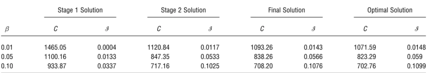
Table 1 Algorithm Output for the Calibration Problem b Stage 1 Solution C _I Stage 2 Solution C _I Final Solution C _I Optimal Solution C _I 0.01 1465.05 0.0004 1120.84 0.0117 1093.26 0.0143 1071.59 0.0148 0.05 1100.16 0.0133 847.35 0.0533 838.26 0.0566 823.29 0.059 0.10 933.87 0.0337 717.16 0.1025 708.20 0.1076 702.76 0.1099

uminÅarg min{C(un un): J(un)°bu, nÅ1, . . . , T}. (23) We set the unit cost uÅ2, the holding cost hÅ1, and the setup cost K Å 36 in all our test cases (including calibration). Results for other values of K and h, while not reported here, exhibited similar behavior to the ex-periments described here. In general, T is a stopping time that is a function of the stopping condition chosen for the algorithm. Here, we just choose a fixed number of iterations, TÅ50, in order to study the improvement of the algorithm. Improved performance in actual im-plementation can be achieved by a judicious choice of this condition. Each iteration consists of a simulation run of 20,000 periods, as this was sufficient to achieve steady-state conditions.

The true cost (

C

) and service level (

J

) of the Stage 1, Stage 2, and final solutions were estimated by perfor-mance evaluation of the inventory system at each so-lution point, using 30,000 periods and averaging over 10 replications. The additional periods and replications were chosen for further precision in the estimates, since they were used to determine ‘‘true’’ costs and solutions. The ‘‘true’’ optimal solutions were estimated by brute-force simulation over the (s, S) plane, initially using a 5 15 grid, and then searching over a 1 11 grid in the neighborhood of the coarse solution. Eachuon the grid was evaluated via ten 20,000 period replications, and the optimal solutionu* was estimated as

u*Åarg min{u

C

(u):

J

(u)°b*,u√Q}, (24) whereQrepresents the search space, andb* is an ap-propriately chosen ‘‘feasibility limit.’’ In particular, we setb* so that

J

(u*) É

_J

(umin), which then allows a fair comparison of the associated solution costs.

To measure the quality of our final solutions, we con-sidered the gap in the cost function

C

(u*)0

C

(u) rather than in the parameter value u* 0 u. Henceforth, the

word ‘‘precision’’ will denote the standard error of the concerned estimator. In terms of simulation, this will depend on the number of replications and the length of each run.

We calibrated the algorithm using exponentially dis-tributed demands, Poisson lead times with means of 100 and 6, respectively, and b Å0.01. This choice reflects our recommendation that the calibration problem be carried out on a case reflecting high lead time variability relative to the likely scenarios to be considered. The fea-sibility limit (b*) to generate the ‘‘true’’ optimal solution was set to be 0.015. Based on this calibration exercise, we fixed as(a0)Å2.25 and aQ(a0)Å0.15. Also, the values of s0(a0) and Q0(a0) were determined via this exercise to be 1435 and 85, respectively. We next carried out op-timizations of the same problem instance using service levels of 0.10 and 0.05. In these cases, the step sizes were determined using (20), (21), and (22), and the optimal solutions were generated using feasibility limits of 0.11 and 0.06, respectively. The results of this calibration are shown in Table 1.

The optimality gaps defined by (

C

0

_C

*)/

C

*, the CPU times (in seconds on a Sun Sparc10 workstation), and the fraction of total orders that arrive before previously placed orders (denoted as Cross Ratio, CR), are shown in Table 2.

The above results are quite representative of the large number of test cases that we considered. As can be seen, the final solution comes very close to optimality, and furthermore, the gap decreases with increasingb. The results also indicate that the Stage 2 solution given by the line search does well and is computationally very efficient. The order noncrossing assumption is grossly violated here, and consequently the Stage 1 solution (given by the analytic model of Tijms and Groenevelt) performs poorly. We also experimented with larger step

Table 2 Solution Quality for the Calibration Problem b Stage 1 Solution Gap (%) CPU CR (%) Stage 2 Solution Gap (%) CPU CR (%) Final Solution Gap (%) CPU CR (%) 0.01 36.72 É0 33.80 4.60 5.25 33.81 2.02 229.87 34.60 0.05 33.63 É0 33.80 2.92 5.25 33.81 1.81 229.93 34.80 0.10 24.75 É0 33.80 2.05 6.70 33.81 0.08 229.48 34.70

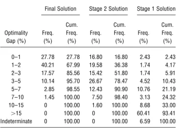
Table 3 Summary of Solution Quality for 1440 Problem Instances

Optimality Gap (%) Final Solution Freq. (%) Cum. Freq. (%) Stage 2 Solution Freq. (%) Cum. Freq. (%) Stage 1 Solution Freq. (%) Cum. Freq. (%) 0–1 27.78 27.78 16.80 16.80 2.43 2.43 1–2 40.21 67.99 19.58 36.38 1.74 4.17 2–3 17.57 85.56 15.42 51.80 1.74 5.91 3–5 10.14 95.70 26.67 78.47 4.52 10.43 5–7 2.85 98.55 12.43 90.90 10.76 21.19 7–10 1.45 100.00 7.50 98.40 3.13 24.32 10–15 0 100.00 1.60 100.00 8.68 33.00 ú15 0 100.00 0 100.00 60.41 93.41 Indeterminate 0 100.00 0 100.00 6.59 100.00

Table 4 Observed Service Levels of Final Solutions for 1440 Test Cases Target Service LT1 and LT2 Observed Service Number of Cases LT3 and LT4 Observed Service Number of Cases bÅ0.10 °0.105 236 °0.11 230 0.105–0.109 4 0.1100–0.1105 8 0.1105–0.1108 2 b*Å0.105 b*Å0.11 bÅ0.05 °0.055 239 °0.06 239 0.055–0.057 1 0.0600–0.0605 1 b*Å0.055 b*Å0.06 bÅ0.01 °0.0125 212 °0.0150 220 0.0125–0.0130 24 0.0150–0.0155 17 0.0130–0.0135 4 0.0155–0.0160 3 b*Å0.0125 b*Å0.015

sizes, and we observed a trade-off between the opti-mality gap and the true service level of the final solu-tion. Specifically, as the step size is increased, the opti-mality gap in general reduces, but the probability of the true service level exceeding feasibility limits is also in-creased. For instance, in the calibration case described above, as we increased asand aQfrom 2.25 and 0.15 to

4.50 and 0.75, respectively, the solution forbÅ0.01 im-proved significantly, but the corresponding solution for

bÅ0.10 had a true service level higher than 0.11. The numerical results for the 1440 problem instances are summarized in Table 3. The true service levels for these solutions, and the corresponding feasibility limits used to generate optimal solutions, are summarized in Table 4. For the Stage 1 solutions, the class ‘‘indeter-minate’’ indicates service levels that, though not grossly infeasible, significantly exceeded the feasibility limits and hence were incomparable with the generated opti-mal solutions.

The results indicate the following:

• The Stage 1 solutions have optimality gaps of over 15% for 60% of the cases; a further breakdown (not in-dicated in the results reported here) reveals that solu-tions for the low order-crossing LT1 cases (comprising 25% of the total instances) are within 10% of optimality, and as the extent of order crossing increases, so does the optimality gap.

• The Stage 2 solutions performed very well for the problem instances considered, with optimality gaps of under 5% in almost 80% of the cases.

• The optimization step significantly improves on the Stage 2 solution, with optimality gaps of under 5% in 95% of the cases.

• There is some degradation of solution quality asb

The results also clearly indicate that the vast majority of our solutions have service levels of no more than b

/0.01. The few cases that exceed this limit do so by a negligible amount. Further reductions (i.e., improve-ments) in service levels of the solutions (i.e., lower val-ues of b) can be achieved by suitably decreasing the value ofbu. The results shown in Table 4 also justify the

feasibility limits used for generating the optimal solu-tions.

6. Conclusions

In this paper, we have used gradient-based simulation optimization methods to address the problem of opti-mizing periodic review (s, S) systems that allow order crossings and are subject to a service level constraint. Simulation experiments show that currently available analytic models perform poorly under these conditions. We propose a simulation-based algorithm using the fea-sible directions approach from nonlinear programming. The implementation includes various preprocessing steps that generate good starting solutions. The algo-rithm is generally applicable to any problem having a single ‘‘noisy’’ constraint, with only the gradient esti-mation problem being system dependent.

The numerical results indicated the following: 1. Currently available analytic approximations would not be useful for managing (s, S) inventory sys-tems that are subject to even moderately high probabil-ities (such as that associated with LT2) of order cross-ings.

2. The proposed algorithm performed very well, us-ing a sus-ingle calibration over the entire set of test cases. The calibration provides benchmark settings on which parameter settings for a problem instance are easily scaled via Equations (20), (21), and (22). This robust-ness is attractive for practical implementation.

3. The Stage 2 preprocessing step provided impres-sive improvement at a relatively cheap cost in terms of computation. Although the optimization step usually reduces the gap of the Stage 2 solution by at least 50%, it is computationally much more intensive; the time for one optimization run ranges from one minute for LT1 to six minutes for LT4. A practitioner might consider terminating the procedure at Stage 2 for certain classes of products, e.g., those deemed less critical through Pa-reto analysis.

The algorithm performed very well over a large num-ber of test cases, and, in fact, the preprocessing step, by itself, yielded reasonable solutions within very short computing times. These promising computational re-sults motivate the need for further research on the al-gorithm’s theoretical properties. In addition, the need for a good stopping rule in practical implementation is an important topic for investigation. Lastly, extending the proposed algorithm to problems with multiple noisy constraints is also a fruitful topic for further in-vestigation.1

1_{M. C. Fu was supported in part by the National Science Foundation}

under Grant No. NSF EEC-9402384 and by a 1997 Summer Research Grant from the Maryland Business School. The authors sincerely thank the two anonymous referees for their constructive comments and sug-gestions that have led to a much improved paper.

References

Bashyam, S., M. C. Fu. 1994. Application of perturbation analysis to a class of periodic review (s, S) inventory systems. Naval Res.

Lo-gistics 41 47–80.

Ehrhardt, R. 1984. (s, S) policies for a dynamic inventory model with stochastic lead times. Oper. Res. 32 1 121–132.

Fu, M. C. 1994a. Sample path derivatives for (s, S) inventory systems.

Oper. Res., 42 351–364.

. 1994b. Optimization via simulation: A review. Ann. Oper. Res. 53 199–248.

. J. Q. Hu. 1994. (s, S) inventory systems with random lead times: Harris recurrence and its implications in sensitivity analysis.

Prob-ability Engng. Inform. Sci. 8 355–376.

, . 1997. Conditional Monte Carlo: Gradient Estimation

and Optimization Applications. Kluwer Academic Publishers,

Boston, MA.

Glasserman, P. 1991. Gradient Estimation Via Perturbation Analysis. Klu-wer Academic Publishers, Boston, MA.

Ho, Y. C., X. R. Cao. 1991. Discrete Event Dynamic Systems and

Perturbation Analysis. Kluwer Academic Publishers, Boston,

MA.

Jacobson, S. H., L. W. Schruben. 1989. A review of techniques for simulation optimization. Oper. Res. Letters 8 1–9.

Kushner, H. J., D. C. Clark. 1978. Stochastic Approximation Methods for

Constrained and Unconstrained Systems. Springer-Verlag, New

York.

L’Ecuyer, P., N. Giroux, P. W. Glynn. 1994. Stochastic optimization by simulation: numerical experiments with a simple queue in steady-state. Management Sci. 40 1245–1261.

Lee, H. L., S. Nahmias. 1993. Single-product, single-location models. S. C. Graves, A. H. G. Rinnooy Kan, P. H. Zipkin Eds. Handbooks

in Operations Research and Management Science, Vol. 4: Logistics of Production and Inventory, North-Holland, NY.

Luenberger, D. G. 1973. Introduction to Linear and Nonlinear

Program-ming, Addison-Wesley, Reading, MA.

Porteus, E. L. 1988. Stochastic inventory theory. D. Heyman, M. Sobel Eds. Handbooks in Operations Research and Management Science, Vol.

II: Stochastic Models, North-Holland, NY.

Safizadeh, M. H. 1990. Optimization in simulation: current issues and the future outlook. Naval Res. Logistics 37 807–825.

Schneider, H., J. L. Ringuest. 1990. Power approximation for computing (s, S) policies using service level. Management Sci. 36 7 822–834.

Tijms, H. C., H. Groenevelt. 1984. Simple approximations for the reorder point in periodic and continuous review (s, S) inventory systems with service level constraints. European J. Oper. Res. 17 175–190. Zheng, Y., A. Federgruen. 1991. Finding optimal (s, S) policies is about

as simple as evaluating a single policy. Oper. Res. 39 654–665. Zipkin, P. 1986. Stochastic lead times in continuous-time inventory

models. Naval Res. Logistics Quarterly 33 763–774.

Zoutendijk, G. 1960. Methods of Feasible Directions. Elsevier Publishing Company.