Surrogate-Assisted Evolutionary Deep Learning
Using an End-to-End Random Forest-based
Performance Predictor
Yanan Sun,
Member, IEEE,
Handing Wang,
Member, IEEE,
Bing Xue,
Member, IEEE,
Yaochu Jin,
Fellow, IEEE,
Gary G. Yen,
Fellow, IEEE,
and Mengjie Zhang,
Fellow, IEEE
Abstract—Convolutional neural networks (CNNs) have shown remarkable performance in various real-world applications. Un-fortunately, the promising performance of CNNs can be achieved only when their architectures are optimally constructed. The architectures of state-of-the-art CNNs are typically hand-crafted with extensive expertise in both CNNs and the investigated data, which consequently hampers the widespread adoption of CNNs for less experienced users. Evolutionary deep learning (EDL) is able to automatically design the best CNN architectures without much expertise. However, existing EDL algorithms generally evaluate the fitness of a new architecture by training from scratch, resulting in the prohibitive computational cost even operated on high-performance computers. In this paper, an end-to-end offline performance predictor based on the random forest is proposed to accelerate the fitness evaluation in EDL. The proposed performance predictor shows promising performance in term of the classification accuracy and the consumed compu-tational resources when compared with 18 state-of-the-art peer competitors by integrating it into an existing EDL algorithm as a case study. The proposed performance predictor is also compared with the other two representatives of existing performance predic-tors. The experimental results show the proposed performance predictor not only significantly speeds up the fitness evaluations, but also achieves the best prediction among the peer performance predictors.
Index Terms—evolutionary deep learning, performance pre-dictor, surrogate model, random forest, convolutional neural network.
I. INTRODUCTION
This work was supported in part by the National Natural Science Foundation of China under Grant 61803277, in part by the Fundamental Research Funds for the Central Universities, in part by the National Natural Science Fund of China for Distinguished Young Scholar under Grant 61625204, and in part by the Marsden Fund of New Zealand Government under Contracts VUW1209, VUW1509 and VUW1615, Huawei Industry Fund E2880/3663, and the University Research Fund at Victoria University of Wellington 209862/3580, and 213150/3662.
Y. Sun is with the College of Computer Science, Sichuan University, Chengdu 610065, China, and also with the School of Engineering and Computer Science, Victoria University of Wellington, Wellington 6140, New Zealand (e-mail: [email protected]).
B. Xue, and M. Zhang are with the School of Engineering and Computer Science, Victoria University of Wellington, PO Box 600, Wellington 6140, New Zealand (e-mails: [email protected]; and [email protected]).
H. Wang is with School of Artificial Intelligence, Xidian University, Xi’an 710071, China. (e-mail: [email protected]).
Y. Jin is with the Department of Computer Science, University of Surrey, Guildford GU2 7XH, U.K. (e-mail: [email protected]).
G. Yen is with the School of Electrical and Computer Engineering, Oklahoma State University, Stillwater, OK 74078 USA (e-mail:[email protected]).
H. Wang and B. Xue are the corresponding authors.
C
ONVOLUTIONAL Neural Networks (CNNs) [1], [2], as the most dominant deep learning approaches [3], have been demonstrating their promising performance in addressing various real-world applications, such as image classification [4], speech understanding [5], and natural language processing [6], to name a few. It is well known that the performance of CNNs highly relies upon their architectures, and a new architecture must be redesigned if the addressed data has been changed. Unfortunately, designing architecture with the best performance for the investigated data requires extensive expertise in both the CNNs and the data domain [7], which is not necessarily held by the interested users. Designing the best CNN architecture for the given data can be seen as an optimization problem, which can be mathematically formulated by (1):arg max
Aλ
L(Aλ,Dtrain,Dtest)s.t. λ∈Λ (1)
whereλrefers to the parameters related to the architectures of CNNs, such as the number of convolutional layers and the configurations of pooling layers; Λ refers to the parameter space,Aλdenotes the CNN algorithm Aadopting the
architec-ture parametersλ, andLmeans the performance measure ofAλ
on the test dataDtest after it has been trained on the training
data Dtrain. Generally, λ is with discrete values, e.g., the
configurations of both convolutional and pooling layers must be integers, which results in the architecture optimization not being well-addressed by the exact optimization algorithms. To address this challenge, researchers have developed algorithms (e.g., [8]– [14]) to design the best CNN architecture by effectively solving the problems represented in (1). Among these algorithms, the evolutionary algorithm-based ones, which are called the evolutionary deep learning algorithms (EDLs), are much preferred because EDLs generally consume less computational resource than other CNN architecture design algorithms [11]– [14], while still can achieve the promising results. For example, on the CIFAR10 dataset [15], the evolutionary algorithm-based Automatic Evolving CNN (AE-CNN) algorithm finds the best CNN architectures by consuming 22 days using three Graphics Processing Units (GPUs), and achieves the classification error rate of4.7%. However, the reinforcement learning-based neural architecture search method [9] consumes 28 days using 800 GPUs, while achieves the classification error rate of 6.01% which is a worse result than AE-CNN.
Evolutionary algorithm is a type of population-based heuris-tic computational paradigms [16]–[18], and has been widely used in addressing various complex optimization problems [19]– [21], mainly because of its gradient-free and insensitiveness to local minimum [22]–[24]. In EDLs, each individual is transformed to a CNN with the corresponding architecture through the mapping from genotype to phenotype, and then the weights of the CNN are initialized and iteratively trained based on Dtrain commonly with stochastic gradient descent
(SGD) [25], [26] given a number of epochs. During each epoch, the CNN also needs to be trained with multiple iterations in which the number is determined by the adopted batch size and the size of Dtrain. Such a single fitness evaluation
typically takes several hours to days. As a result, the potential promising architecture may not be found through EDLs within a limited computational budget due to the time-consuming fitness evaluation. This will become even more severe in the case of a large population and with a large number of generations, which is a more widely used configuration of evolutionary algorithms targeting at finding the better solutions [16], [18], [27]. Therefore, speeding up the fitness evaluation of CNN is essential in the design of EDL.
A common way to accelerate the fitness evaluation of CNN is to use a performance predictor [28]. In 2014, Swersky et al.
proposed the Freeze-thaw Bayesian optimization algorithm [29] by using a Gaussian process regression [16], which built the model based on the training performance in the firstt epochs to predict performance at theT (T > t) epoch. Followed by the same routine, the learning curve extrapolation methods in [30], [31] employed a set of functions from exponential families and the Bayesian neural network, respectively, to build the model based on the training performance in the first t epochs. Unfortunately, these mentioned performance predictors are typically based on expensive Markov chain Monte Carlo sampling procedures and manually designed curve functions, which are with high computational complexity. In 2017, Deng et al.proposed the Peephole algorithm [32] that predicted the performance of a CNN based on its architecture information, where a large number of different CNNs were trained, and the performance of all sampled networks in each epoch was collected as the training data, and then a long-short term memory neural network [33] is used to train the model. In addition, the train-less accuracy predictor (TAP) [34] and the accelerating neural network architecture search (ANNAS) [35] algorithms also employed similar methods to predict the performance of the given CNNs.
In fact, the optimization problem in EDLs is a type of computationally expensive problems, which is usually solved by surrogate-assisted evolutionary algorithms (SAEAs) [36], using cheap approximated regression and classification models (like Gaussian process model [37], radial basis function network [38], etc.) to replace the expensive fitness evaluation [39]. SAEAs have shown effectiveness and efficiency in various real-world optimization applications [40]. Generally, the models are trained from a small number of expensive fitness evaluations (i.e., the samples with evaluated objective values), and then the trained models are used as the fitness predictors in the evolutionary search to accelerate the optimization process [41].
According to [42], SAEAs can be divided into online and offline algorithms, which depend on whether expensive fitness evaluations are used to enrich the training data during the optimization process. Although new training data in online algorithms can significantly improve the quality of the model and optimization performance, offline algorithms are more practical than online algorithms due to the hardness and high cost in obtaining new data [40]. Without sampling new training data, offline algorithms can be very fast, and its data collection and optimization search are completely separated. So far, the base algorithms commonly applied in offline SAEAs are data pre-processing [43], data mining [42], and ensemble learning [44], since they can effectively and robustly address the problems having limited training data.
Our goal in this paper is to present an effective and efficient end-to-end performance predictor (in short named E2EPP) based on random forest [45]. The adoption of random forest remains in its effectiveness to a limited number of training samples, applicability to discrete variables, and robustness to its parameter settings [46], [47]. The proposed E2EPP is able to directly know the performance of a CNN once it looks at the new CNN architectures, which is naturally able to speed up the evolutionary process of EDLs. The contributions of this paper are summarized below:
1) The training data of the random forest are a set of data pairs, and each pair is composed of the CNN architecture and its performance. However, the architecture is modelled by describing languages, e.g., a paragraph of words, which cannot be directly used as the input to the random forest. Therefore, we propose an effective encoding method that is capable of extracting the features of CNN architectures as the numerical values, which are further used as the samples for training the random forest. As a case study, AE-CNN [48], as the representative of the state-of-the-art EDLs, is adopted to investigate the details of encoding. 2) The trained random forest is based on a set of samples
of CNN architectures (and their performance) which do not necessarily cover all the architecture space. If the performance prediction is adopted from the tree giving the best performance, the obtained result may be biased. To this end, we employ a selective ensemble strategy to choose diverse trees for combination in the local area of every generation.
3) Considering the two goals in term of using the per-formance predictor: the efficiency in speeding up the evolutionary process and the effectiveness in finding the best CNN architecture, we perform extensive experiments to verify these aspects.
The remainder of this paper is organized as follows. The background and related work are introduced in Section II. This is followed by the algorithm details of the proposed random forest-based performance predictor in Section III. In order to validate the effectiveness and the efficiency of the proposed performance predictor, the experiment designs and the experimental results are presented in Sections IV and V, respectively. Finally, the conclusion and future works are described in Section VI.
II. LITERATUREREVIEW
In this section, the EDL, AE-CNN and random forest are first introduced as the base algorithms in Subsection II-A, which is helpful to know the details of the proposed performance predictor. Then, the related work to performance predictors is presented in Subsection II-B, for better justifying the effectiveness and efficiency of the proposed work.
A. Background
1) EDL: A general framework of EDLs [11]–[14] is com-posed of the steps shown below:
Step 1: Randomly initialize a population with the predefined size based on the corresponding genotype-to-phenotype mapping strategy.
Step 2: Map each genotyped individual to the corresponding CNN, and train each CNN to obtain the classification accuracy on the validation dataset as its fitness value. Step 3: Use tournament selection to select the parent individ-uals based on the fitness, and then generate the new offspring achieving the same predefined size through the crossover and mutation operators.
Step 4: Perform the environmental selection on the combined population to select a new population surviving into the next generation.
Step 5: Go to step 3 if the termination condition is not satisfied. Otherwise, choose the individual with the best fitness and terminate the evolutionary process.
Indeed, the whole process of an EDL follows the procedure of an evolutionary algorithm, i.e., population initialization (Step 1), fitness evaluation (Step 2), offspring generation (Step 3) and environmental selection (Step 4). Generally, an evolutionary algorithm involves four parameters: the maximal generation number for the whole evolutionary process, the population size for the population initialization and the en-vironmental selection, and the crossover rate as well as the mutation rate for the offspring generation. One major factor of the promising performance of evolutionary algorithms is the environmental selection to keep individuals with better fitness in the new population than the previous population. However, as described in Step 2, the fitness of each individual in EDL is evaluated through the training of the corresponding CNN. For a better understanding of the fitness evaluation, the framework of training a CNN is provided in Algorithm 1.
Generally, the training of a CNN is achieved by using SGD on a given training dataset through hundreds of epochs (Steps 5-11). The objective of the training is to maximize the classification accuracy by adjusting millions of the weights (Step 8) in CNN. For a moderate CNN on a commonly used benchmark dataset, e.g., CIFAR10 and CIFAR100 [15], the training process would take from several hours to days perform-ing even on the high-performance GPUs. Since evolutionary algorithms belong to a class of population-based algorithms, their required numbers of evaluations are larger than that of SGD, which make the computational cost of EDL even higher. For example, on the CIFAR10 dataset, the large-scale evolutionary algorithm [12] consumed 11 days on 250 GPUs, and the hierarchical evolutionary algorithm [13] spent 1.5 days
Algorithm 1: Fitness Evaluation of A CNN in EDL
Input:The individualp, training dataset Dtrain,
validation dataset Dvalid, training epochs T,
batch sizeb, learning rateγ, objective function L.
Output: The fitness.
1 net← Decodepinto the corresponding CNN architecture;
2 Add the classification layer to the end of net; 3 Randomly initialize the weightswinnet; 4 t←0;
5 whilet < T do
6 foreach batch data inDtrain do
7 ∇w←Compute the gradient by∂L/∂w;
8 w←w−γ∇w;
9 end
10 t←t+ 1; 11 end
12 Calculate the classification accuracy ofnet onDvalid;
13 Return the fitness.
on 200 GPUs. Such a large number of GPUs may not be available to many researchers. To address such a challenge, it is of great importance to reduce the computational cost for EDLs by developing performance predictors, which could replace most of those expensive fitness evaluations, to speed up EDLs relying on limited computational resources.
2) AE-CNN: As the performance predictor is part of EDL in this research, an EDL method should be provided before the performance predictor is detailed. In this work, the AE-CNN algorithm developed by the authors is selected as the representative EDL, which is mainly based on the reasons that: 1) it shows promising performance among existing EDLs [48], and 2) the source code of AE-CNN is available to the public. Noting that the proposed performance predictor is applicable to any existing EDLs [8]–[14].
The AE-CNN algorithm [48] is an automatic EDL algo-rithm based on the building blocks of the state-of-the-art ResNet [49] and DenseNet [50], which has shown the promising performance on the CIFAR10 and CIFAR100 datasets [15] compared to state-of-the-art CNNs manually designed and other semi-automatic and automatic EDL algorithms [48]. The AE-CNN algorithm used in this work is to prepare samples for training the random forest, and then the trained random forest is used as the performance predictor in AE-CNN to verify the effectiveness and efficiency. In this subsection, we mainly introduce the genotype-to-phenotype mapping of AE-CNN for the completeness of the presentation, which enables the ability of evolutionary algorithms to model CNN architectures. These CNN architectures are the input to the random forest (the details of how to feed the architecture information to the random forest will be discussed in Section III).
The CNN architectures generated by AE-CNN are composed of the DenseNet Blocks (DBs), ResNet Blocks (RBs) and Pooling Blocks (PBs). Each DB or RB is composed of multiple DenseNet Units (DUs) and ResNet Units (RUs), respectively,
while a PB consists of only one pooling layer. Each DU, RU, or PB differs in terms of the parameter settings. The parameters of a DU are the sizes of input and output (denoted byin and
out, respectively), while those of an RU are the same as those of a DU, in addition to an increasing factor (denoted byk). The parameter of a PB is only the pooling type (i.e., the maximal
or meanpooling type) because its other parameters are all set to fixed values. Because a DB/RB is composed of multiple DUs/RUs, the parameters of a DB/RB are the corresponding parameters of a DU/RU and the amount (denoted byamount) of DUs/RUs in a DB/RB. In addition, as the DBs, RBs and PBs compose a CNN with an order, an extra parameter (denoted by
id) is also used to represent the corresponding position in the CNN. Obviously, a CNN generated by AE-CNN is composed of sequential blocks which may be the DUs, RUs or PBs. When the block is an RB, the parameters are theid,amount,inand
out; when the block is a DB, the parameters areid,amount,
k,inand out; when the block is a PB, the parameter is the pooling type denoted bytype. Noting that theinof the current RB/DB should be equal to theout of its previous RB/DB for the reason of constructing a valid CNN.
3) Random Forest: Compared with other learning algorithms, such as neural networks, the random forest has the advantages of directly accepting the discrete data as input, almost having no extra parameters to tune and not relying on a large amount of training data [50]. These advantages are the exact reason for employing the random forest in this work. Random forest [45] is an ensemble learning method by operating a set of decision trees for classification and regression tasks [46]. During the training of random forest, each decision tree randomly selects a part of the whole feature set and then learns the mapping from the selected features to the corresponding target. During the predicting process, each decision tree selects the same features as it selects in the training phase, and then output the corresponding prediction. The random forest uses the average output of the selected decision trees as its final output. Randomly selecting a part of the whole feature set is also the famous random subspace method [47], which has been shown to be simple yet effective.
B. Related Work
The existing performance predictors can be classified into two different categories: performance predictors based on the learning curve and end-to-end performance predictors, both of which are based on the training-predicting computational paradigm. The representatives of these two types are the Freeze-thaw Bayesian Optimization (FBO) algorithm [29] and the Peephole algorithm [32].
The FBO algorithm uses a regression model based on Bayesian Optimization to predict the performance of a CNN. The regression model is built based on the data sampled from the learning curve regarding the first t epochs, i.e., a series of data pairs in different training epochs and the corresponding performance at these epochs. After the regression model that has been optimized by the Bayesian Optimization method, it is used to predict the performance of the same CNN at the T-th epoch whereT > t. The Peephole algorithm uses a number of
CNN architectures and their corresponding performances that have been achieved by training the CNNs withT epochs, as the training samples to train a long-short time memory neural network [33]. The trained neural network directly predicts the performance of a new CNN based its architecture, which is called the end-to-end mechanism because the end in the input is the raw data while the end in the output is the classification accuracy. Because the architecture cannot be directly used as the input data of the neural network, the Peephole algorithm employs the word vector technique to map the CNN architecture to a numerical value.
The major advantage of the FBO algorithm remains in the trained-CNN-free nature, i.e., it does not need any trained CNNs in advance. Because training a CNN is time-consuming, varying from several days to weeks, the FBO algorithm is efficient. However, it will not be effective when the learning curve is not smooth because the curve fitting works under the assumption that the curve is smooth. In recent deep learning applications, the learning curve is usually not smooth because a schedule of learning rates is usually used. Once the learning rate is changed, the learning curve will have a non-smooth segment. Another limitation of the FBO algorithm is the non-end-to-end nature (i.e., in predicting the performance of each CNN, a part of the training data regarding this CNN must be collected for training the predictor), which requires much more labour work when it is used. Owing to the end-to-end nature, the Peephole algorithm is more convenient for use. However, the major drawback of Peephole remains in the requirement of a large number of training samples, which results in added computational complexity of collecting train samples exceeding the EDL without using performance predictors. For example, Peephole used over8,000 fully trained CNN architectures as the training data. However, EDLs generally achieve promising performance by evaluating only hundreds of individuals. If we have enough computational resources to evaluate the 8,000 CNN architectures, we will not need to develop the performance predictor. Such a limitation is largely caused by its adopted regression mode, i.e., the neural network-based algorithm, which typically highly relies on a large amount of labelled training data.
The proposed performance predictor has the advantages of the end-to-end manner and relying upon only limited training data, which address both limitations of the existing performance predictors discussed above.
III. PROPOSEDALGORITHM
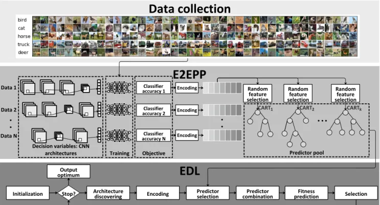
As mentioned, the main challenge of EDL is the high computational cost of evaluating a single CNN architecture. Inspired by offline SAEAs, we use random forest [46] as the fitness predictor to replace the expensive fitness evaluation. For a better understanding, Fig. 1 shows the framework of the proposed performance predictor as well as the associated EDL. The random forest-based performance predictor is learned from a number of different CNN architectures that have been trained for a classification task with their accuracy. Compared with the CNN training process, the random forest construction and prediction is computationally cheaper and can be repeatedly
Data collection
E2EPP
EDL
Data 1 Data 2 Data N Classifier accuracy 1 Classifier accuracy 2 Classifier accuracy NCART1 CART2 CARTk
Random feature selection Random feature selection Random feature selection
Initialization Architecture discovering Encoding Predictor selection combinationPredictor predictionFitness Selection
Encoding
Encoding
Encoding
Decision variables: CNN
architectures Training Objective Predictor pool
Stop? Output optimum
Fig. 1. Main frame of the proposed algorithm.
used throughout the evolutionary optimization. Thus, the high computational cost in EDL can be relieved.
As shown in Fig. 1 that is composed of three blocks, i.e., the data collection, E2EPP and EDL. The proposed E2EPP performance predictor is part of EDL. Firstly, a set of training data is collected for training the random forest-based predictor, where the collection is achieved by performing the corresponding EDL without using E2EPP. Each data sample is composed of the CNN architecture and the corresponding classification accuracy that is obtained by training the CNN from scratch. Secondly, those architectures are encoded into discrete code (shown in Subsection III-A) for building the random forest-based predictor pool with a large number (say
K) regression trees (denoted as CARTs) [51] (shown in Subsection III-B). During each generation of the EDL, the newly generated CNN architecture is encoded as the input to the random forest, and then its performance is predicted by using the adaptive combination of CARTs from the predictor pool (shown in Subsection III-C). When the EDL terminates, the CNN architecture that has the best prediction performance is output. Noting that there is no further CNN training during the optimization process.
Since the CNN architecture is presented as discrete variables, random forest [52], which is suited for discrete regression tasks and also relies on only limited labelled data [53], is adopted as the fitness predictor in the proposed algorithm. Also, as a selective ensemble of CARTs considering both global and local landscape, the random forest-based predictor is adaptively updated over the generations of the evolutionary search, where the population is distributed in different local regions and a fixed random forest cannot guarantee accuracy
in those local regions. In the following subsections, we will first introduce the details of encoding of the CNN architectures to the proper format for the random forest, training of the random forest, and fitness prediction using the trained random forest in Subsections III-A, III-B and III-C, respectively. Then, the strength and the weakness of the proposed performance predictor are summarized in Subsection III-D.
A. Encoding
The encoding operates on the trained CNNs whose architec-tures are randomly initialized. To collect this data, we use AE-CNN to randomly generate a set of valid AE-CNN architectures. A valid CNN architecture means that this architecture can be trained with a predefined training routine without any exceptions such as the out-of-memory errors causing a zero classification accuracy. Based on the description shown in Subsection II-A2, the collected training data are summarized as below:
1) RBs and DBs: Each generated CNN architecture is composed of four RBs and four DBs at most, the number of output channels of each block varies between[32,512] that is set based on the conventions of state-of-the-art CNNs [50], [54].
2) PBs: Each generated CNN architecture contains four pooling layers at most. There are two types of PBs: MAX and MEAN.
Generally, we encode a CNN architecture into a chromosome with3Nb+ 2Np discrete variables, when the maximal number
of RBs and DBs is Nb and the maximal number of PBs is
Algorithm 2: Encoding A CNN Architecture
Input:The CNN architectureA, the maximal number
Bn of DBs and RBs, the maximal numberNp
of PBs.
Output: The encoded architecture information. 1 b list← ∅;
2 p list← ∅;
3 l←Calculate the number of blocks inA; 4 forfor i←1 tol do
5 block←Get thei-th block ofA; 6 if block is a RBthen
7 Put 1into b list;
8 Put the values of theout andamount ofblock intob list;
9 else if block is a DBthen
10 Put the values of thek,outandamountof
blockinto b list;
11 else
12 if block is a maximal pooling layerthen 13 Put 1top list; 14 else 15 Put 0top list; 16 end 17 Put itop list; 18 end 19 end
20 Put zero tob list until|b list|= 3Nb; 21 Put zero top list until |p list|= 2Np; 22 Return b list∪p list.
into a triplet as [type,out,amount], where the block type for RBs is set to 1, and that for DBs are set to12,20and40 when k is equal to 12, 20and 40, respectively. Noting that the parameter ofinfor each RB/DB is not encoded because it can be calculated by the outof its previous RB/DB, and the smaller number of decision variables could result in a better performance for regression model when the training data is limited [46]. For the following 2Np variables, each pooling
layer is encoded into a pair as [pooling type, layer position], themaximalandmeanpooling types are presented by 1 and 0, respectively. If a CNN architecture has b RBs and DBs, and p PBs, then its3b+ 1-th to3Nb-th variables are set to
zeros, and its3Nb+ 2p+ 1-th to3Nb+ 2Np-th variables are
set to zeros as well. Therefore, the performance predictor by using random forest is based on the input data with3Nb+ 2Np
discrete decision variables, and the output is a continuous value within the range of [0,1]. Algorithm 2 shows the details of encoding a CNN architecture into the data that can be directly used by the random forest, and| · | is a countable operator.
B. Training of the Random Forest
A large number of CARTs are generated in the predictor pool. Each CART is trained by the whole training data with a random subset of features (i.e. discrete variables), where each discrete variable is assigned a probability of 0.5 in order to maximize the diversity of the predictor pool [55]. Each node
of a CART presents a rectangle region in the decision space. The mean squared error of the output of those samples in that region (node) determines whether this node needs splitting or not (i.e., whether the mean squared error decrease is smaller than a set thresholdTs[51], and if so, this node is a leaf node).
When K CARTs are obtained, the predictor pool is ready for the optimizer. The details of training the CARTs are shown in Algorithm 3.
Algorithm 3: Performance Predictor Training Input:TheK CARTs, the encoded training data
Dtrain, the feature numberm.
Output: TheK trained CARTs and their selected
feature ids. 1 I← ∅;
2 fori←1 toK do
3 CART ←Select the i-th CART from CARTs; 4 v∈Rm←Randomly generated a vector from
[0,1];
5 Ii ←Collect the position of the elements whose values are greater than 0.5 inv;
6 TrainCART on the features whose ids are in Ii; 7 I←I∪Ii;
8 end
Output: TheK trained CARTs and the corresponding
selected feature idsI.
C. Performance Prediction
Since the computational cost of training a single CNN is very high, it is impractical to obtain any new training data for the predictor pool during the optimization process. Thus, those predictors cannot be updated or validated, which is the main challenge of offline SAEAs [40]. To deal with the lack of training data, a large number of surrogate models are employed as ensemble members in a recent offline SAEA [44]. The results indicate that a selective ensemble surrogate can effectively improve the robustness of the obtained solution when the new training data is unavailable. Also, those ensemble members are adaptively combined in each generation to provide local information on the current population. Motivated by the combination strategy that was originally proposed in our previous work [44] for addressing decision variables having continuous values, we employ it to update the random forest-based predictor in every generation in the proposed algorithm, i.e., we choose QCARTs from the predictor pool and then use their average prediction as the fitness value. Although the decision variables of the proposed algorithm are discrete, it is experimentally found that the combination strategy still works well.
In each generation, all of theKtrained CARTs re-estimated the performance on the CNN Ab that has the best-predicted
fitness value; and thenQout of the K CARTs are uniformly selected from theK ordered CARTs based on their prediction values onAb. TheQCARTs are combined as the ensemble
performance predictor to evaluate both parent and offspring population. Such selection is based on the performance diversity
of CARTs around the current best CNN architecture Ab. After
that, the generated CNN architectures A are evaluated by using the ensemble predictor of QCARTs. Thus, the adaptive predictor can balance the global tendency and local information in the fitness landscape, where the combination of KCARTs predicts the global average landscape and that of Q diverse CARTs in a small area refines the local landscape. The details of the prediction process in a generation are shown in Algorithm 4.
D. Strength and Weakness of E2EPP
As have been introduced in Subsection II-B, the limitations of the existing performance predictors are the non-end-to-end nature, the strict assumption on the smoothness of the learning curve, and the availability of the large training samples. The proposed method has been carefully designed to address these limitations.
The proposed algorithm is end-to-end and does not rely on the learning curve no matter whether it is smooth or not. Firstly, the end-to-end nature is more convenient in practice because we do not need to prepare the training data in predicting the performance of each CNN. Secondly, because the proposed algorithm does not need to fit the learning curve, the predicted performance is better than the existing approaches based on the learning curve. This is theoretically evidenced by the universal approximation theorem [56] that the learning curve-based approaches can achieve promising performance only when the learning curve is smooth. However, in practice, the learning curve is not always smooth.
On the other hand, the proposed algorithm does not require a large number of training samples. Most existing approaches employing deep learning techniques succeed subject to the availability of a large amount of training data. In the CNN performance prediction, such training data is collected by training a lot of CNNs from scratch. However, the training is time-consuming even if performing on GPUs, while the main goal of designing performance predictors is to save the time of training CNNs. If we put enough time to collect a sufficient amount of training data, the performance predictor design will lose its original purpose. In the proposed method, we use the random forest as the base operator to learn the mapping between the CNN architecture and its performance. The reason is that random forest can achieve a promising performance on limited amount of training data, which has been theoretically proven and practically investigated [45], [46].
Unfortunately, the weakness of the proposed algorithm is the unknown of the minimal number of training samples for achieving promising performance, while the minimal number is case by case for different tasks. In practice, we need to use an incremental strategy to sample training samples until the desired performance is achieved.
IV. EXPERIMENTDESIGN
In order to verify the effectiveness and efficiency of the proposed performance predictor, a series of experiments are carefully designed and performed. Although the proposed performance predictor aims at speeding up the fitness evaluation of EDL, the ultimate goal of the performance predictor is
Algorithm 4: Performance Predicting
Input:TheK trained CARTs, the selected features ids
I of each CART, the current best CNNAb, the
number of most diverse predictionQ, the generated architecturesAto be evaluated. Output: The fitness values ofA.
1 Y ← ∅;
2 Abencoded←EncodeAb based on the details shown in Subsection III-A;
3 fori←1 toK do
4 CART ←Select the i-th CART from CARTs; 5 x←FromAbencoded select the elements whose ids
are in Ii;
6 y←UseCART predict the classification accuracy on x;
7 Y ←Y ∪x;
8 end
9 Y ←Order the elements inY;
10 IselectedCART ←Uniformly select QCARTs based onY; 11 fori←1 to|A|do
12 Fi←the mean prediction ofQselected CARTs
(ICART
selected) on|Ai|;
13 end 14 Return F.
to find the best CNN architecture that achieves a promising classification performance on the image data at hand. Therefore, two experiments are performed in this paper: 1) investigating the classification performance of the proposed performance predictor with AE-CNN, and 2) inspecting the efficiency of the proposed performance predictor. In this section, the selected peer competitors and benchmark datasets, as well as the parameter settings for these two types of experiments, are detailed.
A. Peer Competitors
In comparing the classification performance, the chosen peer competitors are divided into three different categories: the state-of-the-art CNNs whose architectures are manually designed, the state-of-the-art CNN architecture designs based on non-evolutionary algorithms (mainly based on reinforcement learning), and the state-of-the-art EDL algorithms. The first category covers DenseNet [50], ResNet [54], Maxout [57], VGG [58], Network in Network [59], Highway Network [60], All-CNN [61], FractaNet [62]. Considering the promising performance of ResNet, we use its two different versions: ResNet with the depths of 101 and 1,202, respectively. For the convenience of the discussion, they are denoted as ResNet (depth=101) and ResNet (depth=1,202), respectively. The second category consists of NAS [9], MetaQNN [8], EAS [9], and Block-QNN-S [10]. The third category includes Genetic CNN [11], Large-scale Evolution [12], Hierarchical Evolution [13], and CGP-CNN [14]. Considering the proposed performance predictor is introduced in a case study of AE-CNN, AE-CNN combined with E2EPP (denoted as AE-CNN+E2EPP) is chosen to perform this experiment.
bird
cat
horse
(a) CIFAR10baby
dolphin
snail
(b) CIFAR100Fig. 2. Examples of CIFAR10 and CIFAR100 shown in Figs. 2a and 2b, respectively. Each row represents two samples from the same category and the words in the left refer to the corresponding category name.
For the second experiment, the selected peer competitors are the existing performance predictors [30], [32] discussed in Subsection II-B.
B. Benchmark Datasets
Benchmark datasets are only required by the first experiment. The CIFAR10 and CIFAR100 datasets are selected as the benchmark datasets. Both benchmark datasets are selected mainly because of their wide adoption by the state-of-the-art CNNs and CNN architecture design algorithms.
CIFAR10 is a 10-category natural object classification dataset, consisting of a training dataset with 50,000 images and a test dataset with 10,000images, and each image has the dimension of 32×32. In the training dataset, each category has roughly the equal number of samples, while in the test dataset, each category has the exact same number of samples. CIFAR100 is just like CIFAR10, except that it is 100-category. Because CIFAR100 has the same number of images in the training images and test images as those of CIFAR10, each category in CIFAR100 only has one-tenth of images as that in CIFAR10. Due to the smaller number of training data in each category and a larger number of classification categories than CIFAR10, CIFAR100 is a more complex dataset for classification than CIFAR10.
For each image of both benchmark datasets, the object to be classified commonly occupies a small area of the entire image, and also the size, the area, and the position of each object differ to each other in other images, even when they are from the same category. An example of these two benchmark datasets are shown in Fig. 2 for a glance, where each row denotes the objects from the same category, and the label leading in each row denotes the ground-truth of the corresponding object.
C. Parameter Settings
In this subsection, the parameter settings for generating the training data from AE-CNN are detailed at first, and then those of the proposed performance predictor are introduced next. Noting that these parameter settings are applied to both experiments.
Based on the conventions of the deep learning community, the SGD algorithm is used to train the CNN architectures whose weights are initialized with the commonly used Xavier method [63]; the batch size is set to 128; the weight decay is set to 5×10⁻⁴; each CNN is trained 350 epochs, and the learning rate is set to 0.01 for the first epoch and the
151-th to the249-th epoch,0.1 for the second to the150-th epoch, and0.001 for the remaining epochs. The classification accuracy is evaluated on the “validation dataset1”. Because
the used benchmark datasets do not have the corresponding validation dataset,20%images are randomly selected from the corresponding training dataset as the validation dataset based on the conventions. All the CNNs are trained on three GPUs with the same model of NVIDIA 1080TI. In addition, we set both maximal numbers of RB and DB to 4 because of the limited GPU memory. Because each pooling operation halves the input size one time, and the input sizes of CIFAR10 and CIFAR100 are both32×32, the maximal number of pooling layers is set to 4. Furthermore, based on the conventions of DenseNet,k is selected from {12,20,40}, and the maximal numbers of DUs in a DB are10whenk= 12andk= 20, and 5 whenk= 40. The maximal number of RUs in an RB is set to10. Based on our configuration for generating the training data,Nb andNp are set equal to8and4, respectively, and the
decision variable length of each training data for the random forest is32(8×3 + 4×2). To build the performance predictor pool, we generate 1000 CARTs. The threshold of stopping node splitting is set as1e−4×σ2 (σ2is the variance of the
training data) when growing each CART. In each generation, 100 CARTs are selected to combine the random forest-based predictor.All the parameter settings are summarized in Table I.
In performing the CNN architecture design by using AE-CNN and the proposed E2EPP method, we set both the maximal generation number and the population size to 20, the probabilities for the crossover and mutation are set to 0.9 and 0.1, respectively, as suggested in AE-CNN. Noting that before E2EPP is used for each generated CNN architecture, the CNN architecture is evaluated in the GPUs for one epoch so that the generated CNN can be normally evaluated by E2EPP, i.e., the employed GPUs can carry the CNN architecture and will not lead to an out-of-memory error. This is also for keeping a similar data distribution between the training data and the test data for E2EPP. After the evolutionary process, the individual with the best classification accuracy is chosen and then fully trained with the same training routine as collecting
1We are aware of different definitions on the validation (data)set from
literature. Based on the convention of the machine learning community, the validation set is used only for controlling overfitting and model selection, and the selected model cannot be updated and improved via the validation set. In evolutionary deep learning, after the individuals (models) are selected based on their performance of the “validation set”, they are updated and possibly improved by genetic operators during evolution. So we use the quotation marks to highlight its different meaning here from its traditional meaning.
the training data for five independent runs, and the best result is reported, which is followed the conventions from deep learning community.
TABLE I
ASUMMARY OF THE PARAMETER SETTINGS. Parameter name Parameter value
batch size 128
weight decay 5×10⁻⁴
training epochs 350
learning rate 0.01for1, and151–249epochs; 0.1 for 2–150 epochs;0.001 for 251–350epochs
kof the DB {12,20,40}
maximal number of DUs in a DB 10whenk= 12andk= 20;5 whenk= 40
maximal number of RUs in a RB 10 maximal number of DBs (Np) 4 maximal number of RBs (Nb) 8 generation number 20 population size 20 crossover probability 0.9 mutation probability 0.1 number of CARTs 1000
threshold of stopping node splitting 1e−4×ρ2 (ρ2is the variance of the training data)
number of selected CARTs 100
V. EXPERIMENTALRESULTS
The results of the designed experiments are presented and analyzed in this section. Specifically, the classification performance of AE-CNN+E2EPP, in terms of the classification accuracy and the consumed GPU days, are elaborated in Subsection V-A. In order to extensively investigate the proposed E2EPP performance predictor, its efficiency and effectiveness are individually tested, and the corresponding experimental results are shown in Subsections V-B and V-C, respectively. In addition, the comparision to Radial Basis Network (RBN) has also been done to show the promising performnace of random forest employed in the proposed E2EPP performance predictor.
A. Overall Results
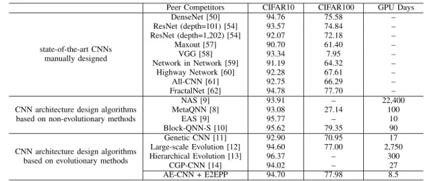
Table II presents the experimental results in terms of the classification accuracy and consumed GPU days of the com-pared algorithms. Specifically, Table II is divided into five rows: the second to fourth rows denote the state-of-the-art CNNs manually designed, the state-of-the-art CNN architecture design algorithms based on non-evolutionary algorithms, and the state-of-the-art CNN architecture design algorithms based on evolutionary algorithms (i.e., the EDL algorithms), respectively; the last row shows the result of the proposed performance predictor used in AE-CNN (i.e., AE-CNN+E2EPP). In addition, the first column shows the names of the compared algorithms; the second and the third columns show the classification accuracy on CIFAR10 and CIFAR100, and the fourth column shows the consumed GPU days for achieving the corresponding classification accuracy by the corresponding architecture design algorithms. These architecture design algorithms generally report their consumed numbers of GPUs and days. For the convenience of the comparison, we unify them by using “GPU
days” as an indicator expressing the utilized computational resource. For example, one GPU day means a GPU is fully consumed in one day to achieve the classification accuracy. All the results of the peer competitors in this table are extracted from their seminal papers, in addition to the GPU days that we convert it by multiplying the number of GPUs with the number of days taken. The symbol “–” means the corresponding paper does not provide the corresponding result publicly available. Noting that the GPU days of AE-CNN+E2EPP is mainly caused by collecting the training data but not performing E2EPP.
For the classification accuracy obtained by the state-of-the-art CNN manually designed, on the CIFAR10 benchmark dataset, AE-CNN+E2EPP achieves, on the average, the classification accuracy of 1.5% higher than ResNet (depth=101), VGG and All-CNN,2.04%higher than ResNet (depth=1,202) and Highway Network, and even3.78% higher than Maxout and Network in Network, respectively, while slightly lower than DesnNet (0.04%) and FractalNet (0.06%). On the CIFAR100 benchmark dataset, AE-CNN+E2EPP, whose classification accuracy is77.98%, outperforms all other peer competitors that achieve the classification accuracy varying from77.70% (by FractalNet) to61.40% (by Maxout). AE-CNN+E2EPP demon-strates the promising performance among peer competitors in this category.
Compared with non-evolutionary algorithms, AE-CNN+E2EPP achieves the better classification accuracy than NAS and MetaQQ, but a little worse than EAS and Block-QNN-S on CIFAR10; on CIFAR100, the classification accuracy of AE-CNN+E2EPP is significantly better than that of MetaQQ while slightly worse than that of Block-QNN-S. In addition, NAS, MetaQNN and Block-QNN-S achieve their classification accuracies by consuming22,400,100 and 90 GPU days, respectively, while AE-CNN+E2EPP only consumes8.5GPU days. In addition, AE-CNN+E2EPP also consumes fewer GPU days than that of EAS.
Compared with other EDLs, AE-CNN+E2EPP shows lower classification accuracy than that of Hierarchical Evolution, while higher than those of Genetic CNN, Large-scale Evolution and CGP-CNN on CIFAR10. On CIFAR100, AE-CNN+E2EPP shows the highest classification accuracy than others. Further-more, AE-CNN+E2EPP also consumes the fewest GPU days than other peer competitors in this category.
In fact, EAS, Block-QNN-S, Hierarchical Evolution and CGP-CNN are all semi-automatic CNN architecture design al-gorithms, i.e., they design the CNN architectures based on both the expertise of manually designed CNNs and the automatic ways of EDLs. To this end, it is reasonable that CNN+E2EPP is inferior to them in terms of the classification accuracy. In summary, AE-CNN+E2EPP wins 26 times out of the 30 classification accuracy comparisons, and also consumes the least GPU days among all architecture design peer competitors.
B. Efficiency of E2EPP
The experimental results presented in Table II have indicated that AE-CNN can achieve promising classification accuracy when the proposed E2EPP is used, which is the ultimate goal of designing the performance predictor. In this subsection,
TABLE II
THE COMPARISON OFAE-CNN+E2EPPAND THE PEER COMPETITORS IN TERMS OF THE CLASSIFICATION ACCURACY(%)AND THE CONSUMEDGPU DAYS ON THECIFAR10ANDCIFAR100BENCHMARK DATASETS.
Peer Competitors CIFAR10 CIFAR100 GPU Days
state-of-the-art CNNs manually designed DenseNet [50] 94.76 75.58 – ResNet (depth=101) [54] 93.57 74.84 – ResNet (depth=1,202) [54] 92.07 72.18 – Maxout [57] 90.70 61.40 – VGG [58] 93.34 7.95 – Network in Network [59] 91.19 64.32 – Highway Network [60] 92.28 67.61 – All-CNN [61] 92.75 66.29 – FractalNet [62] 94.78 77.70 –
CNN architecture design algorithms based on non-evolutionary methods
NAS [9] 93.91 – 22,400
MetaQNN [8] 93.08 27.14 100
EAS [9] 95.77 – 10
Block-QNN-S [10] 95.62 79.35 90
CNN architecture design algorithms based on evolutionary methods
Genetic CNN [11] 92.90 70.95 17
Large-scale Evolution [12] 94.60 77.00 2,750
Hierarchical Evolution [13] 96.37 – 300
CGP-CNN [14] 94.02 – 27
AE-CNN + E2EPP 94.70 77.98 8.5
we will specifically investigate the efficiency of E2EPP by disabling and enabling it in AE-CNN. To do a fair comparison, AE-CNN is performed with the same parameter settings as those of AE-CNN+E2EPP on both CIFAR10 and CIFAR100. We record the consumed GPU days of AE-CNN when it has a new generated CNN architecture whose fitness value satisfies the condition formulated by (2)
f1−f2 f2 ≤0.01 (2)
where f1 denotes the fitness of the new CNN architecture
generated by AE-CNN, and f2 denotes the fitness of
AE-CNN+E2EPP shown in Table II.
CIFAR10
CIFAR100
0 5 10 15 20 25 30 35GPU days
7
22
10
33
AE-CNN+E2EPP AE-CNNFig. 3. The consumed GPU days of AE-CNN and AE-CNN+E2EPP when achieving the same classification accuracy on CIFAR10 and CIFAR100.
Fig. 3 shows the comparisons of the consumed GPU days when AE-CNN satisfies the condition of (2) on CIFAR10 and CIFAR100. The numbers above each bar display the consumed GPU days by the corresponding algorithm. The bars filled with the symbol of “·” denote the results of AE-CNN+E2EPP, while the bars filled with the symbol of “◦” denote that of AE-CNN. Clearly, it can be seen from Fig. 3 that E2EPP has significantly
improved the efficiency of AE-CNN for finding the best CNN architectures. Particularly, E2EPP saves214%and230%fewer GPU days on CIFAR10 and CIFAR100, respectively, when it is used in AE-CNN. Therefore, the goal of designing such a proposed performance predictor, in terms of speeding up the fitness evaluation, has been achieved.
C. Effectiveness of E2EPP
In order to check the effectiveness of E2EPP, the FBO [30] and Peephole [32] algorithms, which are the representatives of existing performance predictors as detailed in Subsection II-B, are selected to do the quantitative and qualitative comparisons against E2EPP. For the quantitative comparison, we choose the Mean Square Error (MSE), Kendall’s Tau (KTau) [64] and the Coefficient of Determination (CoD) [65] as the indicators suggested in [32]. Specifically, KTau measures the correlation between the ranks of the prediction and their true ranks. A higher KTau value implies the higher correlation and the KTau value varies between[−1,1]. The CoD measures the closeness degree of the prediction to its true value, and its value ranges from−∞to1 where a larger value means the closer degree. For the qualitative comparison, we scatter the true values with the corresponding prediction on a 2-dimension space where the horizontal axis denotes the true values while the vertical axis denotes the prediction. The parameter settings of FBO and Peephole are set based on the suggestions in [32]. In addition, the experiment on each benchmark dataset is performed 10 times.
TABLE III
THEMEANSQUAREERROR(MSE), KENDALL’STAU(KTAU), COEFFICIENT OFDETERMINATION(COD)AND THE USED TIME OFFBO,
PEEPHOLE,ANDE2EPPALGORITHMS ON THECIFAR10DATASET.
MSE KTau CoD Time (seconds)
FBO 0.0077 0.2170 -4.346 3.702
Peephole 0.0019 0.5324 0.3765 359.296 E2EPP 0.0006 0.6604 0.5184 3.813
0.70 0.75 0.80 0.85 0.90 0.95 1.00 0.70 0.75 0.80 0.85 0.90 0.95 1.00 (a) FBO 0.70 0.75 0.80 0.85 0.90 0.95 1.00 0.70 0.75 0.80 0.85 0.90 0.95 1.00 (b) Peephole 0.70 0.75 0.80 0.85 0.90 0.95 1.00 0.70 0.75 0.80 0.85 0.90 0.95 1.00 (c) E2EPP
Fig. 4. The prediction and the true values of EBO, Peephole and E2EPP on the CIFAR10 dataset. In each subfigure, the horizon axis denotes the true values, while the vertical axis denotes the corresponding prediction.
0.50 0.55 0.60 0.65 0.70 0.75 0.80 0.50 0.55 0.60 0.65 0.70 0.75 0.80 (a) FBO 0.50 0.55 0.60 0.65 0.70 0.75 0.80 0.50 0.55 0.60 0.65 0.70 0.75 0.80 (b) Peephole 0.50 0.55 0.60 0.65 0.70 0.75 0.80 0.50 0.55 0.60 0.65 0.70 0.75 0.80 (c) E2EPP
Fig. 5. The prediction and the true values of EBO, Peephole and E2EPP on the CIFAR100 dataset. In each subfigure, the horizon axis denotes the true values, while the vertical axis denotes the corresponding prediction.
TABLE IV
THEMEANSQUAREERROR(MSE), KENDALL’STAU(KTAU), COEFFICIENT OFDETERMINATION(COD)AND THE USED TIME OFFBO,
PEEPHOLE,ANDE2EPPALGORITHMS ON THECIFAR100DATASET.
MSE KTau CoD Time (seconds)
FBO 0.0078 0.1923 -2.631 3.725
Peephole 0.0024 0.5412 0.3238 458.652 E2EPP 0.0015 0.6501 0.3872 3.514
The quantitative comparison results on CIFAR10 and CI-FAR100 are shown in Tables III and IV, respectively. In addition, we also add the consumed time (seconds) measuring how long E2EPP, FBO and Peephole take to finish the experiment. Clearly as can be seen from Table III, FBO and Peephole obtain the MSE of 0.0077, and 0.0019, respectively, while E2EPP obtains the MSE of 0.0006 that is an order of magnitude less than FBO and Peephole can. This means that E2EPP could achieve a better prediction than FBO and Peephole. For the KTau indicator, FBO, Peephole and E2EPP achieve the values of 0.2170, 0.5324 and 0.6604, respectively, which imply that the performance predicted by E2EPP has the best correlation. For the CoD indicator, E2EPP again wins the highest value of 0.5184 (-4.346 for FBO and 0.3765 for Peephole). Based on the definition of CoD, the predicted value of E2EPP is the closest one to the ground truth value among the comparisons. In addition, E2EPP uses 3.813 seconds for the prediction, which is a little worse than FBO that uses 3.702 seconds. However, it is still much better than Peephole that
uses 359.296 seconds. The similar comparison results can also be investigated from Table IV. Specifically, E2EPP obtains the MSE of 0.0015 that is about half of that from Peephole and 1/5 of that from FBO, i.e., E2EPP has the minimal prediction error than the others. Furthermore, FBO obtains the KTau indicator value of 0.1923, while Peephole and E2EPP obtain the values of 0.5412 and 0.6501, respectively. For the CoD indicator, E2EPP achieves the best one, i.e., 0.3872, while FBO and Peephole acquire -2.631 and 0.3238, respectively. This shows the best prediction performance of E2EPP on the CIFAR100 dataset. In addition, E2EPP consumes 3.514 seconds to finish the prediction, which is the best among FBO (3.725 seconds) and Peephole (458.652 seconds).
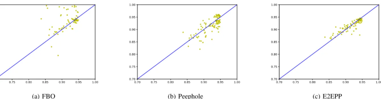
The qualitative comparisons on CIFAR10 and CIFAR100 are scattered in Figs. 4 and 5, respectively, where thexaxis of each point (denoted as(x, y)) represents the true value andy
axis denotes the corresponding prediction. For the convenience of the comparison, we also plot the liney=xin each figure. The points standing above y = x mean the predictions are higher than the true values, while the points standing below
y =xmeans the predictions are lower than the true values. The more points closer toy=x, the better prediction of the corresponding performance predictor. As can be clearly seen from Figs. 4a and 4b, FBO has only half of the total points that are close to the line of y = x, and Peephole achieves better results by having more points close to the line ofy=x. However, it is clearly observed from Fig. 4c showing the results of E2EPP, almost all of the points are close to the liney=x.
This means that the predicted values of E2EPP have minimal prediction errors, which is consistent with the quantitative analysis shown in Table III. From Figs. 5a, 5b and 5c that show the results performed on CIFAR100 by FBO, Peephole and E2EPP, respectively, it can be seen that FBO and Peephole achieve the similar results that have a wide spread of points around the line of y=x, while the results of E2EPP have the closer distance to the line y =x. This also shows the same conclusion from the quantitative analysis observed in Table IV.
D. Comparison to Radial Basis Network (RBN)
In order to demonstrate the promising performance of the random forest employed by the proposed E2EPP performance predictor, the comparison to RBN is performed, and the results are shown and analyzed in this subsection.
Specifically, an RBN is a three-layer neural network, except that the activation function of each unit in the hidden layer is a Gaussian function, and the output layer is a linear weight summation of the output of the hidden layer. The RBN is often used for regression tasks, which is similar to the function of random forest used in the proposed E2EPP performance predictor. Another reason for choosing RBN here for the comparison is that RBN is the base of our previous work [44] that motivates the design of E2EPP in this paper. For a fair comparison, we only replace the random forest by an RBN, while the other parts are kept the same as that used for the experiment shown in Subsection V-A. For the convenience of the discussions, we denote the RBN used by the AE-CNN algorithm as AE-CNN+RBN.
In the comparison, we only show the classification accuracies on CIFAR10 and CIFAR100, but not showing the consumed GPU days since the performance of both AE-CNN+E2EPP and AE-CNN+RBN does not rely on GPUs. The number of GPU days shown in Table II of AE-CNN+E2EPP is used for measuring the validity of the generated CNN architectures during the evolutionary process. In addition, the number of hidden units of the RBN is set to the same as the input size based on the conventions of practice [44]. The comparison results are shown in Table V.
TABLE V
THE COMPARISON OFAE-CNN+E2EPPANDAE-CNN+RBNIN TERMS OF THE CLASSIFICATION ACCURACY(%)ON THECIFAR10ANDCIFAR100
BENCHMARK DATASETS.
CIFAR10 CIFAR100
AE-CNN + E2EPP 94.70 77.98
AE-CNN + RBN 82.33 70.20
It can be seen from Table V that AE-CNN+E2EPP achieves the classification accuracies of 94.70% and 77.98% on CI-FAR10 and CICI-FAR100, respectively, while AE-CNN+RBN achieves those of 82.33% and 70.20%, respectively. This implies that the random forest employed in the proposed E2EPP performance predictor is better than RBN. In fact, it is easy to find the proof of this conclusion, when the RBN is used, the mean and standard deviations of the Gaussian functions are calculated based on the training data. However, the training data in E2EPP is encoded with some numerical
numbers that do not refer to the real meaning. In addition, the RBN has been well-known to be suitable for continuous data, while the training data in E2EPP is discrete. In summary, AE-CNN+E2EPP outperforms AE-CNN+RBN on the CIFAR10 and CIFAR100 benchmark datasets.
As can be seen above, we have performed four groups of experiments that are carefully designed to verify the promising performance of the proposed E2EPP performance predictor. Particularly, the first is for investigating whether E2EPP could enable EDL to achieve the competitive performance in designing the CNN architectures. The second validates whether E2EPP could accelerate EDL or not. The third quantitatively and qualitatively investigates whether E2EPP could outperform the existing approaches regarding the performance prediction, and the fourth investigates whether the random forest employed in E2EPP could perform better than the RBN that is another commonly used regression model. In addition to the third one, all the others are performed in the case of AE-CNN. All the experimental results demonstrate the effectiveness and efficiency of the proposed E2EPP performance predictor. From these experimental results, we can recognize that the performance predictor is indeed able to speed up EDL, and the end-to-end nature is convenient to use in practice by avoiding manual interventions during the performing of EDL. In addition, the random forest, as an ensemble approach, achieves the promising performance but relying on only limited training samples, which is a good characteristic especially in EDL where sufficient training data is not easy to obtain. Furthermore, the random forest could directly use the discrete number as its input, which is also another good characteristic in predicting the performance of CNNs when the architecture information is used as the input data. This implies that the ensemble methods depend on discrete input data may be a proper choice in designing the performance predictors, which is not only suitable to EDL but also other deep learning model selection methods.
VI. CONCLUSIONS ANDFUTUREWORK
The goal of this paper was to develop an effective and efficient end-to-end performance predictor, named E2EPP, to speed up evolutionary deep learning algorithms in designing the best CNN architectures for given tasks. This goal has been achieved by proposing a random forest-based offline surrogate model. In order to enable the random forest to accept the CNN architectures as its input data, we also develop an encoding schema that is able to uniquely map the description of a CNN architecture into a numerical decision variable. In addition, we took the advantage of random forest in terms of the ensemble characteristic that each tree in the random forest randomly selects a subspace of the whole features as its training data. Furthermore, in order to improve the diversity of used off-line model, only a part of the decision trees in the random forest is selected based on their prediction on the best individual to do the prediction, which in turn enhances the accuracy of the predicted values. The proposed performance predictor is firstly examined by integrating it into an existing evolutionary deep learning algorithm, which is called AE-CNN+E2EPP, on CIFAR10 and CIFAR100. Through
the comparisons with eight CNNs whose architecture are manually crafted, and another eight CNN architecture designs, AE-CNN+E2EPP shows the very promising results on both classification accuracy and consumed GPU days. In addition, the efficiency of the E2EPP is also examined on AE-CNN by enabling and disabling it. The results show that E2EPP could save 2/3 of computational time when achieving the same classification accuracy. Further, the E2EPP is compared with the other two state-of-the-art performance predictors, namely FBO and Peephole, on three measurements. E2EPP shows the best results on these three measurements. Especially, E2EPP uses only 1/100 computational time of that Peephole uses. It also shows that E2EPP achieves the best prediction through the qualitative comparison among these three performance predictors on both CIFAR10 and CIFAR100 datasets.
The proposed performance predictor is based on the first-train-then-to-predict paradigm, which requires a set of trained samples in advance. Theoretically, the more trained samples, the better prediction results. However, collecting more trained samples implies consuming more computational resource, which leads to long processing time. Achieving a better performance prediction results conflicts to the goal of designing the performance predictors. Therefore, finding a good balance between these two objectives may be an efficient way to use the performance predictor, which is left for future work. In addition, we will also integrate E2EPP into other CNN architecture design algorithms to solve some specific tasks, such as recognizing breast cancer on the BreakHis dataset [66].
REFERENCES
[1] A. Krizhevsky, I. Sutskever, and G. E. Hinton, “Imagenet classification with deep convolutional neural networks,” in Advances in Neural Information Processing Systems 25, Lake Tahoe, Nevada, USA., 2012, pp. 1097–1105.
[2] Y. Leung, Y. Gao, and Z.-B. Xu, “Degree of population diversity-a perspective on premature convergence in genetic algorithms and its markov chain analysis,”IEEE Transactions on Neural Networks, vol. 8, no. 5, pp. 1165–1176, 1997.
[3] Y. LeCun, Y. Bengio, and G. Hinton, “Deep learning,”Nature, vol. 521, no. 7553, pp. 436–444, 2015.
[4] T. N. Sainath, A.-r. Mohamed, B. Kingsbury, and B. Ramabhadran, “Deep convolutional neural networks for LVCSR,” inProceeding of 2013 IEEE International Conference on Acoustics, Speech and Signal Processing. Vancouver, Canada: IEEE, 2013, pp. 8614–8618.
[5] O. Abdel-Hamid, A.-r. Mohamed, H. Jiang, L. Deng, G. Penn, and D. Yu, “Convolutional neural networks for speech recognition,” IEEE/ACM Transactions on Audio, Speech, and Language Processing, vol. 22, no. 10, pp. 1533–1545, 2014.
[6] I. Sutskever, O. Vinyals, and Q. V. Le, “Sequence to sequence learning with neural networks,” inAdvances in Neural Information Processing Systems 2014, Montreal, Canada, 2014, pp. 3104–3112.
[7] Y. Sun, G. G. Yen, and Z. Yi, “Evolving unsupervised deep neural networks for learning meaningful representations,”IEEE Transactions on Evolutionary Computation, vol. 23, no. 1, pp. 89–103, 2019. [8] B. Baker, O. Gupta, N. Naik, and R. Raskar, “Designing neural network
architectures using reinforcement learning,” inProceedings of the 2017 International Conference on Learning Representations, Toulon, France, 2017.
[9] B. Zoph and Q. V. Le, “Neural architecture search with reinforcement learning,” in Proceedings of the 2017 International Conference on Learning Representations, Toulon, France, 2017.
[10] Z. Zhong, J. Yan, and C.-L. Liu, “Practical network blocks design with q-learning,” inProceedings of the 2018 AAAI Conference on Artificial Intelligence, Louisiana, USA, 2018.
[11] L. Xie and A. Yuille, “Genetic CNN,” inProceedings of 2017 IEEE International Conference on Computer Vision, Venice, Italy, 2017, pp. 1388–1397.
[12] E. Real, S. Moore, A. Selle, S. Saxena, Y. L. Suematsu, J. Tan, Q. Le, and A. Kurakin, “Large-scale evolution of image classifiers,” inProceedings of 2017 Machine Learning Research, Sydney, Australia, 2017, pp. 2902– 2911.
[13] H. Liu, K. Simonyan, O. Vinyals, C. Fernando, and K. Kavukcuoglu, “Hierarchical representations for efficient architecture search,” in Proceed-ings of 2018 Machine Learning Research, Stockholm, Sweden, 2018. [14] M. Suganuma, S. Shirakawa, and T. Nagao, “A genetic programming
approach to designing convolutional neural network architectures,” in Proceedings of the 2017 Genetic and Evolutionary Computation Conference. Berlin, Germany: ACM, 2017, pp. 497–504.
[15] A. Krizhevsky and G. Hinton, “Learning multiple layers of features from tiny images,”online: http://www.cs.toronto.edu/kriz/cifar.html, 2009. [16] T. Back,Evolutionary Algorithms in Theory and Practice: Evolution
Strategies, Evolutionary Programming, Genetic Algorithms. England, UK: Oxford university press, 1996.
[17] W. Banzhaf, P. Nordin, R. E. Keller, and F. D. Francone, Genetic Programming: An Introduction. Morgan Kaufmann San Francisco, 1998.
[18] L. M. Schmitt, “Theory of genetic algorithms,”Theoretical Computer Science, vol. 259, no. 1-2, pp. 1–61, 2001.
[19] Y. Sun, G. G. Yen, and Z. Yi, “Improved regularity model-based EDA for many-objective optimization,”IEEE Transactions on Evolutionary Computation, vol. 22, no. 5, pp. 662–678, 2019.
[20] K. Deb, A. Pratap, S. Agarwal, and T. Meyarivan, “A fast and elitist multiobjective genetic algorithm: NSGA-II,” IEEE Transactions on Evolutionary Computation, vol. 6, no. 2, pp. 182–197, 2002.
[21] Y. Sun, G. G. Yen, and Z. Yi, “Reference line-based estimation of distribution algorithm for many-objective optimization,” Knowledge-Based Systems, vol. 132, pp. 129–143, 2017.
[22] H. Wang, L. Jiao, and X. Yao, “Two arch2: an improved two-archive algorithm for many-objective optimization,” IEEE Transactions on Evolutionary Computation, vol. 19, no. 4, pp. 524–541, 2015. [23] Y. Sun, G. G. Yen, and Z. Yi, “IGD indicator-based evolutionary
algorithm for many-objective optimization problems,”IEEE Transactions on Evolutionary Computation, vol. 23, no. 2, pp. 173–187, 2019. [24] Y. Sun, B. Xue, M. Zhang, and G. G. Yen, “A new two-stage evolutionary
algorithm for many-objective optimization,” IEEE Transactions on Evolutionary Computation, DOI:10.1109/TEVC.2018.2882166., 2019. [25] L. Bottou, “Stochastic gradient descent tricks,” inNeural Networks:
Tricks of the Trade. Springer, 2012, pp. 421–436.
[26] Y. LeCun, L. Bottou, Y. Bengio, and P. Haffner, “Gradient-based learning applied to document recognition,” Proceedings of the IEEE, vol. 86, no. 11, pp. 2278–2324, 1998.
[27] M. Mitchell, An Introduction to Genetic Algorithms. Cambridge, Massachusetts, USA: MIT press, 1998.
[28] Y. Sun, B. Xue, M. Zhang, and G. G. Yen, “Evolving deep convolu-tional neural networks for image classification,”IEEE Transactions on Evolutionary Computation, 2019,DOI: 10.1109/TEVC.2019.2916183. [29] K. Swersky, J. Snoek, and R. P. Adams, “Freeze-thaw bayesian
optimization,”arXiv preprint arXiv:1406.3896, 2014.
[30] T. Domhan, J. T. Springenberg, and F. Hutter, “Speeding up automatic hyperparameter optimization of deep neural networks by extrapolation of learning curves.” inProceedings of the 24th International Conference on Artificial Intelligence, vol. 15, 2015, pp. 3460–8.
[31] A. Klein, S. Falkner, J. T. Springenberg, and F. Hutter, “Learning curve prediction with Bayesian neural networks,”Proceedings of the 5th International Conference on Learning Representations, 2016. [32] B. Deng, J. Yan, and D. Lin, “Peephole: Predicting network performance
before training,”arXiv preprint arXiv:1712.03351, 2017.
[33] S. Hochreiter and J. Schmidhuber, “Long short-term memory,”Neural Computation, vol. 9, no. 8, pp. 1735–1780, 1997.
[34] R. Istrate, F. Scheidegger, G. Mariani, D. Nikolopoulos, C. Bekas, and A. C. I. Malossi, “TAPAS: train-less accuracy predictor for architecture search,”arXiv preprint arXiv:1806.00250, 2018.
[35] B. Baker, O. Gupta, R. Raskar, and N. Naik, “Accelerating neural architecture search using performance prediction,”2018 International Conference on Learning Representations Workshop, 2017.
[36] Y. Jin, “Surrogate-assisted evolutionary computation: recent advances and future challenges,”Swarm and Evolutionary Computation, vol. 1, no. 2, pp. 61–70, 2011.
[37] S. Jeong, M. Murayama, and K. Yamamoto, “Efficient optimization design method using kriging model,”Journal of Aircraft, vol. 42, no. 2, pp. 413–420, 2005.
[38] D. S. Broomhead and D. Lowe, “Radial basis functions, multi-variable functional interpolation and adaptive networks,” Royal Signals and Radar Establishment Malvern (United Kingdom), Tech. Rep., 1988.