Reversible Jump PDMP Samplers for Variable
Selection
Augustin Chevalier, Paul Fearnhead and Matt Sutton
Department of Mathematics and Statistics, Lancaster University
∗October 23, 2020
Abstract
A new class of Markov chain Monte Carlo (MCMC) algorithms, based on simu-lating piecewise deterministic Markov processes (PDMPs), have recently shown great promise: they are non-reversible, can mix better than standard MCMC algorithms, and can use subsampling ideas to speed up computation in big data scenarios. How-ever, current PDMP samplers can only sample from posterior densities that are dif-ferentiable almost everywhere, which precludes their use for model choice. Motivated by variable selection problems, we show how to develop reversible jump PDMP sam-plers that can jointly explore the discrete space of models and the continuous space of parameters. Our framework is general: it takes any existing PDMP sampler, and adds two types of trans-dimensional moves that allow for the addition or removal of a variable from the model. We show how the rates of these trans-dimensional moves can be calculated so that the sampler has the correct invariant distribution. Simulations show that the new samplers can mix better than standard MCMC algorithms. Our empirical results show they are also more efficient than gradient-based samplers that avoid model choice through use of continuous spike-and-slab priors which replace a point mass at zero for each parameter with a density concentrated around zero.
Keywords: Bayesian Statistics; Bouncy Particle Sampler; Model Choice; Monte Carlo; Zig Zag Algorithm
1
Introduction
There currently is much interest in developing MCMC algorithms based on simulating piecewise deterministic Markov processes (PDMPs). These are continuous time Markov
∗This research was supported by EPSRC grants EP/R018561 and EP/R034710.
processes that have deterministic dynamics between a set of event times, and the random-ness in these processes only comes through the random event times and potentially random transitions at the events (see Davis, 1993, for an introduction to PDMPs).
The idea of simulating PDMPs to sample from a target distribution of interest originated in statistical physics (Peters and de With, 2012; Michel et al., 2014), but has recently been proposed as an alternative to standard MCMC to sample from posterior distributions in Bayesian Statistics, with such algorithms as the Bouncy Particle Sampler (Bouchard-Cˆot´e et al., 2018) and the ZigZag algorithm (Bierkens and Roberts, 2017; Bierkens et al., 2019) amongst others (Vanetti et al., 2017; Markovic and Sepehri, 2018; Wu and Robert, 2020; Michel et al., 2020; Bierkens et al., 2020). See Fearnhead et al. (2018) for an introduction to this area.
To sample from a densityπ(x) current PDMP samplers introduce a velocity component,
v, of the same dimension asx, and have deterministic dynamics that correspond to a con-stant velocity model. At the random events the velocity component changes. Algorithms differ in terms of the event rate and how the velocity changes at each event, but each has a simple recipe for choosing these so that the resulting PDMP hasπ(x) as its invariant distri-bution. These recipes depend onπ(x) through the gradient of logπ(x), which importantly means that π(x) only needs to be known up to proportionality, but also that π(x) needs to be differentiable almost everywhere. The advantages of PDMP samplers are that they are non-reversible, and thus can mix more quickly than standard reversible MCMC algo-rithms (Diaconis et al., 2000), and, when sampling from posterior distributions, they can use a small sample of data points at each iteration whilst still targeting the true posterior distribution (Bierkens et al., 2019).
However, the restriction to sampling from densities that are differentiable means that current PDMP samplers cannot be used in model choice problems. The aim of this paper is to address this limitation, with a particular motivation of PDMP samplers that can be used in variable selection problems that are common in, for example, linear regression and general linear regression. We show how to design efficient PDMP samplers which allow movement between different models.
A simple way to implement PDMP samplers for variable selection problems is to use continuous spike-and-slab priors on the parameters (Ishwaran and Rao, 2005; George and McCulloch, 1993), which, rather than setting some parameters exactly to 0, have priors that place substantial mass close to 0. With such a prior, the resulting posterior density is differentiable, and existing PDMP samplers can be used. However such an approach has three disadvantages. First, under such a prior it can be hard to interpret the results as we do not formally get posterior probabilities on whether certain variables should be included in the model. Second, they introduce an extra tuning parameter to the prior which governs the shape of the spike of the component. Third, as we show in Section 2.2, using PDMP samplers to sample from the resulting posterior can be computationally inefficient: the samplers will need to simulate many events so that the parameters associated to variables that should not be in the model are kept close to 0.
We demonstrate how to adapt existing PDMP samplers to variable selection problems. Specifically they evolve as the PDMP sampler when exploring the posterior associated with a given model, but with two additional events: if any parameter value hits 0 the PDMP jumps to the smaller model where the corresponding variable is removed; whilst with some rate there are events that re-introduce variables into the model. We show in Section 3 how to calculate the rate and transition for these new types of event so that the sampler has the correct invariant distribution. To calculate these we need different techniques than those used for existing PDMP samplers, as we need to account for the behaviour of the process when parameters hit zero. The techniques we use are most similar to those in Bierkens et al. (2018), which considers PDMPs with restricted domains. However in that paper the dynamics at the boundary of the domain could be chosen so that the net flow of probability at the boundary is zero; whereas we need to balance the probability flow out of a model which occurs when a parameter hits zero with the flow into the model caused by the events that re-introduce variables.
The approach we present is generic, in that it can take any current PDMP sampler and be used to obtain a version that can be applied to the variable selection problem. We call the new class of samplers reversible jump PDMP samplers, due to the analogy with reversible jump MCMC (Green, 1995). We show how to derive reversible-jump versions of both ZigZag and the Bouncy Particle Sampler in Section 4, before investigating empirically these algorithms on both logistic regression and robust linear regression models.
Proofs of all theorems are relegated to the appendix. Code for implementing the new reversible jump PDMP samplers, and for replicating our examples, is available from
https://github.com/matt-sutton/rjpdmp.
2
PDMP Samplers and Model Choice
2.1
Variable Selection
We will consider model selection problems that arise from variable selection. The general framework is that we have a vector of parameters, θ = (θ1, ..., θp), and each model is
characterised by setting some subset of theθjs to 0. This is a common setting across linear
models, generalised linear models and various extensions. To make ideas concrete, consider a linear model
Y =
p
X
j=1
Xjθj+
where Y is a vector of response variables, each Xj is a vector of covariates, and is an
additive noise vector. When p is large it is common to fit such a model under a sparsity assumption, namely that many of the θjs are 0.
In a Bayesian analysis, such a sparsity assumption is encapsulated in our choice of prior on θ. To aid interpretation of the variable selection priors it is common to introduce a
latent variable γ = (γ1, ..., γp)0 where γj = 1 if the covariate Xj is included in the model,
i.e. if θj 6= 0. We let |γ| = Pγj the number of covariates included in the corresponding
model. Indexing θγ as the sub-vector of θ with only the selected variables, any prior can
be written in a hierarchical form where we have a prior on γ, then conditional on γ we have a prior on θγ, and set all remaining entries of θ to 0.
A special case is where each component ofθis independent of the others. In which case the prior can be written as
θj ∼wjgj(θj) + (1−wj)δ0(θj), j = 1, ..., p,
where wj ∈ (0,1) is the prior probability that γj = 1, δ0 is a Dirac measure at zero and
gj(θj) is a distribution that models our prior beliefs forθj conditional on that variable being
included in the model. Bayesian approaches to variable selection that put a probability mass onθj = 0 in this way will be referred to as Dirac spike and slab methods. Notable examples
of these methods include Mitchell and Beauchamp (1988); Kuo and Mallick (1998); Geweke (1996); Smith and Kohn (1996); Bottolo and Richardson (2010).
While this formulation is natural from a modelling perspective it, sampling from the resulting posterior distribution can be challenging, with, for example, MCMC samplers that use gradient information such as Hamiltonian Monte Carlo (Neal, 2011) not being applicable. To circumvent this issue it is common to use an approximation to this prior which replaces the point mass at 0 with a density that is peaked around 0, such as
θj ∼wjN(0, τj2) + (1−wj)N(0, τj2c
2
j), j = 1, ..., p, (1)
where cj is taken small so that N(0, c2jτj2) approximates the Dirac spike. We will refer to
Bayesian variable selection methods that replace the Dirac in the prior with a continuous approximation as continuous spike and slab methods. This prior was originally proposed in linear regression where it is commonly referred to as the stochastic search variable selection procedure (George and McCulloch, 1993).
2.2
PDMP Samplers
Piecewise Deterministic Markov Processes (PDMPs) are an emerging class of non-reversible continuous-time samplers. To be consistent with commonly used notation for PDMP sam-plers, we will consider sampling from a distribution with density π(x) defined on some space X; which is a slight change of notation relative to our regression model of the previ-ous section. Current samplers augment the state to include a velocity vector and sample from a distribution on E = X × V. In the following, for z ∈ E we will use the notation
z = (x,v) with x∈ X a position andv ∈ V a velocity.
The PDMP can be defined by (i) deterministic dynamics between a set of random event times; (ii) the state-dependent rate at which events occur, λ(z); and (iii) a probability distribution for the change in state at each event, with density q(z0|z). We will consider
PDMPs whose deterministic trajectories follow a differential equation of the form: d(xt,vt)
dt = (vt,Φ(xt,vt))
with Φ : E → V a smooth function. This setting contains the usual PDMP samplers such as ZigZag (Bierkenset al., 2019), the Bouncy Particle Sampler (Bouchard-Cˆot´eet al., 2018), or the Coordinate Sampler (Wu and Robert, 2020).
For example the ZigZag algorithm to simulate fromπ(x) for x∈ Rp, would introduce
a velocity vector v ∈ {−1,1}p, and deterministic dynamics
d(xt,vt)
dt = (vt,0),
which are the dynamics of constant velocity model. Events occur at a rate that depends on the gradient ofπ(x) in each component of the velocity, and at an event one component of the velocity is switched. The rate at which the jth component of the velocity, vtj is switched is just max 0,−vtj ∂ ∂xj logπ(xt) .
These rates depend on the target distribution just through the gradient of the log of the target – which importantly means that we need only know the target distribution up to proportionality.
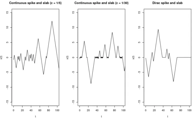
We can apply current PDMPs, such as ZigZag, to the Bayesian variable selection prob-lem if we use the continuous spike-and-slab prior (1). Realisations of such a sampler are shown in the left two plots of Figure 1 as we vary how concentrated the spike distribution is. For the more concentrated case, the sampler becomes inefficient as it involves many switching events when the state variable is close to 0.
Intuitively as we make the variance of the spike component of the prior tend to 0 the prior converges to a prior with a point mass at 0; furthermore we can observe the output of our PDMP sampler “converging” to a process shown in the right-hand plot of Figure 1. Here, rather than the state having periods where it oscillates around 0, it has periods of time where θj = 0 and thus has many fewer events.
3
Reversible Jump PDMP Samplers
Let M= (M1,M2, ...) be a set of models indexed by a parameter k. To each model Mk
correspond a state spaceXkof dimension p
k. For the sake of clarity, we will limit ourselves
to variable selection, though it is straightforward to apply the results below to more general model selection problems. In our case Xk has a specific form:
Xk =Y
i
Rγ k i
Figure 1: Sample paths of PDMPs implementing the variable selection priors in 1 dimen-sion. The left and centre plots show the trajectories for a continuous spike-and-slab prior 0.5N(0, τ2) + 0.5N(0, τ2c2) where τ2 = 16. As c decreases the spike component in the mixture approaches a Dirac mass. The figure on the right is the limiting process where we set the velocity to zero allowing the variable to stay fixed at zero.
where we abuse notation by using R0 = {0} and where (γk
i)i is a sequence of numbers
in {0,1} representing whether a variable is enabled for model Mk. Let π be the target
posterior probability defined on X =∪kXk. We further assume that the restriction of πto
each Xk has a density, and denote this by π
k(x). The first ingredient of our sampler is a
collection of PDMPs defined for each model. Each PDMP sampler adds a velocity space
Vkto the spaceXk and samples from the spaceE
k=Xk× Vk. Finally, for each modelMk,
the associated PDMP sampler has an extended infinitesimal generator Ak (Davis, 1993)
with invariant distribution proportional to νk with
νk(x,v) = πk(x)pk(v|x) (x,v)∈ Xk× Vk,
for some set of conditional densities pk(v|x).
Remark 1. For samplers such as ZigZag,pk(dv|x)is a measure with support on a discrete
set. By choosing Vk to be the support of p
integrals can be interpreted as sums over the support points. This allows us to treat all samplers within the same framework.
The second ingredient of our reversible jump PDMP sampler is a set of jumps between models. For our case of variable selection, we only allow adding or removing one variable at a time. Hence, let
T ={(i, j)| X
l
|γli−γlj|= 1 and|γi|>|γj|}
be a set of pairs of transitions between models, with these ordered (i, j) such that model
Mj being obtained from Mi by removing one of the variables in Mj. For transitioni→j,
we define an active boundary Γi,j = Xj × Vi, a subspace of Ei. Each trajectory passing
through Γi,j has some probabilitypi,j of jumping toEj using a deterministic jump function
gi,j. We assume that the jump function does not change the position. So, if a trajectory
zt of our process has a left limit at time t, zt− in Γi,j, then with some probability pi,j,
zt =gi,j(zt−)∈Ej with xt=xt−.For transition j →i, we introduce βi,j(z) a Poisson rate
and a jump kernel Qi,j(·,z) such that if the trajectory is in Ej, then with rate βi,j(zt−), zt is drawn from Qi,j(·,zt−)∈Γi,j. We impose symmetry in the jumps between models so
that for any z0 ∼Qi,j(·,z),gi,j(z0) =z.
3.1
Invariant distribution
Let ν = P
kνk be a measure on ∪kEk. The x-marginal distribution of ν is π and this
section provides conditions on Qi,j, pi,j and βi,j that has to be satisfied if ν is to be the
invariant distribution of the process. To avoid additional technicalities that complicate the proof, we gives results for PDMPs with bounded velocity spaces.
Theorem 1. Assume Vk is bounded for each k, and that we can bound the event rate over
any compact region; i.e if K ∈E is compact thenmaxz∈Kλ(z)<∞. Suppose a measure µ
is a stationary distribution with density on each Ei. Then for each function f in a suitable
set F: 0 = X i Z Ei Aifdµ+ X (i,j)∈T pi,j Z Γi,j [f(gi,j(z))−f(z)]µ(z)|hv,ni,ji|dz + X (i,j)∈T Z Ej βi,j(z) Z g−i,j1({z}) [f(z0)−f(z)]Qi,j(z0|z)dz0 ! µ(z)dz, (2)
where ni,j is the normal to Γi,j.
The setF in this theorem is the domain of the generator of our PDMP, and is described precisely in Davis (1993).
To get a directly usable conditions onβi,j, pi,j and Qi,j, some additional notation must
be introduced. When jumping from z = (x,v) ∈ Ej to z0 = (x,v0) ∈ Ei, the dimension
of the velocity vector needs to be increased by one, but the position is unchanged. Hence
g−i,j1(z) is a one-dimensional manifold, which can be related to a subset, U say, of R by introducing a function
Gi,j :U×Ej →Ei
such that for any α ∈ U, we have Gi,j(α,z) ∈ gi,j−1({z}) and for a fixed z ∈ Ej, α 7→
Gi,j(α,z) is a one to one mapping from U to g−i,j1(z) (similar ideas are seen in reversible
jump MCMC; see Green, 1995). For a givenz∈Ej, it is natural to rewrite the jump kernel
Qi,j in terms ofα ∈U, and henceforth we abuse notation and write Qi,j(·,z) as a density
on U. That is we can simulate the transition from Ej to Ei, by simulating α ∼ Qi,j(·,z)
and then setting z0 =Gi,j(α,z).
Finally, let
νi,j(z) =ν(z)|hv,ni,ji|
be an unnormalised density on Γi,j and let ¯νi,j be the pushforward measure on Ej of νi,j
by gi,j:
¯
νi,j(B) =
Z
g−i,j1(B)
νi,j(z)dz for any B ⊂Ej measurable.
Informally this is the measure under νi,j associated with values of x∈ Γi,j that would be
mapped by gi,j to the set B.
We are now in a position to give simple conditions for (2) of Theorem 1 to hold. To do this it is helpful to consider separately the cases where the space of velocities is continuous and the case where it is discrete.
Theorem 2. Assume the space of velocities is continuous. A sufficient condition for (2) of Theorem 1 to hold for ν is that, for every (i, j)∈ T, the following conditions holds
βi,j(z) =pi,j
¯
νi,j(z)
ν(z) for z∈Ej (3)
Qi,j(α|z) =
νi,j(Gi,j(α,z))|JGi,j(α,z)| ¯
νi,j(z)
for z ∈Ej and α∈U, (4)
where JGi,j denotes the Jacobian associated with the transformation Gi,j.
Intuitively, this result can be understood as a detailed balance condition: we balance the probability flow for each jump z → z0 from Ei to Ej, with that of the reverse jump
z0 →z.
For discrete velocity spaces the result is slightly simpler, as the Jacobian term is not required.
Theorem 3. Assume the velocity space is discrete. A sufficient condition for (2) of The-orem 1 to hold for ν is that, for every (i, j)∈ T, the following conditions holds
βi,j(z) = pi,j ¯ νi,j(z) ν(z) for z ∈Ej (5) Qi,j(α|z) = νi,j(Gi,j(α,z)) ¯ νi,j(z) for z ∈Ej and α ∈U. (6)
4
Example Samplers
4.1
ZigZag Sampler
We first derive the jump rates and transitions for the ZigZag sampler described in Section 2.2. For this sample the velocity of each active component is either 1 or -1, which simplifies the computation.
We choose gi,j to be the projection that sets to 0 the disabled variable. Let (i, j)∈ T
be a transition. For any v ∈ Vi, we have |hv,n
i,ji|= 1. Therefore on Ei,
νi,j(z) = ν(z) = πi(x)2−|γi|.
For z∈Ej, since a velocity component in{−1,1} is projected to 0,
¯
νi,j(z) = 2πi(x)2−|γi|=πi(x)2−|γj|.
For the jump to Ei we change the velocity for the component of the model that is added,
whilst the other components of the velocity is unchanged. Denoting the new velocity of the added component by α, we have from Theorem 3 that
βi,j =pi,j
πi(x)
πj(x)
Qi,j(α|z) = 1/2 for α∈ {−1,1}.
For our variable selection problem, the ratio of the posterior density that appears in βi,j
will simplify to the ratio of the priors as the likelihood terms are common and cancel. If we have independent priors on the parameters for each variable this term will be a constant, which simplifies the simulation of the events at which we add new variables into our model. This comment applies also to the rates for the Bouncy Particle Sampler which we derive next.
4.2
Bouncy Particle Sampler
We consider two versions of the Bouncy Particle Sampler. The first version has velocities on the unit sphere, so
Vi ={v ∈
R|γ k|
Like the ZigZag sampler, the deterministic dynamics are given by a constant velocity model. The event rate for sampling from a density πk(x) is
λ(z) = max{0,−v· ∇xlogπk(x)},
with the velocity reflecting in the normal to logπk(x) at an event. The Bouncy particle
also often has refresh events, at which a completely new velocity is sampled.
Extending the Bouncy Particle Sampler to the variable selection problem requires a more careful analysis than for the ZigZag sampler due to the geometry of the velocity space. For the jump to Ei, we will let α denote the new velocity for the component added to the
model. To ensure the new velocity lies on the unit sphere, we re-scale the other components of the velocity: so if the old velocity is v then the new velocity is αni,j +
√
1−α2v. The following proposition states how to choose the jump rate, βi,j and the density for α. Proposition 1. For the Bouncy Particle Sampler with velocities on the unit sphere, (3) and (4) are satisfied if, for all (i, j)∈ T with |γj|>0:
βi,j =pi,j πi(x) πj(x) 2Asphere(|γj|) Asphere(|γi|) 1 |γj| (7) Qi,j(α|z) = |α||γj|√1−α2|γj|−2 2 for z ∈Ej and α∈(−1,1) (8) with Asphere(|γi|) = Γ(|γi|2 ) 2π |γi| 2
the area of the unit sphere ofR|γi|; and if for |γj|= 0, where the Bouncy Particle Sampler and ZigZag are equivalent, we use the ZigZag rates.
The second version of the Bouncy Particle Sampler has velocities in R|γk|
, with their density being standard Gaussian and independent of x. The dynamics are as previously. This sampler does not satisfy our requirement that the velocity space is bounded, though the argument behind Theorem 1 can be extended to this sampler, and our results would apply to this sampler if we replaced the Gaussian density by a truncated Gaussian (with any arbitrarily large truncation value).
For the jump toEi, we again letα denote the new velocity for the component added to
the model, whilst for this version the other components of the velocity remain unchanged. Proposition 2. For the Bouncy Particle Sampler with Gaussian velocities, (3) and (4) are satisfied if, for all (i, j)∈ T:
βi,j =pi,j πi(x) πj(x) 2 √ 2π (9) Qi,j(α|z) = 2|α|e− 1 2α2 for z ∈E j and α∈R. (10)
5
Simulation Study
In this section we demonstrate the potential advantage of our new samplers compared to alternative approaches for Bayesian variable selection. To compare between different samplers we consider the Monte Carlo estimates of the posterior probabilities of inclusion, the posterior means for the regression coefficients, and the posterior means conditioned on the model. Similar comparisons methods are used in Zanella and Roberts (2019) for comparing efficiency of MCMC methods on Bayesian variable selection problems. For a given sampler the statistical efficiency is measured by the mean squared error of the sampler denoted by σ2
sampler and is calculated usingR runs of the sampler as
σsampler2 = 1 R R X i=1 (ˆqr−q)2 (11)
where ˆqr for r = 1, ..., R are the estimates of a quantity of interest from the R runs,
and q is either the exact posterior quantity of interest, if available, otherwise it is the estimate from an independent long run of an MCMC method. In multiple dimensions the statistical efficiency is measured as the median σ2
sampler over all dimensions. To compare the performance of different samplers we also consider a measure of efficiency relative to a reference sampler. If we denote the reference sampler by ref, then we define Relative Statistical Efficiency (RSE) and Relative Efficiency (RE) by
RSE = σ 2 ref nref σ2 sampler nsampler , RE = σ 2 ref tref σ2 sampler tsampler ,
where nsampler and nref are the number of iterations of the algorithms and tsampler and tref are the computation times of the algorithms. The RSE measures the relative efficiency of the algorithms per iteration whereas the RE measures the efficiency per second. For interpretation an RSE or RE value of 2 implies that the sampler is 2 times more efficient than the reference method. The sensitivity of the methods to the choice of reversible jump parameters pi,j and regular PDMP tuning parameters is explored empirically on a simple
model in the Supplementary Material. Based on these results we fixed pi,j = 0.6 for all i
and j in all reversible jump PDMP samplers and fixed the refreshment rate at 0.1 for the reversible jump BPS methods for the following results.
5.1
Logistic regression
First we compare PDMP based samplers with a collapsed Gibbs sampler and a reversible jump sampler on a logistic regression problem. The Gibbs sampler is based on the Polya-Gamma sampler of Polson et al. (2013): details of this sampler are given in the Supple-mentary Material. We implemented reversible jump MCMC using the NIMBLE software package (de Valpine et al., 2017, 2020) using independent Normal proposal for selected
variables.
The logistic regression model has a p-dimensional regression parameter θ ∈ Rp, and a
binary response yi ∈ {0,1} which is distributed as
P(yi = 1|xi,θ) =
exp(Pp
j=1xi,jθj) 1 + exp(Pp
j=1xi,jθj)
wherexi is thep-vector of covariates for observationi. In our simulation study, each vector
xi is simulated from a multivariate Normal with mean zero and p×pcovariance matrix Σ.
We use a prior that is independent for eachθj and whereθj ∼ 10pN(0,10)+(1−10p)δ0, which corresponds to a prior that favors models with 10 selected variables. Data was generated using this model and the following choices for θ and covariance matrix Σ:
1. A pair of correlated covariates, one of which is in the model: θ = (1,0, ...0)T with
Σ2,1 = Σ2,1 = 0.9, with Σi,i= 1 and Σi,j = 0 ifi6=j.
2. Structured correlation between all covariates with six active covariates:
θ = (3,3,−2,3,3,−2,0, ...,0)T with Σi,j = exp(−|i−j|).
3. No correlation between covariates and six active covariates:
θ = (3,3,−2,3,3,−2,0, ...,0)T, with Σi,i = 1 and Σi,j = 0 ifi6=j.
These simulation scenarios are analogous to others previously considered in the litera-ture for linear regression. Scenarios 1 and 3 are are similar to considered by Wang et al. (2011) and Zanella and Roberts (2019) while Scenario 2 is similar to one considered by Yang et al. (2016). We present results for both ZigZag and the Bouncy Particle Sampler with Gaussian distributed velocities (almost identical results are obtained for the Bouncy Par-ticle Sampler where the velocities are on the unit sphere). See Section D of the Appendix for more details.
The PDMP methods are competitive with Gibbs sampling in low sample sizes and offer substantial efficiency gains for larger sample sizes. Smaller gains can also be seen when the dimension is increased with fixed sample size. Both BPS and ZigZag methods offer similar relative efficiencies across the experiments. The greatest efficiency gains for reversible jump PDMP methods was seen in Scenario 1 with Scenarios 2 and 3 offering lower gains in performance. This may be due to smaller models being more likely in Scenario 1 and thus less computational effort required for the PDMP methods in gradient calculations and simulation of event times. For all experiments the Gibbs sampler offers a computational advantage over the reversible jump methods in relative efficiency for marginal posterior probabilities of inclusion. This increased performance is unsurprising as the model update steps in the Gibbs sampler have marginalised over the parameter valuesθ yielding efficient moves through the model space. In more general settings where it is not possible to integrate over θ the mixing will be substantially poorer.
The use of subsampling methods for Bayesian variable selection problems is a recently emerging area (Song et al., 2020; Buchholz et al., 2019) though it remains under-studied.
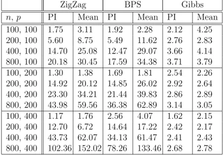
Table 1: Scenario 1 (pair of correlated variables): Relative efficiencies (RE) for meth-ods, against a Reversible Jump algorithm, for the marginal posterior means (Mean) and marginal posterior probabilities of inclusion (PI).
ZigZag BPS Gibbs
n, p PI Mean PI Mean PI Mean
100, 100 1.75 3.11 1.92 2.28 2.12 4.25 200, 100 5.60 8.75 5.49 11.62 2.76 2.83 400, 100 14.70 25.08 12.47 29.07 3.66 4.14 800, 100 20.18 30.45 17.59 34.38 3.71 3.79 100, 200 1.30 1.38 1.69 1.81 2.54 2.26 200, 200 14.92 20.12 14.85 26.02 2.92 2.64 400, 200 23.30 34.21 21.44 39.83 2.86 2.89 800, 200 43.98 59.56 36.38 62.89 3.14 3.05 100, 400 1.17 1.76 2.56 4.07 1.62 2.15 200, 400 12.70 6.72 14.64 17.22 2.42 2.17 400, 400 43.73 62.07 34.13 61.47 2.41 2.43 800, 400 102.36 152.02 78.26 133.46 2.68 2.78
Table 2: Scenario 2 (General correlation): Relative efficiency (RE) for methods, against a Reversible Jump algorithm, for the marginal posterior means (Mean) and marginal poste-rior probabilities of inclusion (PI).
ZigZag BPS Gibbs
n, p PI Mean PI Mean PI Mean
100, 100 0.57 0.83 1.15 1.86 1.05 0.76 200, 100 0.88 0.92 1.71 2.10 1.96 1.27 400, 100 1.39 1.50 2.11 2.32 1.69 1.00 800, 100 4.77 7.30 5.63 9.71 1.99 1.78 100, 200 0.76 1.21 2.03 3.03 1.53 1.37 200, 200 2.28 2.80 4.87 6.84 1.92 1.31 400, 200 4.10 4.51 6.77 8.77 1.30 0.87 800, 200 10.36 13.23 11.12 19.21 1.41 1.12 100, 400 1.09 1.27 2.93 4.01 1.12 0.88 200, 400 3.57 3.37 6.57 7.21 1.24 0.66 400, 400 8.05 8.65 13.45 16.24 1.15 0.83 800, 400 26.93 34.41 28.71 51.59 1.32 1.20
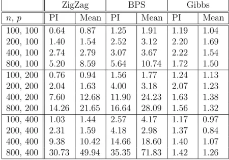
Table 3: Scenario 3 (No correlation): Relative efficiency (RE) for methods, against a Re-versible Jump algorithm, for the marginal posterior means (Mean) and marginal posterior probabilities of inclusion (PI).
ZigZag BPS Gibbs
n, p PI Mean PI Mean PI Mean
100, 100 0.64 0.87 1.25 1.91 1.19 1.04 200, 100 1.40 1.54 2.52 3.12 2.20 1.69 400, 100 2.74 2.79 3.07 3.67 2.22 1.54 800, 100 5.20 8.59 5.64 10.74 1.72 1.50 100, 200 0.76 0.94 1.56 1.77 1.24 1.13 200, 200 2.04 1.63 4.00 3.18 2.07 1.23 400, 200 7.60 12.68 11.90 24.23 1.63 1.38 800, 200 14.26 21.65 16.64 28.09 1.56 1.32 100, 400 1.03 1.44 2.57 4.17 1.17 0.97 200, 400 2.31 1.59 4.18 2.98 1.37 0.84 400, 400 9.38 10.42 14.66 18.60 1.40 1.07 800, 400 30.73 49.94 35.35 71.83 1.42 1.26
One of the attractions of PDMP samplers is that they can be implemented in a way where they only access a small subset of data at each iteration, whilst still targeting the true posterior. We now investigate how these ideas work in the variable selection problem, by comparing the efficiency of three implementations of ZigZag with that of the Gibbs sampler, and see how this depends on the number of observations. These are ZigZag using the full data, ZigZag using subsampling with a global bound, and ZigZag with subsampling control variates (see Bierkens et al., 2019, for details of both subsampling approaches).
Standard application of control variates requires calculation of the gradient at a ref-erence point using the full likelihood. Due to the trans-dimensional nature of variable selection problems, a full gradient calculation is not well defined. For this reason we choose to make use of control variates defined for a fixed model M where the gradient is well defined. These control variates are only used when the sampler is in this model. Exten-sions where multiple control variates are used for models with high probability would be straightforward.
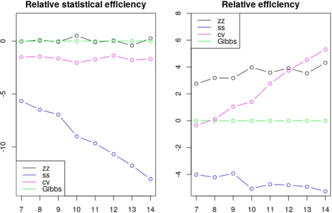
Results are shown in Figure 2. Despite our simplistic implementation, these results indicate that Zig-Zag with control variates is becoming increasingly efficient relative to Zig-Zag using the full dataset as the number of samples increases. Furthermore we see evidence of super-efficiency – whilst the computational cost per ESS of the Gibbs sampler is expected to be linear in the number of observations, the relative efficiency plots suggest that this is sub-linear for ZigZag with control variates.
Figure 2: Log-log plots of efficiency, relative to the Gibbs sampler, of different samplers as we vary the number of observations. Plotted are the relative efficiencies for the posterior mean conditional on model M∗ where M∗ corresponds to the true data generated model.
The dataset was generated with a 15-dimensional regression parameterθ = (1,1,0,0, ...,0). The methods run are the Zig-Zag applied to the full dataset (zz, black), Zig-Zag with subsampling using global bounds (ss, blue), Zig-Zag with control variates (cv, magenta) and Gibbs sampling (Gibbs, green). All methods were initialised at the location of the control variate. Methods were given the same computational budget, for details see Section D of the Appendix.
5.2
Robust regression
As mentioned in the introduction, a common approach to Bayesian variable selection is to use continuous spike-and-slab priors for each parameter rather than try to sample from the joint posterior of model and parameters. Such an approach is attractive as it enables standard gradient-based samplers, such as Hamiltonian Monte Carlo, to be used. We now compare such an approach, implemented with the popular STAN software (Carpenteret al., 2017), to our PDMP samplers. Our aim is to both investigate the computational efficiencies of the two approaches and to show the differences in posterior that we obtain from these different types of prior. Our comparison is based on a robust linear regression model.
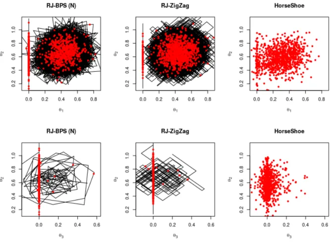
Figure 3: Dynamics of the samplers on a robust regression example with spike and slab or horseshoe prior. The top row shows the posterior for θ1 and θ2, bottom row shows the estimates for θ2 and θ3. The spike and slab distributions are sampled using the reversible jump PDMP samplers with reversible jump parameter 0.6 and refreshment for the BPS methods set to 0.5. All methods are shown with 103 samples (red) and the PDMP dynamics are shown in black. Sampling with the Horseshoe prior was implemented in Stan using NUTS. Both Stan and PDMP methods were run for the same computing time. To aid visualisation only the first 30% of the PDMP trajectories are shown.
In particular, we model the errors in our linear regression model as a mixture of Normals with different variances. Thus
Y = p X i=1 Xjθj+, ∼ 1 2N(0,1) + 1 2N(0,10 2 ).
and Vehtari, 2017a,b) θj ∼N(0, τ2λ˜j), λ˜j = c2λ j c2+τ2λ j , λj ∼C+(0,1)
for j = 1, ..., p where C+(0,1) denotes the half-Cauchy distribution for the standard devi-ation λj. The regularised horseshoe is a variation of the horseshoe prior (Carvalho et al.,
2010) that offers a continuous approximation of a Dirac spike and slab where the slab is a Normal distribution with finite variance c2. The hyper-parameter τ controls the global shrinkage of the variables towards zero. In Carvalho et al. (2010) it was shown that for standard linear regression the optimal choice for a fixed value of τ is τ0 =σ(p−pp00)√n where
p0 is a the number of nonzero variables in the sparse model and σ is the noise variance. In line with this, we compare the regularised horseshoe prior with fixed hyper-parameter
τ0 = (p−pp0
0) √
n against the spike-and-slab prior
θj ∼ p0 pN(0, c 2) + 1−p0 p δ0
for j = 1, ..., p. MCMC for the model using a horseshoe prior was performed by Stan’s implementation of NUTS (Hoffman and Gelman, 2014).
We first compare the variable selection dynamics for a simple model withp= 4 variables,
n = 120 observations and regression parameter θ = (0.5,0.5,0,0)T. The covariate values
and residuals were generated as independent draws from a standard Normal and the prior expected model size is set to p0 = 1. Example output for the PDMP samplers and the Stan implementation is shown in Figure 3. The posteriors show the horseshoe prior replicating the effect of the spike-and-slab through shrinking the coefficients towards zero, but it is not able to give exact zeros.
We now compare the reversible jump PDMP methods in terms of their sampling effi-ciency for a higher dimensional problem. The dataset is generated forp= 200 variables and
n = 100 observations with regression parameter θ = (2,2,2,2,0,0,0....0)T. The covariates
for each observation were drawn from an AR(1) process with lag-1 correlation of 0.5. The residuals were generated from a standard Cauchy distribution.
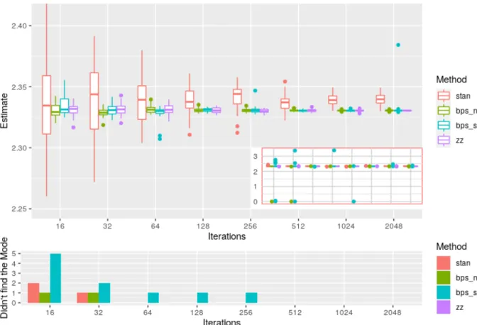
We ran Stan with the default settings for a burnin of 1000 iterations and then for 16, 32, 64, ..., 2048 iterations. We ran the reversible jump PDMP samplers for the same wall clock time for both burnin and subsequent iterations. The experiment was repeated 35 times and the resulting boxplots of the posterior mean of θ1 are shown in Figure 4.
Figure 4: Sampling efficiency for reversible jump PDMP vs Stan for the robust regression example. The top figure is boxplots of the posterior mean ofθ1for increasing computational budget, with outliers from the sampler removed for visualisation purposes. These removed outliers correspond to times that the sampler has become stuck in a local mode where
θ1 = 0. The subplot shows the full results including outliers from the sampler. Both the Stan and reversible jump PDMP methods converge to similar solutions despite having different priors. The bottom figure shows the number of times that the samplers did not find the global mode.
For the same computational budget, the reversible jump PDMP methods are able to attain better performance. However, it is also apparent from this simulation that the BPS reversible jump PDMP methods are more sensitive to local modes. It is unclear if this is an artifact of the sampler or due to the choice of refreshment rate (0.6). This sensitivity is seen to diminish as the sampler is run for longer.
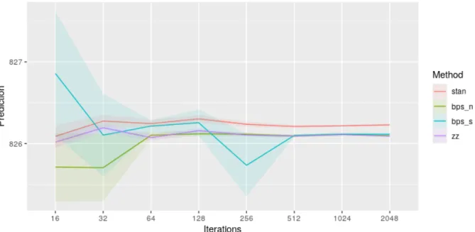
The predictive ability of the methods is compared in Figure 5. Here an additionaln= 100 observations were drawn from the same model and these were used as a hold-out dataset to validate the posterior predictive ability. The predictive ability is defined in terms of the Monte Carlo estimate of the mean square prediction performance 1001 P100
i=1(yi−xTiθ)2where
of time for the reversible jump PDMP samplers. The reversible jump PDMP samplers all give the same predictive performance for large iteration numbers while Stan, which uses a horseshoe prior, performs slightly worse.
Figure 5: Predictive ability of reversible jump PDMP vs Stan for the robust regression example. The predictive ability is measured by Monte Carlo estimates of the mean square predictive performance.
6
Discussion
We have shown how PDMP samplers can be extended so that they can sample from the joint posterior over model and parameters in variable selection problems. There are a number of open challenges that stem from this work. First, as with any MCMC algorithm, the reversible jump PDMP samplers have tuning parameters. Our simulation results were based on choosing these after empirically evaluating the performance of the samplers on one simple problem. Whilst the samplers mixed well, it is likely that better mixing could be achieved if more informed choices of tuning parameters were made, and theory for guiding such choices is needed.
Second, the form of our reversible jump PDMP samplers is based on particularly features of the variable selection problem. In other model choice settings, different trans-dimensional moves may be needed. The theory we developed should be able to be adapted to give rules for choosing rates of such moves. Also our trans-dimensional moves are reversible, that is they balance probability flow from modelito modelj by the flow of probability from model
be constructed.
Third, it is likely that the reversible jump PDMP samplers will still struggle in situations where the posterior is multi-modal with well separated modes. For such cases it would be interesting to try and incorporate ideas such as tempering (Marinari and Parisi, 1992) to allow for better mixing across modes. Also given the close links between PDMP samplers and Hamiltonian Monte Carlo, it would be interesting to see if the ideas we have presented for trans-dimensional jumps could be adapted to be used with Hamiltonian Monte Carlo algorithms.
References
Bierkens, J. and Roberts, G. (2017). A piecewise deterministic scaling limit of lifted Metropolis–Hastings in the Curie–Weiss model.The Annals of Applied Probability 27(2), 846–882.
Bierkens, J., Bouchard-Cˆot´e, A., Doucet, A., Duncan, A. B., Fearnhead, P., Lienart, T., Roberts, G. and Vollmer, S. J. (2018). Piecewise deterministic Markov processes for scalable Monte Carlo on restricted domains. Statistics & Probability Letters 136, 148– 154.
Bierkens, J., Fearnhead, P., Roberts, G.et al.(2019). The zig-zag process and super-efficient sampling for Bayesian analysis of big data. The Annals of Statistics 47(3), 1288–1320. Bierkens, J., Grazzi, S., Kamatani, K. and Roberts, G. (2020). The boomerang sampler.
arXiv:2006.13777 .
Bottolo, L. and Richardson, S. (2010). Evolutionary stochastic search for bayesian model exploration. Bayesian Analysis 5, 583–618.
Bouchard-Cˆot´e, A., Vollmer, S. J. and Doucet, A. (2018). The bouncy particle sampler: A nonreversible rejection-free Markov chain Monte Carlo method.Journal of the American Statistical Association 113(522), 855–867.
Buchholz, A., Ahfock, D. and Richardson, S. (2019). Distributed computation for marginal likelihood based model choice. arxiv.1910.04672 .
Carpenter, B., Gelman, A., Hoffman, M. D., Lee, D., Goodrich, B., Betancourt, M., Brubaker, M., Guo, J., Li, P. and Riddell, A. (2017). Stan: A probabilistic program-ming language. Journal of Statistical Software 76(1).
Carvalho, C. M., Polson, N. G. and Scott, J. G. (2010). The horseshoe estimator for sparse signals.Biometrika 97(2), 465–480.
Chipman, H. A., George, E. I. and McCulloch, R. E. (2001). The practical implementation of Bayesian model selection (with discussion). Model Selection (P. Lahiri ed.) , 65–134. Davis, M. (1993). Markov Models and Optimization. Chapman Hall.
de Valpine, P., Turek, D., Paciorek, C., Anderson-Bergman, C., Temple Lang, D. and Bodik, R. (2017). Programming with models: writing statistical algorithms for general model structures with NIMBLE.Journal of Computational and Graphical Statistics 26, 403–413.
de Valpine, P., Paciorek, C., Turek, D., Michaud, N., Anderson-Bergman, C., Obermeyer, F., Wehrhahn Cortes, C., Rodr`ıguez, A., Temple Lang, D. and Paganin, S. (2020). NIMBLE User Manual. R package manual version 0.10.0.
Diaconis, P., Holmes, S. and Neal, R. M. (2000). Analysis of a nonreversible Markov chain sampler. Annals of Applied Probability 10, 726–752.
Fearnhead, P., Bierkens, J., Pollock, M. and Roberts, G. O. (2018). Piecewise deterministic Markov processes for continuous-time Monte Carlo. Statistical Science 33(3), 386–412. George, E. I. and McCulloch, R. E. (1993). Variable selection via gibbs sampling. Journal
of the American Statistical Association 88(423), 881–889.
Geweke, J. (1996). Variable selection and model comparison in regression. In: Bayesian Statistics 5, Oxford University Press, 609–620.
Green, P. J. (1995). Reversible jump Markov chain Monte Carlo computation and Bayesian model determination. Biometrika 82(4), 711–732.
Hoffman, M. D. and Gelman, A. (2014). The No-U-Turn sampler: adaptively setting path lengths in Hamiltonian Monte Carlo.Journal of Machine Learning Research 15(1), 1593– 1623.
Ishwaran, H. and Rao, J. S. (2005). Spike and slab variable selection: frequentist and Bayesian strategies.The Annals of Statistics 33(2), 730–773.
Kuo, L. and Mallick, B. K. (1998). Variable selection for regression models.Sankhya Series B 60, 65–81.
Marinari, E. and Parisi, G. (1992). Simulated tempering: a new Monte Carlo scheme.EPL (Europhysics Letters) 19(6), 451.
Markovic, J. and Sepehri, A. (2018). Bouncy hybrid sampler as a unifying device. arXiv:1802.04366 .
Michel, M., Kapfer, S. C. and Krauth, W. (2014). Generalized event-chain Monte Carlo: Constructing rejection-free global-balance algorithms from infinitesimal steps.The Jour-nal of Chemical Physics 140(5), 054116.
Michel, M., Durmus, A. and S´en´ecal, S. (2020). Forward event-chain Monte Carlo: Fast sampling by randomness control in irreversible Markov chains.Journal of Computational and Graphical Statistics , To appear.
Mitchell, T. J. and Beauchamp, J. J. (1988). Bayesian variable selection in linear regression. Journal of the American Statistical Association 83(404), 1023–1032.
Neal, R. M. (2011). MCMC using Hamiltonian dynamics. In: Handbook of Markov chain Monte Carlo (eds. A. Brooks, A. Gelman, G. L. Jones and X. Meng), Chapman & Hall, 113–162.
Peters, E. A. and de With, G. (2012). Rejection-free Monte Carlo sampling for general potentials. Physical Review E 85(2), 026703.
Piironen, J. and Vehtari, A. (2017a). On the Hyperprior Choice for the Global Shrink-age Parameter in the Horseshoe Prior. volume 54 of Proceedings of Machine Learning Research, PMLR, 905–913.
Piironen, J. and Vehtari, A. (2017b). Sparsity information and regularization in the horse-shoe and other shrinkage priors. Electron. J. Statist.11(2), 5018–5051.
Polson, N. G., Scott, J. G. and Windle, J. (2013). Bayesian inference for logistic models using P´olya–Gamma latent variables. Journal of the American statistical Association 108(504), 1339–1349.
Smith, M. and Kohn, R. (1996). Nonparametric regression using bayesian variable selection. Journal of Econometrics 75(2), 317 – 343.
Song, Q., Sun, Y., Ye, M. and Liang, F. (2020). Extended stochastic gradient Markov chain Monte Carlo for large-scale Bayesian variable selection. Biometrika Asaa029.
Vanetti, P., Bouchard-Cˆot´e, A., Deligiannidis, G. and Doucet, A. (2017). Piecewise-Deterministic Markov Chain Monte Carlo. arXiv:1707.05296 .
Wang, S., Nan, B., Rosset, S. and Zhu, J. (2011). Random lasso. Ann. Appl. Stat. 5(1), 468–485.
Wu, C. and Robert, C. P. (2020). Coordinate sampler: a non-reversible Gibbs-like MCMC sampler. Statistics and Computing 30(3), 721–730.
Yang, Y., Wainwright, M. J. and Jordan, M. I. (2016). On the computational complexity of high-dimensional bayesian variable selection.Ann. Statist. 44(6), 2497–2532.
Zanella, G. and Roberts, G. (2019). Scalable importance tempering and bayesian variable selection. Journal of the Royal Statistical Society: Series B (Statistical Methodology) 81(3), 489–517.
Supplementary Material: Reversible Jump PDMP
Samplers for Variable Selection
A
Proofs
A.1
Proof of Theorem 1
Recall theorems 34.15 and 34.19 from Davis (1993):
Theorem 4 (34.15). Suppose that µis a stationary distribution for (xt). Then there exists
a finite measure σ on Γ (the active boundary) such that for all t >0: Eµ 1 t Z t 0 f(xs−)dp∗ s = Z Γ f(x)σ(dx)
where p∗ is the counting process that counts the number of jumps for the boundary
Theorem 5 (34.19). Suppose µ is a stationary distribution for (xt) and let σ be the
cor-responding boundary measure defined above. Then:
Z E Af(x)µ(dx) + Z Γ Cf(z)σ(dz) = 0 where A is the extended generator and Cf = (Qf −f).
Remark 2. The construction of PDMPs with an active boundary we presented differs slightly from the one found in (Davis, 1993, p. 57). However our process still fits the definition of Davis (1993): one simply needs to separate each Xk in two at the boundary
and consider the two parts as two separated spaces.
From the expression of the extended generator given in (26.14) of Davis (1993), it follows that X i Z Ei Aifdµ+ X (i,j)∈T Z Ej βi,j(z) Z g−i,j1({z}) [f(z0)−f(z)]Qi,j(z0|z) dz0 ! µ(z)dz
corresponds to the first term of Theorem 5. It is now left to show that
X (i,j)∈T pi,j Z Γi,j [f(gi,j(z))−f(z)]µ(z)|hv,ni,ji|dz
corresponds to the boundary term of Theorem 5. Following Davis (1993) notations, for a fixed (i, j) in T, the operator C= (Qf −f) where Q is the jump kernel at the boundary has the following expression:
Finally, we need to find an expression for measure σ. We start from the definition in Theorem 4: Eµ 1 t Z t 0 f(zs−)dp∗ s = Z Γi,j f(z)σ(dz),
where p∗s is the counting process that counts the number of times we hit Γi,j. This holds
for all t, and we will derive σ by considering the value of the left-hand side as t → 0. Intuitively the idea is that, in this limit, the impact of the events will be negligible and we can evaluate the left-hand side by considering a process where z0 is simulated from µ but then is purely deterministic, with dynamics given by the deterministic part of the PDMP. As indicator functions of compact sets separate measures on Γi,jwe can restrict ourselves
to these functions. Let K be a compact of Γi,j and f its characteristic function, f = 1K.
We also introduce some additional notation. Let ˜zt be a deterministic process that follows
the dynamics of the deterministic part of the PDMP, and let ˜p∗t be the associated process that counts the number of times ˜zt hits Γi,j. For our PDMP let Ω0(t) be the set of paths for which no events occur by time t, and Ω1(t) the set of paths with at least one event prior to time t. We can write
Z t 0 1K(zs−)dp∗s = Z t 0 1K(zs−)1Ω 0(t)dp ∗ s + Z t 0 1K(zs−)1Ω 1(t)dp ∗ s,
that is split the integral into two, with the first being the contribution from paths with no event and the second the contribution of paths with at least one event.
We now introduce two sets. Let Kt ={z ∈E|zs ∈ K with z0 =z and s ∈[0, t]}, and ˜
Kt ={z ∈Ei|z˜s ∈K with ˜z0 =z and s∈[0, t]}. The first is the set of all possible starting points for our PDMP process for which it is possible to hit K by time t, the latter is the same set but for the purely deterministic process (equivalently, all PDMP paths with no events by timet). As K is compact so is ˜Kt. Furthermore as the velocity space is bounded
and K is compact so is Kt. This, together with our assumption on the event rate means
that we can upper bound the event rate for both z ∈ Kt and z ∈K˜t, and denote such an
upper bound by λ+. Now Eµ
Rt
01K(zs−)1Ω1(t)dp ∗
s can be bounded as for the integral to be non-zero we need
z0 ∈Ktand the number of times the PDMP hits Γi,j is at most twice the number of events.
Thus an upper bound is 2λ+tPr
µ(z0 ∈Kt). As the volume of Kt tends to 0 as t→0, this
upper bound is o(t).
To bound the contribution from the other integral, we notice that we can bound this from above by the the PDMP process without events, and from below by using our bound on the event rate. Thus
Eµ Z t 0 1K( ˜zs−)d˜p∗s ≥Eµ Z t 0 1K(zs−)1Ω 1(t)dp ∗ s ≥exp{−tλ +} Eµ Z t 0 1K( ˜zs−)d˜p∗s. Thus Eµ Z t 0 1K(zs−)1Ω 1(t)dp ∗ s =Eµ Z t 0 1K( ˜zs−)d˜p∗s+o(t).
Thus, for any compact subset of Γi,j, K, we have Z Γi,j 1K(z)σ(dz) = lim t→0Eµ 1 t Z t 0 1K(zs−)dp∗s = lim t→0Eµ Z t 0 1K( ˜zs−)d˜p∗s.
The final step is to obtain limt→0Eµ
Rt
0 1K( ˜zs−)d˜p
∗
s, which comes from the following
result for solutions of ordinary differential equations:
Theorem 6. Let E be a subset of Rd, µ a measure with a density with respect to the Lebesgue measure of E and letX be the vector field associated to the order ordinary differ-ential equation
d(zt)
dt =X(zt).
Let H be an hyperplane of E with normal nH and t∗(z) be the first hitting time of a
trajectory with H starting from z. Assuming there exists a measure σ on H such that for all f :H →R: lim t→0 1 t Z E f(zt∗(z0))1t∗(z0)≤tµ(z0)dz0 = Z H f(z)σ(z)dz
then σ has a density with respect to the Lebesgue measure of H and
σ(dz) =µ(z)|hz,nHi|dz
For completeness, this result is proven in Appendix A.6. The intuition behind the
|hz,nHi|factor is that ‘area’ of space that hitsz within an infinitesimal time interval dtis
|hz,nHi|dt.
Applying this theorem to the deterministic part of our PDMP we get
σ(z)dz =µ(z)|hv,ni,ji|dz
where ni,j is the normal the the boundary Γi,j, which concludes the proof.
A.2
Proof of Theorem 2
Proof. The core of the proof is rewriting (2) of Theorem 1 in a more suitable way. First, notice that Z Γi,j f(gi,j(z))µ(z)|hv,ni,ji|dz = Z Ej f(z)¯νi,j(z) dz
by definition of the pushforward measure ¯νi,j. Second, since Qi,j integrates to 1, we get:
Z Ej βi,j(z) Z g−i,j1({z}) f(z)Qi,j(z0|z) dz0µ(z) dz = Z Ej βi,j(z)f(z)µ(z) dz.
Third, using the definitions of Gi,j Z gi,j−1({z}) f(z0)Qi,j(z0|z) dz0 = Z U f(Gi,j(α,z))Qi,j(α|z) dα
Finally, using a change the change of variable from z0 = (x0,v0) to α,z defined as z0 =
Gi,j(α,z), and the definition of νi,j:
Z Γi,j f(z0)ν(z0)|hv0,ni,ji|dz0 = Z Ej Z U
f(Gi,j(α,z))νi,j(G(α,z))|JGi,j(α,z)|dαdz. Thus (2) of Theorem 1, evaluated for π =ν, can be restated as:
0 =X i Z Ei Aifdν+ X (i,j)∈T Z Ej
[pi,jν¯i,j(z)−βi,j(z)ν(z)]f(z)dz
+ X (i,j)∈T Z Ej Z U
βi,j(z)Qi,j(α|z)ν(z)−pi,jνi,j(Gi,j(α,z))|JGi,j(α,z)|
f(Gi,j(α,z)) dαdz
(12) By construction, for any function f ∈ F:
X
i
Z
Ei
Aifdν = 0.
Conditions 3 and 4 of the theorem clearly imply that
X
(i,j)∈T Z
Ej
[pi,jν¯i,j(z)−βi,j(z)ν(z)]f(z)dz= 0
and X (i,j)∈T Z Ej Z U
βi,j(z)Qi,j(α|z)ν(z)−pi,jνi,j(Gi,j(α,z))|JGi,j(α,z)|
f(Gi,j(α,z)) dαdz= 0
respectively, which concludes the proof.
A.3
Proof of Theorem 3
Proof. The proof is largely the same as the proof of Theorem 2. The only change is how to treat the change of variable z0 = Gi,j(α,z). First, notice that Gi,j leaves the position
invariant since gi,j leaves the position invariant. Then, since the velocity space is discrete
and α 7→Gi,j(α,z) is a one to one mapping for a fixedz ∈Ej:
Z Γi,j f(z0)νi,j(z0)|hv0,ni,ji|dz0 = Z Xj X v0∈Vi f(x0,v0)νi,j(x0,v0) dx0 = Z Xj X v∈Ej X α∈U
which we can write in integral form as Z Γi,j f(z0)νi,j(z0)|hv0,ni,ji|dz0 = Z Ej Z U
f(Gi,j(α,(x,v))νi,j(Gi,j(α,(x,v))) dαdz.
A.4
Proof of Proposition 1
Proof. Here: Vi ={v ∈ R|γ i| such thatkvk= 1} For z∈Ei: ν(z) =πi(x) 1 Asphere(|γi|) with Asphere(|γi|) = Γ(|γi|2 ) 2π |γi| 2
the area of the unit sphere of R|γi|.
In this case we can define Gi,j : (−1,1)×Ej → Ei such that z0 = (x0,v0) =Gi,j(α,z),
where z = (x,v), as x0 =x and v0 =√1−α2v+αn i,j. LetB ⊂ Vj Z B ¯ νi,j(x,v)dv=πi(x) Z g−i,j1(B) |<v0,ni,j >| 1 Asphere(|γi|) dv0 =πi(x) 1 Asphere(|γi|) Z [−1,1]×B |<√1−α2v+αn
i,j,ni,j >||JGi,j|dαdv = 2πi(x) 1 Asphere(|γi|) Z (0,1]×B α|JGi,j|dαdv,
where the last inequality uses the symmetry of the integral with respect to α, and that
<v,ni,j >= 0 by definition of velocities in Ej.
The determinant of Gi,j must be carefully computed since the velocities lives in the
sphere and not on the full vector space. We get:
|JGi,j(α,v)|= √ 1−α2|γ j|−2 . Therefore for |γj|>0: ¯ νi,j(z) = πi(x) 2 Asphere(|γi|) . 1 |γj|
Hence for |γj|>0: βi,j =pi,j πi(x) πj(x) 2Asphere(|γj|) Asphere(|γi|) 1 |γj|, (13) and Qi,j(α|z) = |α||γj|√1−α2|γj|−2 2 forz ∈Ej and α∈(−1,1) (14) For |γj|= 0, BPS and ZigZag are equivalent, thus we use ZigZag rates.
A.5
Proof of Proposition 2
Proof. Here: Vi =R|γi| Therefore, for z ∈Ei: ν(z) = πi(x) 1 (2π)|γi|2 e−12kvk 2
For (i, j)∈ T with|γj|>0, we can defineG
i,j : (−1,1)×Ej →Ei such thatz0 = (x0,v0) =
Gi,j(α,z), where z= (x,v), as x0 =x and
v0 =v+αni,j.
Clearly, we have |JGi,j(α,z)|= 1. Let B ⊂ V
j Z B ¯ νi,j(x,v)dv =πi(x) Z g−i,j1(B) |<v0,ni,j >| 1 (2π)|γi|2 e−12kvk2dv0 =πi(x) 1 (2π)|γi|2 Z R×B |<v+αni,j,ni,j >|e− 1 2kv+αni,jk 2 |JGi,j|dαdv =πi(x) 1 (2π)|γi|2 Z R×B |α|e−12(α 2+kvk2) dαdv =πi(x)2 1 (2π)|γi|2 Z B e−12(kvk 2) dv. Therefore for |γj|>0: ¯ νi,j(z) = πi(x)2 1 (2π)|γi|2 e−12(kvk 2) ,
and βi,j =pi,j πi(x) πj(x) 2 √ 2π (15)
Furthermore, |JGi,j|= 1 thus:
Qi,j(α|z) = 2|α|e−
1 2α
2
for z ∈Ej and α ∈R (16)
A.6
Proof of Theorem 6
Proof. LetZ(t,z) be the flow associated to the ODE. Fixz0inHsuch thata=hX(z0),nHi 6=
0. In order to show that σ has the required form it is enough to prove that lim
r→0
σ(H∩B(z0, r)) VolumeH(H∩B(z0, r))
=|a|µ(z0)
where B(z0, r) is the ball of radius r centered on z0, H ∩B(z0, r) is the slice of this ball that lies on H, and VolumeH is the Lebesgue measure of the hyperplane H.
Forr and t >0, let
Er,t ={z ∈E : 0≤t∗(z)≤t, Z(t∗(z),z)∈B(z0, r)∩H}
We can re-write the definition of σ in terms of Er,t, from which we are reduced to show
that lim r→0limt→0 1 tµ(Er,t) VolumeH(H∩B(z0, r)) =|a|µ(z0)
The idea of the proof is that to calculate µ(Er,t) we need to find the volume of Er,t as
r, t→0, and we will do this by boundingEr,t from both above and below by cylinders. We
can approximated these cylinders by the set Er,t that we would obtain if X(z) = X(z0) (i.e. the derivative was constant). The following lemma enables us to quantify the order of error for such an approximation.
Lemma 1. 1. Let r0 > 0. When t > 0 is small enough, Z(s,z) ∈ B(z0, r0) for all
z ∈B(z0, r0/2) and s∈[−t, t].
2. Let e(s,z) be the function defined by e(s,z) =Z(s,z)−(z+sX(z0)). Then: lim
(s,z)→(0,z0),s6=0
1
Proof. For part (1): Z is continuous as a function fromR×E toE. Therefore for t small enough, Z(s, z)∈B(z0, r0) for all z∈B(z0, r0/2) and s∈[−t, t].
For part (2): We define
Cz0,r = sup
z∈B(z0,r)
kX(Z(s,z))−X(z0)k.
We clearly have Cz0,r <∞ and Cz0,r −−→
r→0 0. We set r0 = 2kz−z0k, and using the mean value theorem with the function ez(s) = e(s,z) whose derivative is X(Z(s,z))−X(z0) with the fact that e(0,z) = 0 implies
ke(s,z)k ≤sCz0,2kz−z0k
which concludes the proof.
The following two lemmas then give, respectively, the cylinders that lower and upper bound Er,t.
Lemma 2. For z ∈B(z0, r)∩H ands∈[−t,0], there exists a constantC > 0and function
o(r)≥0 with limr→0o(r)/r= 0 such that
Er,t ⊂(B(z0, r+tC)∩H) + [−at−o(r)t,0]nH
The addition on right-hand side of this statement should be interpreted as addition of sets on a product space. That is the set on the right-hand side is the cylinder of points that can be written as z+snH where z∈B(z0, r+tC)∩H and s∈[−at−o(r)t,0]. Proof. We have that
Er,t={Z(s,z) :−t≤s ≤0, z ∈H∩B(z0, r)}. Let z be in B(z0, r)∩H and s∈[−t,0]
Z(s,z) = z+sX(z0) +e(s,z)
=z+s(X(z0)−anH) +sanH +e(s,z)
Notice that X(z0)−anH is inH hencez+s(X(z0)−anH) is also inH. Lemma 1 allows
us to bound 1se(s,z) on [0, t]×B(z0, r)∩H which concludes the proof.
Lemma 3. For z∈B(z0, r)∩Hands∈[−t,0], there exists a constantC > 0and function
o(r)≥0 with limr→0o(r)/r= 0 such that
Proof. Let z∈B(z0, r−tC)∩H−[0, at−o(r)t]nH.
hZ(s,z),nHi=hz,nHi+sa+he(s,z),nHi
Using Lemma 1, there exists s ∈ [0, at−o(r)] (intuitively s ≈ hz0 −z,nHi/a ≤ ata = t)
such that hZ(s,z),nHi=hz0,nHi, which impliesZ(s,z)∈H. Hence z ∈Er,t.
Using Lemmas 2 and 3, we have constants C1 and C2 and a function o1(r) and o2(r) with ok(r)/r →0 (k = 1,2) such that
Volume(Er,t)
t ≥(a−o1(r))VolumeH(B(z0, r−tC1)∩H)
Volume(Er,t)
t ≤(a+o2(r))VolumeH(B(z0, r+tC2)∩H)
where Volume and VolumeH are with respect to the Lebesgue measure ofE and H
respec-tively. Since µ has continuous densities, for any > 0 there exists r0 such that for every
r < r0, µ(Er,t) t − µ(z0)Volume(Er,t) t < .
Hence for every > 0 there exists r0 > 0 and T > 0 such that for every r < r0 and 0< t < T, 1 tµ(Er,t) VolumeH(H∩B(z0, r)) − |a|µ(z0) <
which concludes the proof.
B
Sensitivity to tuning parameters
The tuning parameters for the reversible jump PDMP methods consist of: 1. the reversible jump parameter pi,j introduced in Section 3;
2. the refreshment distribution for velocities of BPS; and 3. the refreshment rateλref for BPS.
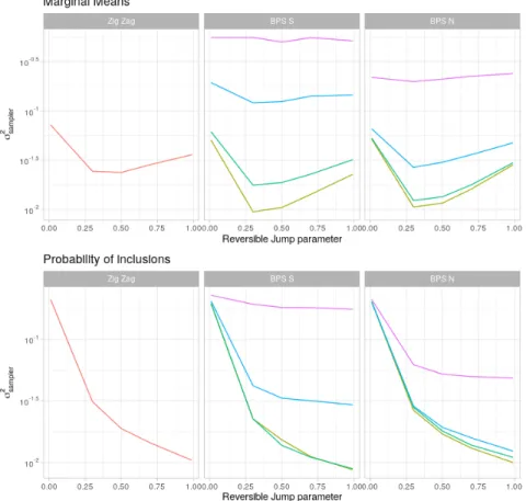
To investigate the performance of our methods we consider sampling from a 100-dimensional spike and slab distribution withθj ∼ 0.5N(0.5,1) + 0.5δ0,independently forj = 1, ...,100. Each sampler was run 100 times for a computational budget of 10.
Figure 6: Plots of the Monte Carlo variance for different samplers with varying choices of tuning parameters. The Monte Carlo variance is defined relative to the estimates of the posterior means and probabilities of inclusion.
We compare the methods based on the statistical efficiency of the estimates of marginal means and probability of inclusions. The PDMP methods appear to perform optimally in estimation of the marginal mean when they are able to spend a reasonable amount of time exploring the model space and exploring the parameter space. This can be seen in Figure 6 where optimal statistical efficiency for the marginal means occurs when pi,j is the
range 0.2 to 0.7 across all samplers. Figure 6 also shows that higher values of the reversible jump parameter pi,j gives better estimation of the probabilities of inclusions. Having a
high refreshment rate appears to impact BPS with Normal velocity distribution less than BPS with velocities distributed uniformly on the hyper-sphere. This is seen as the magenta curve (refreshment = 10) is lower for BPS N than BPS S in Figure 6 across all reversible jump parameters. All BPS methods appear to out-perform Zig-Zag in terms of marginal mean estimation when the refreshment rate is low.
C
General implementation details
Inference in Bayesian model selection relies on expectations with respect to a posterior target distribution, π(θ,γ). The parameters are θ while γ is a vector which indexes the model with elements γj = 1 if the jth variable is included and γj = 0 otherwise. The
posterior has the form
π(θ,γ)∝L(y1:n|θ,γ)π0(θ|γ)π0(γ)
where L(y1:n|θ,γ) defines a likelihood function for observations y1:n, π
0(θ|γ) and π0(γ) denote prior distribution for θ and γ. We abuse notation writing θγ to denote the
sub-vector of θ with only the elements where γj = 1. Moreover, we write π(θγ) for π(θ | γ)
where π(θ |γ) = 0 whenever |θj|>0 with corresponding γj = 0.
When simulating from the reversible jump PDMP sampler there are two types of events: normal events for the PDMP sampler within a model γ and model jump events. The standard PDMP events are taken with respect to π(θ|γ) so rates to sample are given using the usual Bouncy Particle Sampler or Zig-Zag rates on the conditioned model
λBP S(s) = −vγ · ∇θγ logπ(θγ +svγ) + , λZZi (s) = (−vi∇θilogπ(θγ +svγ)) + , for i∈ {i:γi = 1}.
In practice to simulate these events we first bound the rates by a simple function, which for the examples we consider will be linear in time. We then simulate events from a Poisson process with this linear-in-time rate, which can be done exactly, and use thinning to generate the actual events in the PDMP. Derivations of the linear-in-time bounds on the rates that we use are now given, before we give the rates for jumps between models.
C.1
Rates for logistic and robust regression
Here we give details on simulating rates for the logistic regression example. Taking a simple independent Gaussian prior the reintroduction rate simplifies to
βγ→γ0 =pγ→γ0 1 √ 2πσ2 w (1−w)
where γ and γ0 are defined as above. The standard PDMP rates are used for π(θ|γ) =
π(θγ). So to simplify notation we will assume a fixed dimension and writeθ dropping the
indexing with γ. The log posterior for both logistic and robust regression can be written in the form −logπ(θ) = n X i=1 g(ei) + θTθ 2σ2. For logistic regression ei =−xTi θ and g(ei) = −log
exp(yi) 1+exp(ei)
, and for robust regression
ei =yi−xTi θ and g(ei) =−log exp(−12e2i) +
1 10exp(− 1 200e 2 i)
event rates for the Bouncy Particle Sampler and ZigZag below.
Bouncy Particle Sampler: Let f(θ+tv) = −∇θlogπ(θ+tv) the event rate depends
on the quantity hv, f(θ+tv)i=hv, n X i=1 xTi g0(ei(t)) + 1 σ2(θ+tv)i.
where g0(ei(t)) is the derivative ofg evaluated evaluated atei(t) = −xTi (θ+tv) for logistic
regression and ei(t) =yi−xTi (θ+tv) for robust regression. The in-time derivative of this
quantity is d dthv, f(θ+tv)i=hv, n X i=1 xTi g00(ei(t))xTi v+ 1 σ2vi= n X i=1 g00(ei(t))(xTi v) 2+ 1 σ2v Tv.
If the in-time derivative can be bounded by a constant we can simulate using linear rates. For logistic regressiong00(ei)≤ 41 and for robust regression g00(ei)<1. The Bouncy Particle
Sampler rate is bounded by the linear rate
max(0,hv, f(θ+tv)i)≤max (0,hv, f(θ)i) +t 1 σ2v Tv+c n X i=1 (xTi v)2 !
where c is chosen according to the application. Inversion methods for thinning a Poisson process can be used to simulate the events (Bierkens et al., 2018).
ZigZag: Letf(θ+tv) = − d
dθi logπ(θ+tv) the event rate depends on the quantity
vif(θ+tv)i=vi n X i=1 xijg0(ei(t)) +vi 1 σ2(θi+tvi)
where g0(ei(t)) is defined as in the BPS rate. The in-time derivative of this quantity is
d dtvif(θ+tv) =vi n X i=1 xijg00(ei(t))xTi v+v 2 i 1 σ2 = n X i=1 g00(ei(t))xijvixTi v+v 2 i 1 σ2. Using the same method as before the ZigZag rate is bounded by the linear rate
max(0, vif(θ+tv))≤max(0, vif(θ)) +t vi2 1 σ2 + n X i=1 |cxijvixTiv| !
C.2
Rates of jumps between models
Model jump events occur when a parameter, θi, hits a hyper-plane θi = 0 and with
prob-ability pγ→γ0 we jump to model γ0 where γi0 = 0. The other type of model jump event occurs when a variable is reintroduced. For each of the deactivated variables (γi = 0), we
simulate a time to reintroduce the variable (switching to γ0 whereγ−0 i =γ−i with γi0 = 1).
The rate to reintroduce the variable in the Bayesian inference problem is
βγ0→γ =pγ0→γ L(y1:n|θ γ0)π0(θγ0)π0(γ0) L(y1:n|θ γ)π0(θγ)π0(γ) ,
where often computational savings are possible since the reintroduced variable will be zero
θi = 0 and it is often the case that L(y1:n|θγ0) = L(y1:n|θγ). In these cases the rate to reintroduce a variable will only depend on the choice of prior.
Both examples we consider had a Gaussian spike and slab prior, of the form
θγ ∼ N(µγ,Σγ)
γ ∼wPpj=1γj(1−w)p−Ppj=1γj,
for a fixed w. The rate to reintroduce theith variable, jumping from model γ to γ0 where
γ−0 i =γ−i with γi0 = 1 andγi = 0 is given by
βγ→γ0 =pγ→γ0 π(θγ) π(θγ0) π(γ) π(γ0) = π(θγ) π(θγ0) w (1−w) Denoting Vγ =Σ−γ1, the ratio simplifies as,
π(θγ) π(θγ0) = |Vγ| 1/2exp −1 2(θγ −µγ) TV γ(θγ −µγ) √ 2π|Vγ0|1/2exp −1 2(θγ0 −µγ0) TV γ0(θγ0−µγ0) .
In our examples the prior is independent across components and this ratio simplifies to a constant. As the prior mean is 0 and, if we denote the prior variance for θi for any active
covariate i as σ2, we have βγ→γ0 =pγ→γ0 1 √ 2πσ2 w (1−w).
C.3
P´
olya-Gamma Gibbs sampling for logistic regression
The Polya-Gamma Gibbs sampling approach is an auxiliary variable approach for Bayesian Logistic regression. A Polya-Gamma random variableω∼ PG(b,0),b >0, with probability density p(ω) has the property (Polson et al., 2013) that for any ψ ∈R and a∈R
exp(ψ)a (1 + exp(ψ))b = 2 −bexp((a− b 2)ψ) Z ∞ 0 exp(−ωψ 2 2 )p(ω)dω.