Validation of a passive bistatic radar using digital satellite TV as a source of opportunity.

TFG TITLE: Validation of a Passive Bistatic Radar using Digital Satellite TV as a Source of Opportunity

DEGREE: Bachelor’s Degree in Air Navigation Engineering AUTHOR: V´ıctor Moreno Rodr´ıguez

ADVISOR: Serni Rib ´o Vedrilla

SUPERVISOR: Jordi Berenguer i Sau DATE: February 6, 2018

Autor: V´ıctor Moreno Rodr´ıguez Director: Serni Rib ´o Vedrilla Supervisor: Jordi Berenguer i Sau Data: 6 de febrer de 2018

Resum

El projecte es basa en la proposta d’un radar biest `atic passiu que utilitza els senyals de televisi ´o digital per sat `el·lit, transmesos des d’ `orbites geoestacionaries, com a fonts d’oportunitat per detectar dist `ancies i velocitats de diferent targets. Inicialment, el principal objectiu del projecte era la detecci ´o de pluja, per `o degut als pocs events de precipitaci ´o amb forta intensitat a prop de l’estaci ´o terrena del radar s’han realitzat altres experiments de detecci ´o. El muntatge de les antenes receptores del radar, aix´ı com de tot el sistema receptor, s’ha realitzat en la teulada de l’Institut de Ci `encies Espacials, des d’on es tenia acc ´es a m ´ultiples targets com edificis, cotxes, arbres, etc.

S’ha estudiat el potencial dels senyals de televisi ´o digital per sat `el·lit i de la configuraci ´o de radar biest `atic passiu, fent emf `asi en el nostre sistema radar. L’instrument receptor exis-tent, anomenat BIBA-SPIR (Bi-Band Software PARIS Interferometric Receiver), desenvo-lupat pel grup de recerca Earth Observation de l’Institut de Ci `encies de l’Espai, ha estat utilitzat per enregistrar y mostrejar els senyals directes i reflectits de televisi ´o digital per sat `el·lit. Tenint una antena receptora per cada enllac¸, l’antena UP rebr `a el senyal directe del sat `el·lit i l’antena DW rebr `a el senyal reflectit.

La part central del projecte es basa en el processament off-line de les senyals rebudes via software, utilitzant una llibreria de codi obert anomenada wavpy en C++/Fortran90 i dissenyada per a l’an `alisi i el modelatge de dades GNSS-R. S’apliquen t `ecniques de processat com la calibraci ´o DC, filtratge i correlacions creuades per a obtenir gr `afiques de resultats com cl ´usters i Delay-Doppler maps. La contribuci ´o principal durant aquest projecte s’ha basat en crear el codi necessari per tal de crear i definir filtres digitals i filtrar els senyals rebuts mostrejats per l’instrument BIBA-SPIR. Aquest codi ha estat incl `os en la llibreria mencionada anteriorment. Tamb ´e, s’ha creat una interf´ıcie gr `afica en Python per proporcionar els par `ametres d’entrada i de sortida necessaris per al funcionament correcte dels programes principals utilitzats per a realitzar el processament dels senyals via software.

Els resultats experimentals obtinguts avalen la validaci ´o del radar biest `atic passiu utilitzant senyals de televisi ´o digital per sat `el·lit per detectar diferents targets i mesurar dist `ancies i freq ¨u `encies Doppler.

Author:V´ıctor Moreno Rodr´ıguez Advisor: Serni Rib ´o Vedrilla Supervisor: Jordi Berenguer i Sau Date: February 6, 2018

Overview

The project is based on the proposal of a passive bistatic radar that uses digital satellite television signals, transmitted from geostationary orbits, as sources of opportunity to detect distances and Doppler for different targets. Initially, the main objective of the project was the detection of rain, but due to the few precipitation events with strong intensity near the radar ground station, other detection experiments have been carried out. The setup of the ground station antennas, as well as the entire receiver instrument system, was mounted on the Institute of Space Sciences roof, from where there was access to multiple targets such as buildings, cars, trees, etc.

The potential of digital satellite television signals and the configuration of passive bistatic radar has been studied, emphasizing in our radar system. The existing receiver instru-ment, called BIBA-SPIR (Bi-Band Software PARIS Interferometric Receiver), developed by the Earth Observation research group of the Institute of Space Sciences, has been used to record and sample direct and reflected signals of digital satellite television. Having a receiver antenna for each link, the UP antenna will receive the direct signal from the satellite and the DW antenna will receive the reflected signal.

The central part of the project is based on the off-line software processing of signals re-ceived, using an open source library called wavpy in C++/Fortran90 and designed for the analysis and modeling of GNSS- R. Processing techniques such as DC calibration, filtering and cross correlations are applied to obtain result graphs such as clusters and Delay-Doppler maps. The main contribution during this project was based on creating the necessary code in order to create and define digital filters and to filter the received signals sampled by the BIBA-SPIR instrument. This code has been included in the afore-mentioned library. Also, a graphical user interface in Python has been created to provide the input and output parameters necessary for the correct operation of the main programs used to perform signal processing via software.

The experimental results obtained support the validation of passive biestatic radar using digital satellite television signals to detect different targets and measure range and Doppler frequency.

Primero de todo me gustar´ıa agradecer de forma especial a mi advisor, Serni Rib ´o, por darme la oportunidad de realizar este proyecto y por toda la ayuda desinteresada que me ha proporcionado durante estos meses. Muchas gracias por dedicar tu tiempo a mi ense ˜nanza y por darme la oportunidad de aprender de un profesional de rigor como t ´u. Tambi ´en, agradecer a parte de la plantilla del Institut de Ci `encies de l’Espai por la calurosa acogida y por la hospitalidad que me hab ´eis dispensado. Gracias por todas las risas, con-sejos, historietas, an ´ecdotas, sarcasmos y por el tiempo que hemos pasado juntos. En particular a V´ıctor, por sus sabios consejos y por sus masterclasses de C++ y Python; a Jaume, por sus ´animos y su ayuda en programaci ´on; a Fran, por sus consejos y por toda la ayuda que recib´ı para poder utilizar el receptor GPS; a Carles, por esos instantes de descanso, charlas matutinas y por sus recomendaciones durante mi estancia; y final-mente a Josep, Pepe y Carlos.

Mis agradecimientos hacia Jordi Berenguer, por sus consejos y por su disponibilidad de reunirnos cuando fuera necesario.

Gracias a mis amigos, que han sabido disculpar mis ausencias y siempre han tenido una palabra de ´animo hacia m´ı. Agradecer a mis compa ˜neros de universidad, por todo lo que hemos vivido juntos.

Y por ´ultimo, le doy gracias a mis padres por apoyarme en todo momento, por creer en mi, por los valores que me han inculcado y por haberme dado la oportunidad de tener una excelente educaci ´on. A mis hermanos, agradecerles sus ´animos y por hacerme sentir una referencia para ellos.

A aquellas personas que han estado presentes en mi camino y que han puesto su granito de arena para que hoy sea qui ´en y c ´omo soy.

¡A todos, mi eterno agradecimiento!

“When you are inspired by some great purpose, some extraordinary project, all your thoughts break their bonds: Your mind transcends limitations, your consciousness expands in every direction, and you find yourself in a new, great and wonderful world. Dormant forces, faculties and talents become alive, and you discover yourself to be a greater person by far than you ever dreamed yourself to be.”

Pata ˜njali

Acknowledgements

vii

Introduction

1

CHAPTER 1. Project Background

3

1.1. Institute of Space Sciences . . . 3

1.2. Remote Sensing using SoOP . . . 3

CHAPTER 2. Digital TV via Satellite

5

2.1. Standards . . . 5

2.2. Signal overview . . . 5

2.3. Transmitters . . . 6

2.3.1. Choice of an opportunity transmitter . . . 7

CHAPTER 3. Passive Bistatic Radar

9

3.1. Geometry definition . . . 9

3.2. Radar equation . . . 11

3.2.1. Pulse compression . . . 11

3.3. Range relationship . . . 12

3.4. Velocity and Doppler shift . . . 13

3.5. Ambiguity function . . . 14

3.5.1. Measured ambiguity function . . . 15

3.6. Direct Signal Interference . . . 17

CHAPTER 4. Instrument and Setup

19

4.1. Receiver instrument . . . 19

4.2. Ground Station setup. . . 20

CHAPTER 5. Signal Processing

27

5.2.6. Graphic User Interface . . . 40

CHAPTER 6. Experimental results

43

6.1. Static target . . . 43

6.2. Dynamic target . . . 46

Conclusions & future work

53

Bibliography

55

APPENDIX A. Other experimental results

1

A.1. Car detection . . . 1

A.2. Balloon detection . . . 4

A.2.1. Ballon detection shown without DSI mitigation . . . 4

A.2.2. Second before . . . 8

A.2.3. Second after . . . 12

APPENDIX B. LNB datasheet

17

APPENDIX C. Car trajectory data

21

APPENDIX D. Codes

29

D.1. C++. . . 29

D.1.1. Digital filtering . . . 29

D.3. Matlab scripts . . . 74 D.3.1. Main . . . 74 D.3.2. Functions . . . 76

2.1 19.2oE ASTRA digital satellite television spectrum. . . 6

2.2 Digital Satellite Television transmission-reception links. . . 7

2.3 19.2oE ASTRA 1KR and 1M coverage, from https://www.satbeams.com/footprints. 8 3.1 Bistatic radar geometry (also applied for PBR). . . 10

3.2 Bistatic radar range resolution with an iso-range ellipse contour. . . 12

3.3 Normalized Doppler shift as a function ofδfor differentβ . . . 14

3.4 Ambiguity function of the DVB-S/DVB-S2 signal transmitted by 19.2oE ASTRA 1KR satellite with carrier frequency fc = 11318 MHz (applying digital filtering with a7th order Butterworth filter with cutoff frequency fc= 10 MHz). . . 16

3.5 Lag (time delay) profile of the figure 3.4(a) and ambiguity function at 0 Hz Doppler frequency. . . 17

4.1 BIBA-SPIR instrument setup. . . 19

4.2 BIBA-SPIR front-end (image extracted from [12]). . . 20

4.3 SPIR’s GUI with configurable parameters. . . 20

4.4 Explanatory diagram of the PBR setup. . . 21

4.5 Ground Station UP and DW antennas. . . 21

4.6 Example of geostationary orbit. . . 22

4.7 Pointing Angles of the Uplink antenna . . . 23

4.8 ECEF reference system with direction vector, based on images of [6]. . . 24

4.9 ACAF reference system, based on images of [6]. . . 25

5.1 Dual-band SPIR (BIBA-SPIR) block diagram, having [12] as reference. . . 27

5.2 Spectrum frequency translation during instrument processing (not in scale). . . 27

5.3 Software processing block diagram. . . 28

5.4 Impulse and Frequency response of a filter, from [5] . . . 32

5.5 Frequency response of common IIR Low Pass Filters, from [5] . . . 32

5.6 Direct form I realization for the LTI system, described by equations5.13and5.14. 34 5.7 Direct form II realization for the LTI system described by equation5.15. . . 35

5.8 Example of digital filtering with a7th order Butterworth with cutoff frequency fc = 10 MHz implementation in L1. . . 37

5.9 Example of digital filtering with a7th order Butterworth with cutoff frequency fc = 10 MHz implementation in L5. . . 38

5.10Signals of Opportunity Processing – Graphic User Interface [1] . . . 40

5.11Signals of Opportunity Processing – Graphic User Interface [2] . . . 41

5.12Signals of Opportunity Processing – Graphic User Interface [3] . . . 41

6.1 Plant view of the ICE building surroundings. Red line: DW antenna pointing azimuth direction, Yellow line: 19.2oE ASTRA pointing azimuth direction. . . 43

6.2 Results of building detection. . . 45

6.3 Ground Station setup with DW antenna pointing to the balloon. . . 46

6.4 Plant view of the ICE building roof. Yellow line: 19.2oE ASTRA pointing azimuth direction. . . 47

plex cross-correlation waveforms of 1 ms each of Balloon detection. . . 49 6.7 First DDM (N=8000000 and n₀=20) of Balloon detection. . . 50 6.8 Delay-Doppler maps during 1 second with 1 ms time interval each subfigure

graph (first part) of Balloon detection. . . 51 6.9 Delay-Doppler maps during 1 second with 1 ms time interval each subfigure

graph (second part) of Balloon detection. . . 52 A.1 Car trajectory estimation usingTopconGPS receiver (sampling rate of a position

measurement per second), using non-directive DW antenna. . . 1 A.2 Magnitude of complex cross-correlation waveform cluster of 1 s, composed of

complex cross-correlation waveforms of 1 ms, each for position A. . . 2 A.3 Magnitude of complex cross-correlation waveform cluster of 1 s, composed of

complex cross-correlation waveforms of 1 ms each, for position B. . . 3 A.4 Example of DDM of 1 ms with N=8000000 and n0=16000015, forA.3. . . 3

A.5 Complex cross-correlation waveform clusters of Balloon detection without DSI mitigation. . . 4 A.6 Phase of complex cross-correlation waveform cluster of 1 s, composed of

com-plex cross-correlation waveforms of 1 ms each. Balloon detection without DSI. . 5 A.7 First DDM (N=8000000 and n₀=20) of Balloon detection without DSI mitigation. 5 A.8 Delay-Doppler maps during 1 second with 1 ms time interval each subfigure

graph (first part) of Balloon detection without DSI mitigation. . . 6 A.9 Delay-Doppler maps during 1 second with 1 ms time interval each subfigure

graph (second part) of Balloon detection without DSI mitigation. . . 7 A.10Second before. Complex cross-correlation waveform clusters of Balloon detection. 8 A.11Second before. Phase of complex cross-correlation waveform cluster of 1 s,

composed of complex cross-correlation waveforms of 1 ms each of Balloon de-tection. . . 9 A.12Second before. First DDM (N=8000000 and n₀=20) of Balloon detection. . . 9 A.13Second before. Delay-Doppler maps during 1 second with 1 ms time interval

each subfigure graph (first part) of Balloon detection. . . 10 A.14Second before. Delay-Doppler maps during 1 second with 1 ms time interval

each subfigure graph (second part) of Balloon detection. . . 11 A.15Second after. Complex cross-correlation waveform clusters of Balloon detection. 12 A.16Second after. Phase of complex cross-correlation waveform cluster of 1 s,

com-posed of complex cross-correlation waveforms of 1 ms each of Balloon detection. 13 A.17Second after. First DDM (N=8000000 and n0=20) of Balloon detection. . . 13

A.18Second after. Delay-Doppler maps during 1 second with 1 ms time interval each subfigure graph (first part) of Balloon detection. . . 14 A.19Second before. Delay-Doppler maps during 1 second with 1 ms time interval

3.1 Advantages and Disadvantages of Passive Bistatic Radars . . . 9 4.1 Geographical locations. . . 23 4.2 UP antenna pointing angles and distance to satellites. . . 24 6.1 Information about the pointing to the building (computed with a Matlab script). . 44 6.2 Information about the pointing to the balloon (computed with a Matlab script). . 47

The capability of using illuminators of opportunity for range and Doppler target detection is of great interest for the radar community. Systems that explote the energy transmitted from these non-cooperative transmitters for radar applications are called Passive Bistatic Radar and have been successfully investigated in different configurations and using dif-ferent sources of illumination. This kind of technology has several advantages for civilian and military purposes. Passive radar systems are able to operate using illuminators of opportuniy, in most cases these illuminator sources are traditional telecommunication or broadcast signals.

In particular, the alternative use of Global Navigation Satellite System (GNSS) has re-cently initiated a number of studies that aim to exploit this source of illumination for passive radar. Also, digital Satellite TV signals are illuminating the Earth from multiple geostation-ary satellites, so these signals can be used in a passive bistatic radar configuration for remote sensing of the sea-surface, as recently demonstrated by the Earth Observation re-search group at the Institute of Space Sciences. Initially, the main objective of the project was the detection of rain, but due to the few precipitation events with strong intensity near the radar ground station, other detection experiments have been carried out. Therefore, these were the main causes to carry out a project related to passive bistatic radars using digital satellite television signals in order to detect the range and Doppler properties for different targets.

In chapter 1 an introduction about the Institute of Space Sciences and remote sensing using signals of opportunity is provided.

Chapter 2 contains an overview about satellite digital TV signals and the selection of the opportunity transmitter for our radar system is studied. Furthermore, the potential of digital satellite television signals and the bistatic configuration of the passive radar has been studied in chapter 3.

Focusing on the Ground Station, planning and preparation of the set-up of the radar is made in chapter 4. For this task, the existing receiver instrument and developed by the Earth Observation research group will be used, called BIBA-SPIR (Bi-Band Software PARIS Interferometric Receiver). This instrument is in charge of recording the digital satel-lite television direct and reflected signals and to do the instrument signal processing. The perform setup of the receiving antennas will be made on the roof of the building of the Insti-tute of Space Sciences, and consists of by the UP antenna that receives the direct signal from the transmitter satellite and the DW antenna that receives the reflected signals. Also, a study of the pointing of both antennas has been carried out, thus creating a Matlab script that provides the pointing angles of both antennas, knowing the transmitting satellite and target position.

Chapter 5 details the instrument and off-line software signal processing that is performed to obtain graphs like clusters and Delay-Doppler maps. An open source library calledwavpy

in C++/Fortran90 and designed for the analysis and modeling of GNSS-R data is used to perform the software signal processing. To determine the bistatic range of the target, it is measued the time difference (delay) of arrival of the reflected signal respect to the direct signal. The time difference between the reflected signal and the direct path signal can be calculated by cross-correlating these signals. Signal filtering techniques have been

implemented in the aforementioned software library. Also, a Graphical User Interface is designed and implemented as visual support for the software processing of the received signals.

In order to fulfill the main objective of detecting the range and doppler properties for dif-ferent targets, experimental results are shown in chapter 6. Experiments have been made to detect static and dynamic targets to validate the proper work of all the passive bistatic radar system.

1.1.

Institute of Space Sciences

The project has been developed within the Earth Observation group of the Institute of Space Sciences (IEEC - CSIC), thanks to an agreement made with the university. The research group aims to understand how the signals of opportunity can be used for remote sensing of the Earth. Its research focus is based on new remote sensing techniques in GNSS reflectometry, Radio Occultations and using digital satellite television signals.

1.2.

Remote Sensing using SoOP

Nowadays, different radio frequency signals broadcast from satellites can be accessed from almost every point on the Earth. These signals can be used freely for remote sensing purposes, using techniques for inferring properties of the Earth, the enviroment or different artificial targets from measurement of signals reflectometry. The exploition of signals for a use different of its intended application and using them for remote sensing is known as remote sensing using signals of opportunity (SoOP) [14].There is a great variety of signals transmitted by satellites, such as GNSS [10], satellite digital television, among others. The use of signals transmitted from Earth, such as DVB-T can also be used as illuminator source [15] and [16].

Many contributions to the scientific-technical community about the use of GNSS signals for remote sensing of the Earth have been made during the last years. The potential use of GNSS signals of opportunity that scatter off the Earth surface for the retrieval of geophysical information is known as GNSS-R (Reflectometry), being an interesting topic for research in the last years.

In addition, there are several benefits of using digital satellite television signals transmitted by geostationary satellites for remote sensing applications. These signals can be used in a passive bistatic radar configuration for remote sensing of the sea-surface, as recently demonstrated by the Earth Observation research group at the Institute of Space Sciences [14]. Therefore, detection of rain and measuring the Doppler frequencies of different target may also be possible using digital satellite television signals.

Digital Satellite Television is the broadcasting of TV signals that transmits higher qual-ity image and sound over geostationary communication satellites. Satellite communica-tion systems are one of the most widely used alternatives in telecommunicacommunica-tions systems worldwide, mainly due to their wide coverage and the large bandwidth, which makes it pos-sible to implement applications that are not pospos-sible or have important restrictions when they are implemented in other telecommunications systems. The diffusion of digital tele-vision via satellite allowed the access to the teletele-vision service in remote areas, due to the lower installation cost of the receiving system and the greater coverage provided by geostationary satellites.

This chapter will present the digital satellite television signals standards (DVB-S/DVB-S2) and properties. It will also present their transmitter network structure, and all other infor-mation relevant to DVB-S/DVB-S2 as Passive Bistatic Radar illuminator.

2.1.

Standards

The technical characteristics associated with the transmission and reception of digital satellite TV service depend on the standard used for that purpose. In that sense, the main standards for the mentioned service in Europe are DVB-S and DVB-S2, both still co-existing nowadays.

On the one hand, DVB-S (Digital Video Broadcasting - Satellite) was the first standard for satellite television. It uses a QPSK fixed modulation with different tools for channel coding and error correction. DVB-S is compatible with the transport frame provided by the MPEG-2 coded TV services.

On the other hand, the DVB-S2 standard it is based on DVB-S and includes improvements in spectral efficiency (bits/Hz) and adaptive as well as variable coding and modulation. Instead of constant modulation and coding of DVB-S, DVB-S2 can adopt modulation and coding depending on the weather conditions, channel interference, etc. DVB-S2 can use different modulations schemes (8PSK, 16APSK and 32APSK, being 8PSK the most used in 19.2E ASTRA constellation) that are higher than QPSK in order to increase the through-put of data.

More information about DVB-S/S2 satellite television broadcasting measurement and com-parison can be found in [7].

2.2.

Signal overview

In this section, the properties of digital satellite television signals that are needed for the study of their viability for passive bistatic radar application will be mentioned. The study of these properties is given of digital satellite television signal of 19.2oE ASTRA and both mentioned standards.

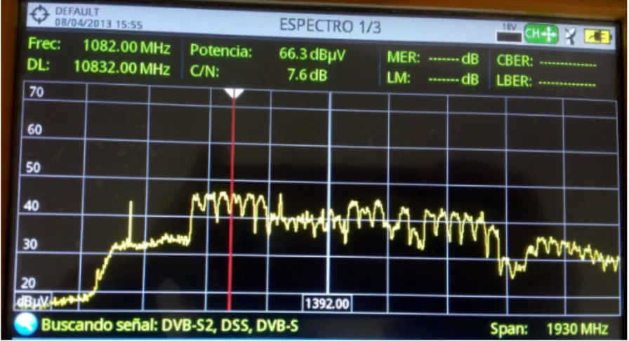
DVB-S/DVB-S2 channels (transponders) have a bandwidth of approximately 27 MHz with center frequency between 10.7 GHz and 12.75 GHz. The signals are transmitted using horizontal and vertical polarization. In order to use the channels that are available as

efficiently as possible, signals are transmitted at both horizontal and vertical polarization. Channels at horizontal (H) polarization are transmitted in the space between vertical (V) channels and viceversa, to avoid cross-table between channels. This implies that the satellite transmits programs (channels) in horizontal and vertical polarization, which can be observed in the spectrum. As a result, there is an alternation between vertical and horizontal channel polarization.

The digital satellite television spectrum of each channel is almost flat and TV channels are transmitted in a total band that spans around 2 GHz, as can be observed in Figure2.1.

Figure 2.1: 19.2oE ASTRA digital satellite television spectrum.

As will be mentioned in section3.3., DVB-S/DVB-S2 signals have a high range resolution due to its wide bandwidth, which makes them competitives compared to other passive radar signals. Some analysis of the properties of DVB-S signal for passive radar applica-tions is carried out in [8].

2.3.

Transmitters

The satellites who are in charge of transmitting the digital satellite television signals are located at the geostationary orbit, remaining in a fixed position relative to any ground re-ceiving location. Therefore, the receiver antenna can be pointing permanently to the the apparent fixed position of the satellite. The satellite locations are defined in longitude, since its latitude is considered null. There exist the orbital positions windows, where more than one satellite can be placed in the same longitude orbital position so that TV view-ers can receive a greater choice of programs with a fixed dish antenna. For example the position 19.2oE of ASTRA that is composed by a constellation of 4 satellites (ASTRA 1KR/1L/1M/1N).

The transmission of digital satellite television is based on using the satellite as a relay station, so the transmission is constituted by two communications links. The first one is the Up-link, where the television signal that needs to be distributed is first up-converted to a high microwave frequency and transmitted with large directive parabolic antennas (diameter from 9 m to 12 m) to the corresponding geostationary satellite.

to 12.75 GHz) of the television signal and retransmits it towards its entire coverage area. These digital satellite television signals are received by ground stations where each one has a parabolic dish (diameter from 45 cm to 120 cm) that is pointing to the geostationary satellite, a Low-Noise-Block converter (LNB) and a tuner or a decoder to watch TV.

Figure 2.2: Digital Satellite Television transmission-reception links.

2.3.1.

Choice of an opportunity transmitter

The operators of digital satellite television with the greatest presence in the region where our antennas have been installed are Hispasat and ASTRA. Therefore, it is necessary to choose between them which is the best constellation of satellites that provide us with the best direct path signal-to-noise ratio and the best pointing antenna conditions.

The 30oW Hispasat satellite constellation provides the highest EIRP, but the pointing an-tenna conditions is worth than pointing to the 19.2oE ASTRA constellation. Taking into account that the satellite signal is only received if there is line of sight (LOS), the obstacles that can have block the line of sight will be studied in each transmitter case. A precise pointing of the directive UP antenna to different constellations has been done, monitoring the RF power of the received signals with a spectrum analyzer. Hence, it has been decided to choose the 19.2oE ASTRA satellites constellation as transmitters of opportunity.

As will be discussed later, the fact of choosing this opportunity transmitter allows us to receive signals from digital satellite television with carrier-to-noise ratio above the estab-lished minimum. Also, it permits us to choose channels with different DVB-S and DVB-S2 standards (using the predefined filters of L1 and L5 of the receiving instrument) and from different transmitters (1KR and 1M). The received digital satellite television signals are transmitted by the 1KR and 1M satellites from the 19.2oE ASTRA constellation.

As following, the coverage of 19.2oE ASTRA 1KR and 1M satellites can be observed, where the transmitted EIRP in the area that covers the Institute of Space Sciences (Cer-danyola del Vall `es) is 50 dBW.

(a) 19.2oE ASTRA 1M. (b) 19.2oE ASTRA 1KR.

Figure 2.3: 19.2oE ASTRA 1KR and 1M coverage, from

The IEEE Standard 686-2008 [1] defines bistatic radar as a radio detecting ranging system that uses electromagnetic waves to detect and track targets,using antennas for transmis-sion and reception at sufficiently different locations that the angles or ranges from those locations to the target are significantly different.

Unlike classical bistatic radars, Passive Bistatic Radars (PBR) make use of transmitters of opportunity instead of a cooperative transmitter, so they are intrinsically a non-cooperative system. The target detection and the estimation of its parameters is based on a com-parison between received signals, direct signal of the transmitter of opportunity and the scattered signals.

Due to the advantage of not needing a transmitter specifically designed for PBRs and they result in cheaper systems, they have a significant attraction for the scientific-technical community and many advances are being made on these systems. Table3.1 shows the main advantages and disadvantages of the PBR systems:

Table 3.1: Advantages and Disadvantages of Passive Bistatic Radars

Advantages Disadvantages

Relatively low cost Inherent inability of the design on the

transmitter

Low vulnerability Complicated geometry compared with

monostatic radar

No demand for frequency allocation Advanced hardware and software

technology

Military applications: Some transmitter’s ambiguity functions

stealth and immune to Anti-Radiation Missiles are not proper for radar operation No jamming Reduced impact on the environment

Large number of transmitters Covert operation

High transmitters coverage

There are several types of illuminators of opportunity, such as Global Navigation Satellite Systems (GNSS), Terrestrial and Satellite Digital Television, FM radio, etc. The reason for using digital satellite TV signals is that the available power, bandwidth, number of trans-mitters and coverage is greater than in GNSS. In this chapter we will describe the basic elements of a radar which uses the transmissions of Satellite Digital Television already present in the region of interest as the radar waveform.

3.1.

Geometry definition

The bistatic geometry of the PBR system is based on the separation in distance of the transmitter and receiver. This geometry affects the performance of the system in terms of detection range and resolution.

The opportunity signals are unknown by the radar receiver, so the PBRs usually need two 9

receiving antennas. The reference receiver antenna, which is steered toward the trans-mitter of opportunity, collects the reference signal and the surveillance receiver antenna collects the signals backscattered from the pointing area. The receiving system may also consist of a single receiving antenna, with the disadvantage that the data collector system of the receiver will be more complex.

The coordinate system used to describe the geometry will be in a two dimensional situation with a north referenced coordinate system. It must be said that in the experiments carried out for this project, two receiving antennas have been used, but both are considered to be in the same geographical position due to its proximity. An illustration of a passive bistatic radar can be seen in Figure3.1.

Figure 3.1: Bistatic radar geometry (also applied for PBR).

TxandRxare the position of transmitter and receiver, respectively, being separated with a baseline direct path lineL. The distanceRT is the range from the transmitter to the target, whileRRis the range from the target to the receiver. The sum of both mentioned distances will be the distance travelled by the opportunity signal scattered on the target.

The bistatic angle (β) is one of the important parameters that characterizes the bistatic radar and affects to the system performance. It can vary between 180o when the target is on the baseline to 0o when the target is on the pseudomonostatic region, a special bistatic geometry that approximates monostatic operation or in practice it defines bistatic operation near the extended baseline. Also the transmitter and receiver looking angles, can be defined asθR andθT respectively. In addition, the target’s velocity vector projected onto the plane has magnitudeV and direction with aspect angleδ.

When omnidirectional antennas are used to receive the scattered signals, whenRT +RRis measured with bistatic configuration, the target position can be located on every point of a constant range ellipse with focal points in the transmitter and receiver. In the case studied in this project, the receiving antenna of the signals reflected in the targets is directive, so there is no uncertainty of the location of the targets.

3.2.

Radar equation

The bistatic radar equation can be used to predict the performance of the passive bistatic radars. Indeed, the quantity of interest is the power received (sensitivity) at the receiver antenna for a given geometry, target and transmitter. It is known, that the power of trans-mitted signal is expressed using theEffectiveIsotropicRadiatedPower(EIRP=PTηDT). The satellite transmitter transmits a signal of bandwidthB at wavelength λ, with a peak transmit powerPT and with an antenna of directivity DT and efficiency η. The target is located at a distanceRT from the transmitter and a distanceRR from the receiver has a bistatic radar cross sectionσ. The bistatic radar cross section, also expressed as BRCS, quantifies how detectable a target is in a bistatic configuration, expressing indirectly its equivalent size and ability to reflect the transmitted signal in the direction of the receiver compared to an isotropic reflector. The BRCS has units of area.

It is considered that the scattered signal spreads as a spherical wave and that it is inter-cepted by the receiver antenna of directivity DR and efficiency ηR. Being in a non-ideal scenario, where non free-space is assumed, we can consider a loss factorFL>1. This factor takes into account effects such as attenuation losses, interferences, diffraction, mul-tipath and other environmental factors. Concerning to the receiver system losses, a loss factor is appliedLs>1. As a result, the radar equation relationship can be developed as in equation (3.1). PR= EIRP 4πR2_Tσ ηRDR 4πR2_RLsFL λ2 4π (3.1)

The noise power at the receiver is given by3.2.

PN=kBT0BF (3.2)

WhereF is the receiver noise factor,Bis the receiver bandwidth,T0= 290 K is the

refer-ence room temperature andkB= 1.38 x10−23 W/(Hz K) is the Boltzmann’s constant.

SNRis defined as the measure of signal strength relative to the background noise. So the

SNRis computed in (3.3) as the ratio between the power received and the thermal noise power (PN) at the receiver.

SNR= PR PN = EIRPλ 2_η RDRσ (4π)3_R2 TR2RLsFL 1 kBT0BF (3.3)

3.2.1.

Pulse compression

To increase the probability of detection for a given scenario it is necessary to maximise the SNR of the target returns. So, to increase the SNR a possible solution is to integrate over time. It can only be applied if the target and receiver are stationary, in this scene the target samples add in phase.

Taking into account argumentations from [2],Bfrom (3.3) is replaced by the inverse of the coherent processing interval defined asTinc.

B= 1 Tinc

(3.4) Increasing the reflected power in the target and incoherently increasing the noise power, the resulting is an increase in the target reflected signal-to-noise ratio by a factor of10 log₁₀(Tinc) in dB. The pulse compression is equivalent to a matched filter processing.

3.3.

Range relationship

The resolution of a radar is defined as the minimum separation between point targets that allows them to be individually distinguished by radar signal processing in both range and Doppler. The bistatic range is defined as the sum of the transmitter-target range (RT) and target-receiver (RR). As has been said in Section 3.1., with a bistatic geometry the target can be located on an iso-range ellipse with focal points in the transmitter and receiver (in the case of using omnidirectional antennae). This means that the range resolution has dependence on the bistatic geometry.

Because of the bistatic radar configuration, PBR has range cells that are given by the difference of the range resolution in two concentric ellipses (Figure 3.2), so the range resolution becomes dependent of the bistatic angle (β). The range resolution of all radar systems is given by the bandwidth of the radar signal, or the opportunity signal bandwidth in case of a PBR.

Figure 3.2: Bistatic radar range resolution with an iso-range ellipse contour.

Furthermore, the bistatic range resolution,∆RB, can be approximated as in equation (3.5). It can be observed that the best case of range resolution occurs whenβ is null and the range resolution becomes minimum, with a pseudomonostatic scenario (whenTx,Rxand the target are approximately located in the baseline) and non a bistatic one. The worst case of bistatic range resolution is when it becomes maximum and that occurs when the bistatic angle approaches to 180o.

∆RB=

c

2Bcos(β/2) =

∆RM

cos(β/2) (3.5)

Where c = 299,792,458 m/s is the speed of light, B is the processed signal bandwidth and

monostatic case (transmitter and receiver are located in the same place). As can be ob-served, the range resolution depends on the bandwidth and on the bistatic configuration. With the same bistatic configuration and knowing that the bandwidth of the measured dig-ital satellite TV signal as mentioned above is larger than other illuminators of opportunity. The great advantage of digital satellite TV signals large available power and broader total bandwidth, compared with other illuminators of opportunity.

A specific calculation of the range resolution will be made for digital satellite television signals and will be compared with digital terrestrial television signals (DVB-T) and a type of GNSS signals.

The bandwidth of a DVB-S/S2 transponder can take different values, in these example a frequent value of 27 MHz is chosen. After the instrument and software processing of the signals, in our case the bandwidth of the processed signal is 20 MHz (digital filter of 10 MHz cutoff frequency in baseband is applied). In our Ground Station location, the 19.2oE ASTRA satellites have an elevation of approximately 39o, so the minimum bistatic angle isβ= 39o (when GS and target are at the same altitude). The resulting minimum range resolution with the explained configuration is∆RB= 15.91 m.

For the same bistatic angle, a DVB-T passive bistatic radar capable of selectively receive a single UHF band TV-signal channel of 8 MHz bandwidth has a range resolution of∆RB = 39.75 m. In the case of one type of GNSS at L1 (CA code), for the same bistatic angle and considering a pulse width of2µsafter correlating, the range resolution is∆RB = 318 m.

3.4.

Velocity and Doppler shift

The Doppler shift is the rate of change of the total path length of the reflected signal, normalized by the wavelength. For a bistatic radar, the Doppler shift of a reflected signal without taking into account the relativistic effects is given by (3.6).

fB= 1 λ d dt(RT +RR) (3.6) In reference to Figure3.1, it is know that the target’s velocity has magnitudeV and aspect angleδ. In the case of static transmitter and receiver, the projections of the target velocity vector will be onto the transmitter-target line of sight and onto the target-receiver line of sight.

dRT

dt =V cos(δ−β/2) (3.7)

dRT

dt =V cos(δ+β/2) (3.8)

After combining equations (3.7) and (3.8), the bistatic Doppler shift for static transmitter and receiver is described in equation (3.9).

fB= 2V

Also, the bistatic velocity or the projected target velocity can be defined as follows:

vB=V cos(δ)cos(β/2) (3.10)

fB= 2vB

λ (3.11)

In Figure3.3it is shown the normalized Doppler shift fb(cosδ,cosβ₂)as a function of the aspect angle of the target velocity vector for different bistatic angles. Can be observed that monostatic Doppler shift occurs in the case ofβ = 0oand the bistatic Doppler shift is nullified whenβ = 180o.

δ: Angle of the target velocity [º]

-180 -150 -120 -90 -60 -30 0 30 60 90 120 150 180

Normalized Doppler shift [Hz]

-1 -0.8 -0.6 -0.4 -0.2 0 0.2 0.4 0.6 0.8

1 Normalized Doppler shift as a function of δ for different β β =0 º β =30 º β =60 º β =90 º β =120 º β =150 º β =180 º

Figure 3.3: Normalized Doppler shift as a function ofδfor differentβ

3.5.

Ambiguity function

The signal processing of the proposed radars consists in cross-correlating the direct and reflected signals. This is equivalent to the matched filter processing when the SNR of the direct signal is sufficiently large [9]. The investigation of the correlation properties of the used illuminator signal is essential. In order to analyze the potential opportunities of the used illuminator signals, the ambiguity function and resultant ambiguity surface plot provide a useful tool for analysis.

The ambiguity function depends largely on the radar waveform (and in case of PBR sys-tems, on the signal of opportunity waveform), being the ability of a radar to detect targets amongst returns from other objects (clutter) in a region of interest and the ability to deter-mine parameters of these targets, such as range, bearing, size and velocity.

In general, the ambiguity function for a transmitted signal x(t) is a 2-D autocorrelation given by the following (3.12):

Rx,x(τ,fD) = Z +∞

−∞ x(t)x

∗_(t−τ)e−j2πfDt_{dt (3.12)}

Whereτand fD are the delay and doppler frequency, respectively. x(t)is the transmitted complex signal, also known as reference signal, andx∗(t)is its complex conjugate. Some properties of the ambiguity function include:

• The maximum ambiguity function value occurs at the origin, since the received sig-nal arrives with the same delay and zero Doppler shift at the receiver. Also, the maximum ambiguity function value equals to the total power of the signal (in our case it is used a digital filter that applies a unitary gain in order to not magnify the magnitude ): |Rx,x(τ,fD)|max =Rx,x(0,0) =Px.

• The ambiguity surface is symmetric along both time delay and frequency axes:

Rx,x(τ,fD) =Rx,x(−τ,fD)andRx,x(τ,fD) =Rx,x(τ,−fD).

When the spectral power density has a rectangular shape, the cross-correlation function has a sinc shape along theτdomain.

3.5.1.

Measured ambiguity function

In order to verify that digital satellite television signals are a good source of opportunity for use in passive bistatic radar systems, it has been decided to measure the ambiguity function for an specific case. Using only the UP antenna pointing to the 19.2oE ASTRA satellites (pointing angles of 155.11o azimuth and 38.97o elevation), the auto-correlation of the direct path received signal is computed by taking the channel obtained with L1 filter of the instrument. For the calculation of the ambiguity function the techniques of software signal processing have been used, which will be mentioned later in5.2..

Figure3.5.1. shows the measured ambiguity function (in Delay Doppler Map form) of the digital satellite TV signal transmitted by 1KR 19.2oE ASTRA satellite. This corresponds to the TV channel with central frequency of 11318 MHz. The lags are defined as the temporal distance between both correlated signals (distance delay), it will be explained in more detail later.

(a) Ambiguity Function from -40 Hz (freq bin 0) to 40 Hz (freq bin 81).

(b) Ambiguity Function zoomed in frequency, from -10 Hz (freq bin 0) to 10 Hz (freq bin 21).

Figure 3.4: Ambiguity function of the DVB-S/DVB-S2 signal transmitted by 19.2oE ASTRA 1KR satellite with carrier frequency fc = 11318 MHz (applying digital filtering with a 7th order Butterworth filter with cutoff frequency fc= 10 MHz).

Delay Doppler Maps (DDM) are computed using thewavpysoftware library [13]. The ”freq bin” axis is always defined between opposed frequencies, being0Hz= fmax−fmin

2 freq bin

the central frequency. Therefore, the defined axis will start at0freq bin and it will end at the(fmax−fmin+1)freq bin.

It’s been said said that the auto-correlation calculation acts as if the signal has passed through a matched filter. Taking into account this principle, the ambiguity function repre-sented in a Delay-Doppler map represents the output of a matched filter bank where it is composed of the reference signal and its Doppler shifted copies.

Figure 3.5: Lag (time delay) profile of the figure 3.4(a) and ambiguity function at 0 Hz Doppler frequency.

It can also be observed that the used illuminator signal has a good correlation properties and Doppler shifted copy of itself, only having a peak in both zero time and doppler fre-quency. In general, it can be said that a signal has advantageous correlation properties if the structure of the signal is noiselike with broadband smooth spectrum, as the digital satellite television signals. According to the ambiguity function shown before, the digital satellite TV provides appropiate signals for being used in a passive bistatic radar. There is a dynamic range enough to identify correlation peaks provoked due to some target reflec-tions.

3.6.

Direct Signal Interference

A challenge with the passive radars is to apply algorithms in order to suppress the strong direct signal incoming at the surveillance antenna (pointing to the scatterers), emitted from the transmitter, in order to be able to detect targets with weaker reflected signals. The direct signal at zero Doppler emitted from the transmitter does also leak into the secondary lobes of the antenna that points to the scatterers. This may hide weaker echoes that are below the secondary lobes of the ambiguity function.

A potential countermeasure capable of neutralizing the direct signal interference is to place a big metal shield in the direction of the transmitter. This is not possible, and there may be contributions of the direct signal from other incoming angles, caused by reflections from, e.g., nearby buildings and terrain.

A more practical solution might be to use direct signal interference mitigation techniques such as [22], [23], [24], [25] and [26]. Finally, a DSI mitigation technique of the wavpy

4.1.

Receiver instrument

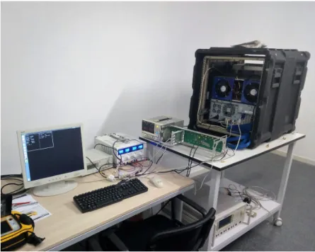
The existing receiver instrument, called BIBA-SPIR (Bi-Band Software PARIS Interfero-metric Receiver) [12], developed by the Earth Observation research group of the Institute of Space Sciences has been used to record digital satellite television direct and reflected signals. One antenna has been used for each link. The UP antenna receives the direct signal from the transmitter satellite and the DW antenna receives the reflected signal. This instrument consists of an RF receiver with two dual-band channels (UP,DW), A/D converters and programmable local oscillator frequency and bandwidth. BIBA-SPIR is capable to manage a sustained recording data rate of 320 MB/s, with a highly accurate GPS time reference. For that a GPS antenna is used to obtain the time and positioning information.

Figure 4.1: BIBA-SPIR instrument setup.

The sampled data of the recorded signals is stored into files of 1 GPS second, where the in-phase and quadrature components of the signals are digitized with one bit per sample and are sampled at a rate of 80 Msamples/s. These generated files will be used to make the software signal post-processing in section5.2.

In Figure 4.1, it can be observed the BIBA-SPIR instrument with its corresponding RF front end, power supplies, control computer and the necessary wiring to feed the LNBs, the GPS antenna and to receive the direct and reflected digital satellite TV signals. In Figure4.2 it is shown a more detailed view of the BIBA-SPIR instrument dual band front-end (simultaneous L1 and L5 frequencies).

Figure 4.2: BIBA-SPIR front-end (image extracted from [12]).

Also a Graphical Interface User (GUI) is used to start and stop the recording, where L1-UP/DW and L5-L1-UP/DW parameters are configurable.

Figure 4.3: SPIR’s GUI with configurable parameters.

4.2.

Ground Station setup

For the accomplishment of these experiments a Ground Station (GS) has been set-up, where the assembly of the receiving antennas has been made on the roof of the Institute of Space Sciences (ICE-CSIC) building. This location provides the opportunity of easily pointing the uplink antenna (UP) that receives the ASTRA 19.2E satellite digital TV signals and the downlink antenna (DW) that receives the reflected signals. The DW antenna can be pointed into many possible scatterers as buildings, trees, cars, even planes/helicopters and rain clusters.

Figure 4.4: Explanatory diagram of the PBR setup.

As can be observed in Figure4.2., a commercial parabolic dish antenna of 60 cm diameter is used to collect the direct path signal (UP) provided by the satellite and in the focus of the dish is located an LNB (SMW PLL-LNB ext. 10 MHz refB) in charge of amplifying the signal received from the satellite, shift it to L-band and distribute it, through coaxial cable, to the BIBA-SPIR instrument.

(a) DW antenna with broader beam. (b) Directive DW antenna.

Figure 4.5: Ground Station UP and DW antennas.

An identical LNB is used for the downlink antenna (DW), employed to collect the reflected path signals. The difference with respect to the UP antenna is that in the tests realized the DW antenna was only the LNB feedhorn (without dish), and was used first to have a broader beamwidth , and later the parabolic dish was added to have more directivity and be able to have more precision pointing to the scatterers. Beamwidth of the feedhorn is

estimated to be approximately 30oand the beamwidth of the used parabolic dish antennas is approximately 4.5o.

The initial purpose of mounting this set-up on the roof of the institute building was to collect data in rain scenarios and try to detect rain clusters. Due to the fact that during the real-ization of this project there have not been events of high intensity precipitation with clouds close to our setup, signals reflected in other targets have been collected as can be seen in the experimental results in chapter6.

4.2.1.

Pointing of the UP antenna

The UP antenna has been pointed to the 19.2oE ASTRA satellites constellation, in order to receive satellite digital TV signals. For this purpose, it is necessary to find the satellite/s that provide the best coverage according to the geographical location of the Ground Station and compute the angles of azimuth and elevation required for pointing the antenna to the satellite.

Digital TV satellites are defined as geostationary with a non retrograde circular orbit in the equatorial plane (null inclination and eccentricity). These satellites theoretically remain motionless on a given point on Earth, although they have a window of motion, so they have the same angular velocity as Earth. The ground station antenna uplink (UP) an-tenna does not need adjusting, because no tracking is necessary. Therefore, the following characteristics of geostationary satellites can be defined:

Figure 4.6: Example of geostationary orbit.

Taking into account that a sidereal day is the period of the Earth rotation over its axis and its value is T = 23h 56min 4.1s = 86164.1s. In a perfect Keplerian movement with geocentric gravitational constantµ= 398600.4418 km3

s2 , the nominal orbit radiusrcan be

computed with the following equation:

T =2π

s

r3

µ (4.1)

Moreover, can be computed the satellite GEO orbital height (in this case using nominal Earth radiusRT, although in the made scripts has been computed a specific Earth radius for each Earth location).

r0=r−RT =35786.157km

The digital TV satallites that provide the best coverage in the Ground Station region are from that ones from ASTRA are situated in an orbital location of 19.2oE, as the 1M/1KR. In

order to compute the pointing angles (azimuth and elevation) of the uplink antenna, must be calculated the distance between the Ground Station and the chosen satellite using the Earth-Centered-Earth-Fixed (ECEF) reference system.

The location of the Ground Station is obtained from a GPS receiver, so it was defined in geographical coordinates: Latitude, Longitude and Altitude. The location of the satellite it is also in the same reference system, but for simplifying the calculations a reference system change is made to ECEF.

UsingWorldGeodeticSystem84Earth model with semimajor axisa=6378137mand ec-centricitye=0.0818, the prime vertical radius of curvature (N) and the ECEF coordinates (x,y,z) can be defined. N=q a 1−e2_sin2_(φ) (4.2) x= (N+h)cos(φ)cos(λ) (4.3) y= (N+h)cos(φ)sin(λ) (4.4) z= ((1−e2)N+h)sin(φ) (4.5)

Whereφ,λandhare the latitude, longitude and altitude, respectively.

Table 4.1: Geographical locations.

Latitude [o] Longitude [o] Altitude [m] Ground Station 41.500436 2.110422 138 ASTRA 1M/KR 0.000000 19.200000 35,786,000

Figure 4.7: Pointing Angles of the Uplink antenna

Knowing the value of the latitude of the Ground Station (φGS) and the relative satellite longitude (λsat), the pointing angles azimuth and elevation can be computed.

α=tg−1 tan(λsat) sin(φGS) (4.6) The azimuth (α) is the angle between the ground station meridian and the local verti-cal plane that contains the satellite pointing direction. It is measured from the North and ranges from 0o to 360o. The azimuth angle computation varies depending on the geo-graphical situation of the Ground Station:

North - West: A= 180o-α

North - East: A= 180o+α

South - West: A=α

South - East: A= 360o-α

The elevation (ε) is the angle between the satellite pointing direction and the local horizon of the Ground Station.

ε= cos(λsat)cos(φGS)−

RT RT+R0 p 1−cos2_(λ sat)cos2(φGS) (4.7)

Table 4.2: UP antenna pointing angles and distance to satellites. GS - 1M distance [m] UP true azimuth [o] UP true elevation [o]

37,851,814.71 155.11 38.97

4.2.2.

Pointing of the DW antenna

The directive DW antenna must be used when it is necessary to perform a precise pointing towards the target. To calculate the pointing angles of the DW antenna, the first step is to know the geographical coordinates (φ,λandh) of the Ground Station and of each target.

The purpose is to convert the direction vector (ρ¯ =r¯−_R¯_{vector between Ground Station} and target) in ECEF coordinates to Azimuth and Elevation given geocentric latitude, east longitude, and height above the ellipsoid of the Ground Station.

A reference system must be created at the point where the pointing is performed, so the reference system (Antenna-Centered-Antenna-Fixed) is created with origin in the Ground Station. In the ACAF reference system there are three unitary axis: Sˆ (pointing to the South) ,Eˆ (pointing to the East),Sˆ(pointing to the Zenith).

Figure 4.9: ACAF reference system, based on images of [6].

A rotation matrix is calculated in order to make base changes between the ECEF and ACAF reference systems.

  ˆ S ˙ E ˙ Z  =  

sin(φGS)cos(λGS) sin(φGS)sin(λGS) −cos(φGS)

−sin(λGS) cos(λGS) 0

cos(φ_GS)cos(λ_GS) cos(φ_GS)cos(λ_GS) sin(φ_GS)

    ˆ i ˆ j ˆ k   (4.8)

In order to getS,EandZ, the ECEF coordinates (x,y,z) of the direction vectorρ¯have been replaced in the transposed vector[ˆ_i,jˆ_,kˆ_{]. Therefore, the direction vector is transformed to} the ACAF reference system:ρ¯ =SSˆ+EEˆ+ZZˆ.

S=−ρcos(E)cos(A) (4.9)

E=ρcos(E)sin(A) (4.10)

Z=ρsin(E) (4.11)

The elevation (ε) and azimuth (α) can be computed. The functionatan2(y,x)is the arctan-gent function with two arguments, giving the angle between the positive x-axis of a plane and the point given by the coordinates (x, y) on it. This function returns the appropriate quadrant of the computed angle.

ε=sin−1 Z ρ ,−90o≤ε≤90o (4.12) α=atan2(E,−S),0≤α≤360o (4.13)

5.1.

Instrument processing

In this section, the signal processing performed by the instrument will be explained briefly. It is known that the frequency band of digital satellite television is between 10.7 and 12.75 GHz approximately. So, the LNB usedBis in charge of performing a frequency band con-version with a local oscillator whose value has been previously chosen for the low band (fLOX = 9.75 GHz) so that the signals can be transmitted by the coaxial cables. Then, the

BIBA-SPIR proceeds to filter the received signals, with a 40 MHz filter at L-band, and shifts the signals to baseband (applying a local oscillator programming frequency equals to fLOL₁

= 1575.0 MHz or fLOL₅ = 1176.25 MHz). Finally, the signals are I/Q (In-phase/Quadrature)

sampled with 4 bits/sample and a sampling rate of 80 Msamples/second. In Figure5.1it can be observed the block diagram of the BIBA-SPIR and in Figure5.2a graphic explana-tion of the instrument processing is shown.

Figure 5.1: Dual-band SPIR (BIBA-SPIR) block diagram, having [12] as reference.

Figure 5.2: Spectrum frequency translation during instrument processing (not in scale). 27

5.2.

Software post-processing

In this section the post-processing techniques that have been applied to the BIBA-SPIR raw data in order to obtain several waveforms will be explained. This signal post-processing has been applied off-line using an open source C++/Fortran90 software library for GNSS-R data analysis and modelling: wavpy[13]. Some contributions have been made to this library, that will be detailed in section5.2.3.

The main objective of applying signal processing is to make an instrumental calibration and generate the pulse compression. Figure 5.3 shows a block diagram of the software post-processing of the recorded signals.

Figure 5.3: Software processing block diagram.

The first step in the processing of the recorded signals is to calibrate the instrumental DC offset originated at the ADC converters. Next, the television channel of the direct signal from which the most power has been received is chosen (depending on the L1 / L5 band and the polarization of the LNB), and the spectrum of the direct and reflected signals is shifted to the base-band by locating the carrier frequency of the channel selected at 0 frequency. Lastly, a digital filter is applied to obtain the selected television channel. This filter is applied in both direct and reflected signals.

The direct and reflected complex signals can be expressed as in equations (5.1) and (5.2).

sU P(t) =s(t−TU P) =A(t−TU P)ej2πfc(t−TU P) (5.1)

sDW(t) =s(t−TDW) =A(t−TDW)ej2πfc(t−TDW) (5.2) Wheres(t)is the signal transmitted by the satellite, Ais its envelope, fc is its carrier fre-quency andTU PandTDW are the time of propagation of the transmitted signal in the direct and reflected path, respectively. Therefore, the complex signals can also be expressed using the in-phase (real) and quadrature (imaginary) components of analytic signals.

sDW(t) =iDW(t) +qsDW(t) (5.4)

5.2.1.

Correlation

The cross-correlation is defined as a measure of similarity of two signals as a function of its relative displacement. The auto-correlation is the cross-correlation of a signal with itself. The autocorrelation at the origin is always maximum and equals the power of the signal. In the case of our PBR system, it is desired to determine the bistatic range of the target measuring the time difference (delay) of arrival of the reflected signal respect to the direct signal. The time difference between the reflected signalsDW and the direct path signalsU P can be calculated by cross-correlating these signals. Therefore, the cross-correlation of direct and reflected signals for continuous and discrete time can be computed as (5.5) and (5.6), respectively, in the case of fixed transmitter and receiver antennas and ignoring the effects of moving scatterers (without Doppler).

RDW,U P(t0,τ) = 1 T Z t0+T t0 sDW(t)sU P∗ (t−τ)dt (5.5)

The asterisk ins_{U P}∗ denotes the complex conjugate of the signal. The variableτis defined as the relative temporal delay applied to the signals. In the signal processing theory, the correlation of two signals is done during an integration time T, in our case we also specify the initial time (t0) at which the correlation integral is computed. So, we select a segment

of the signal of duration T that starts at t0. When the computation result of the

cross-correlation results in a peak, it corresponds to the bistatic time delay.

In practical cases where a receiver device is used, as the BIBA-SPIR receiver in our case, the signals are sampled with a sampling frequency rate fs. Consequently, the correlation must be computed in discrete-time.

RDW,U P(t0,τ) t=n/fs =RDW,U P[n0,m] = 1 N n0+N−1

∑

The computation of cross-correlation of two signals is carried out in the time domain, using thewavpy[13] software library. Referring to equation (5.6): Nis the number of samples to be integred,n0is the initial sample at which the correlation integral is computed andm

is the lag number. The output of the cross-correlation computation will result in a complex waveform.

The software range resolution is defined as the lag separation correspondence in distance, in the best case of approximately 3.7474 m, using equation (5.8). This means that if the lag separation is defined as 1 sample, each lag corresponds to approximately 3.7474 m difference distance between UP and DW signals.

lagseparation = c fs (5.7) = 299,792,458m/s 80∗106_sample/s =3.7474 m sample

5.2.2.

DC offset Calibration

The analytic complex signals received by the direct pathsU P(t)and the reflected sDW(t) at the input of the digital signal processor have real (in-phase) and imaginary (quadrature) components. In an ideal case, the signalssU P(t)andsDW(t)are zero mean, but in a real case there are DC offsets added to the signal as can be seen in equations (5.8) and (5.9).

sm_{U P}(t) =sU P(t) +Ko f f set (5.8)

sm_DW(t) =sU P(t) +Go f f set (5.9)

s_{U P}m (t)andsm_DW(t)are the measured signals with an added DC offset. These DC offsets are due to residual components of the noise or instrumental non-linearities (e.g., non-ideal AD converters). In order to make a DC offset cancellation, it is necessary to estimate the average value of these offsets.

Ko f f set≈K˜o f f set= 1 T Z T 0 s_{U P}m (t)dt (5.10) Go f f set ≈G˜o f f set= 1 T Z T 0 sm_DW(t)dt (5.11)

After computing the approximate values of the DC offset for each signal, they will be sub-tracted from the measured signals in order to have the ideal and zero mean signals. If the correlation had been calculated without subtracting the DC offset, this would have masked low power signals after cross-correlation.

Rm_{DW,U P}(τ) = 1 T Z T 0 s_DWm (t)s_{U P}m∗(t−τ)dt = 1 T Z T 0 sDW(t) +Ko f f set sU P∗ (t−τ) +G∗o f f set dt = 1 T Z _T 0 sDW(t)sU P∗ (t−τ)dt+ Z T 0 sDW(t)G∗o f f setdt+ + Z T 0 s_{U P}∗ (t−τ)Ko f f setdt+ Z T 0 Ko f f setG∗o f f setdt ≈ T is long enough 1 T     Z T 0 sDW(t)s∗U P(t−τ)dt+ Z T 0 Ko f f setG∗o f f setdt | {z }

offset after cross-correlation    (5.12)

5.2.3.

Filtering

The main function of a filter is to remove unwanted parts of signals, like random noise, or to extract useful parts, such signal components lying within a certain frequency band. In this project, it is desired to implement a filter to extract the maximum possible bandwidth

of a television channel, in order to have a flat spectrum. In this way, we obtain a narrow ambiguity function that is adequate for radar applications.

In the instrument, the analog input signals are sampled and digitalised using analog-to-digital converters, resulting in binary numbers of sampled values of the input signals. In order to perform the signal processing of the sampled signals through software, digital filters will be applied. Some advantages of digital filters over analog filters are listed below:

• Digital filters are programmable, so can be easily modified leaving the hardware unchanged. This flexibility can be exploited on general use computers.

• Digital filters are more stable in terms of time, temperature, humidity. Analog filters are more likely to fail and error, due to the dependency of temperature (particularly if they have active components) and the degradation in time.

• Are not subject to non-linearities (when quantization effects can be disregarded), unlike analog filters.

• When they are software implemented, they can have a high versatility to process signals in a variety of ways, including the ability to be adapted to the changes of input signals.

The main contribution made by me in the librarywavpy[13] has been a new class in C++ calledfilterD.1.1.2., in order to create and define digital filters. Also, filtering functions

(FilteringSignal) D.1.1.3. have been added in the existing classcomplex signal to

filter the received signals sampled by BIBA-SPIR instrument.

5.2.3.1. Design

Digital filters can be classified according to the necessary data that they need to compute the output. A non-recursive filter, calculates the current output from the current and the previous input values. However, a recursive filter uses previous output values, in addition to input values.

An alternative terminology on filter classification can be done according to the filter im-pulse response. The imim-pulse response of a digital filter is the output sequence from the filter when an unit impulse (sequence consisting of a single value of 1 at sampling time 0 and followed by zeros in all the remaining instants) is applied at its input. If the impulse response of the filter falls to zero after a finite time, it is known as the Finite Impulse Re-sponse (FIR) filter. However, if the impulse reRe-sponse exists indefinitely, it will be known as the Infinite Impulse Response (IIR) filter. Likewise, a recursive filter is known as an IIR filter and a non-recursive filter is known as a FIR filter. We can also have filter with recursive and non-recursive terms simultaneously.

The Fourier Transform of the impulse response of a filter (Figure 5.4) is known as the frequency response of a filter, which tells what the filter output will be (filter and phase gain) at different frequencies.

Figure 5.4: Impulse and Frequency response of a filter, from [5]

Recursive filters require more calculations to be performed, since there are previous output terms as well as input terms in the filter expression, as will be seen in Section5.2.3.2.. Nevertheless, to achieve a given frequency response characteristic using a recursive filter generally requires a much lower order filter and therefore fewer terms to be evaluated by the processor than the equivalent non-recursive filter. Overall, with recursive IIR filters, we can generally achieve a desired frequency response characteristic with a filter of lower order than for a non-recursive filter.

Therefore, if IIR recursive filters are implemented, accuracy errors are reduced because of high orders aren’t implemented. It must be said that in practical applications, the stable impulse response of the IIR filters decays to near zero in a finite number of samples. In the experiment carried out, the signals that must be filtered have been previously shifted towards the baseband frequency and subsequently the nearest and with greater amplitude television channel has been centered at the frequency 0 Hz. Then, to extract the selected TV channel a low-pass filter has been applied. The frequency response for the most com-mon IIR filters with the approximation improving as order increases are shown in Figure 5.5.

Figure 5.5: Frequency response of common IIR Low Pass Filters, from [5]

For our application, we want a flat amplitude response and near linear phase within the pass-band. In this way, the television channel is wanted to be taken as entirely as possible,