DEPARTMENT OF ECONOMICS
WORKING PAPER SERIES
20
10-02
McMASTER UNIVERSITY
Department of Economics
Kenneth Taylor Hall 426
1280 Main Street West
Hamilton, Ontario, Canada
L8S 4M4
The Effects of School Board Consolidation and Financing on Student Performance
John Leach, A. Abigail Payne, and Steve Chan* January 2010
Abstract: Over the last 20 years, states and provinces have become increasingly involved in the
financing and administration of elementary and secondary education. Local school boards, however, still retain control over key aspects of the provision of education. Historically, these boards were organized at the community level so as to meet the wants of the local community. Today, states and provinces have become more interested in consolidating school boards and moving to a more centralized funding scheme. Do these changes result in improved student achievement? This paper attempts to answer these questions by examining the school board consolidation and funding changes instituted by the province of Ontario. We differentiate the effects of the policy changes based on observed differences in the school boards prior to consolidation. We show that students in previously high wealth school boards perform worse after the policy change compared to students in previously low wealth school boards.
* Leach: Department of Economics, McMaster University, KTH 426, Hamilton, ON L8S 4M4 Canada
(email:[email protected]); Payne: Department of Economics, McMaster University, KTH 426, Hamilton, ON L8S 4M4 Canada (email: [email protected]); Chan: (email:[email protected]). This research was supported by grants from the Social
Sciences and Humanities Research Council of Canada, the Canada Foundation for Innovation, and the Ontario Innovation Trust.
We thank Tom Lemieux, Bill Duncombe Amy Schwartz, Meta Brown for comments on previous drafts. We also thank participants of the American Education Finance Association, Canadian
1. Introduction
The involvement of states and provinces in the financing of elementary and secondary
education has risen steadily over the last twenty years. A number of states and provinces now provide complete funding. Despite their increasingly large financial stakes in the school system, state-level governments have largely refrained from attempts to influence the size of school boards.1 Some of these governments encourage consolidation through separate aid programs that fund buildings and transportation (Gold, Smith and Lawton, 1995), and some governments inhibit consolidation by providing extra funding to boards that contain small and sparsely attended schools.2 However, the schools have remained under the control of school boards, and the school boards themselves have generally been free to adjust their boundaries in cooperation with other school boards. A major form of adjustment is school board consolidation.
The economic impact of consolidation is unclear. On the one hand, consolidation promotes economies of scale and scope (Micelli, 1993). A bigger school board reduces administrative costs because the size of the administrative staff rises less than proportionately with the size of the board. Larger boards are able to negotiate better prices for supplies and materials. They are also better able to utilize specialized labour such as math and science teachers, and specialized facilities such as computer labs (Andrews, Duncombe and Yinger, 2002; Dodson and Garrett, 2004).
On the other hand, consolidation reduces competition among school boards. The consolidated board has greater market power than any of the boards from which it was created. It can exercise its market power by being less creative in designing programs that draw new students, or by being less attentive to cost control. A bigger school board might also be less accountable to the community that it serves, which could be a serious problem in a socially diverse community. Although the impact of reduced competition across school boards is at least partially offset by greater competition among
1 The term “school boards” is analogous to the US term “school districts.”
schools, Urquiola (2005) argues that competition occurs mainly among the boards. He also argues that too little is known about its impact to draw broad conclusions about the economic impact of
consolidation.3
The empirical research on the link between consolidation and student performance is limited, but research into two related issues provides some guidance. The first issue is the measurement of the economies of scale and scope experienced by large schools. Duncombe et al. (1995) finds that school boards with moderate enrollments have lower operating costs than those with very low enrollments, but that there are diseconomies of scale in boards with more than 5,000 students. Brasington (1999)
examines the impact of board-initiated consolidations upon operating costs. However, inferring
economies of scale from cross-sectional data on operating costs is somewhat problematic. A board can respond to economies of scale by reducing taxes that it levies on its supporters or by expanding its services to students. If the board reduces taxes, the operating costs are an accurate reflection of
economies of scale, but the economies of scale are not likely to lead to better student performance. If it provides better services, the economies of scale are likely to lead to better student performance but are not accurately measured by operating costs. Gordon and Knight (2008) address the cross-sectional problem by studying the merger of small school districts in Iowa in the 1990s. They fail to find strong effects of the consolidation on outcomes such as pupil-teacher ratios, enrollments, revenues, and expenditures. In all of these studies, there is a further estimation issue. Namely, there is a selection problem if there are systematic differences in the social or economic environments in which the various schools operate, so that there is variation in the economies generated by consolidation. The boards that have already consolidated are the ones for whom these economies were greatest, so a cross-sectional analysis overstates the benefit of further consolidations.
The second issue is the relationship between student performance and school or school board size. Some researchers have approached this issue by regressing a test measure on school or school
board size (Driscoll, Halcoussis and Svorny, 2003; Harin and Brasington, 1996). Brasington (1997) takes this approach one step further. Using grade nine proficiency tests as a measure of performance, Brasington found that building enrollment, board enrollment and the number of high schools in a board were all negatively correlated with student performance.4 His findings are consistent with those of previous studies (Jewell, 1989; Fowler and Walberg, 1991). These papers are also subject to the endogeneity and selection problems outlined above, so one should be wary of using their results to predict the effects of further consolidation.
This paper studies an instance of consolidation that avoids the selection problem. In 1998 the newly elected government of the province of Ontario ordered widespread consolidation within the province’s public school system. Only seven of the province’s 62 English-language non-rural public school boards were not involved in a merger. These seven boards already had reasonably high enrollments.5 The consolidation was accompanied by a move to full provincial funding of school boards, so the endogeneity problem described earlier is largely avoided. The replacement of partial provincial funding with full provincial funding causes redistribution from rich boards to poor boards, however, and the effects of the redistribution is a focal point of the paper.
Section 2 discusses the 1998 Ontario reforms in more detail. Section 3 sets out a theoretical framework that guides the empirical analysis. Section 4 describes the data set and outlines the research questions. Section 5 presents the analysis, and Section 6 summarizes the findings.
2. The Reforms
Voters in Ontario elected a new leader, a Progressive Conservative, in 1995. The government’s mandate was to “re-invent the way the Ontario government works”. A major reform to the publicly
4 Brasington also found that the graduation rate increased with board size and the number of high schools in the board, but
he explains this result in terms of central cities bias. This bias would occur if, for example, central city school boards consciously chose to graduate many students that suburban and metropolitan boards would not.
5 The seven districts and there total enrollments at the time of consolidation are as follows: Lakehead (17,200), Durham
funded, non-sectarian, English-language school system6 followed in 1998. It was one of a number of major changes to social policy.7
Appendix 1 provides a detailed description of the 1998 consolidation and other educational reforms. There were two major components. The first was that the province ordered and directed widespread consolidation. Unlike most of the consolidations that have been studied, individuals could not vote on consolidation and school boards could not reject consolidation. Summary statistics for the school boards before and after consolidation are reported in Table 1. In the English speaking non-rural public school system, 62 school boards were consolidated into 25 boards. Seven boards were not involved in a consolidation. Ten of the new boards resulted from the consolidation of just two boards. The remaining eight boards resulted from the consolidation of three, four, or six boards. For the most part, the number of schools remained the same as did the average enrollment per school. There have been school closures and school openings since consolidation, but they seem to have been precipitated by changes in neighborhood demographics. There is no other discernable pattern in these events. The intent of the reform seems to have been bigger school boards rather than bigger schools.
The second major change concerned the funding of school boards. Prior to 1998 the school boards were free to set their own property tax rates, and to retain the property tax revenues for their own use. Residents and businesses were able to assign their property taxes to one of three systems: the public school boards (non-sectarian but traditionally Protestant), the Roman Catholic (or separate) school boards, or the francophone school boards (which could be public or separate). Although the province provided financial support to school boards that were unable to achieve a minimal level of spending per student (through a provincial equalization grant), these funding rules gave rise to
6 There are four publicly funded school systems in Ontario. The systems are based on home language (English or French)
and religion (Catholic or all others). In the English-language system, the consolidation affected mostly the non-sectarian boards. Very few of the Catholic (or Separate) school boards were consolidated in 1998.
7 Income and other taxes were cut, welfare spending was cut, regulations concerning who was eligible for social assistance
were changed, new social assistance programs based on the concept of workfare were created, laws concerning
discrimination were repealed or modified, changes in the rights of unions concerning worker replacement were changed, health services were restructured, and cities were amalgamated. For a detailed report of the effect of this change in the
significant variation in school board spending. For example, in 1994, the year before the election, average per student spending for the school boards that were consolidated into non-rural boards was $5,943, ranging from $4,863 to $8,125. The average provincial equalization grant was $2,813, ranging ranging -$598 to $7,015. The school boards also varied in their reliance on residential or business property taxes. The average reliance on business property taxes was 34 percent, ranging from 10 to 63 percent.
The 1998 reforms required the province to set one residential property tax rate for education and implemented a new property assessment procedure. A phased-in program to harmonize business
property taxes across the province was established. Although residents could still choose the system that would receive their tax dollars, businesses could no longer do so. Moreover, the province began to collect the revenue and distribute it to the school boards. Each board’s funding is now determined by a funding formula that takes into account the board’s enrollment, capital needs, special student needs, and a few other things. Local boards, once allocated their budget, still retain discretion with respect to the funding of each school. There is no requirement that a board follow the same formula used by the province in making its allocations. Local boards are allowed to raise additional revenue only in a very limited number of ways (for example, fundraisers and vending machine sales). There is anecdotal evidence that individual schools use the same methods to obtain additional funds.
These reforms are of interest for three reasons. First, the selection problem described above is largely avoided, because consolidation was imposed upon the school boards rather than chosen by them. Furthermore, roughly 90% of the non-rural boards in the public English-language system were involved in the consolidations, leaving little scope for selection bias. Second, a move from a funding scheme that allows school boards to determine their own funding to one that largely dictates their funding is likely to have effects on student performance. In a homogeneous society these effects are likely to arise from a weakening of inter-board competition. However, there are further effects in a heterogeneous society because communities differ in their demand for educational spending. Full
funding essentially replaces consumer sovereignty with a government dictate. The reforms provide some evidence on the impact of full funding in a heterogeneous society. Third, empirical research into consolidation is often hampered by the small number of available observations. The scope of the Ontario reforms gives rise to an unusually large data set.
3. A Model of Consolidation
The model set out below assumes that the underlying heterogeneity arises from differences in income. Suppose that each school board initially contains one school, and that the school is financed by taxing a group of identical households. Each household has one student. Each household’s
consumption is c and its income, net of all taxes except school taxes, is y. The household budget
constraint states that this income is divided between consumption and the tax levied by the school board.
y = c +
The quality of the education offered by the school depends upon e, which is the extent to which
expenditure per student exceeds certain fixed costs z: e z
The household’s welfare is an increasing and concave function of e (as a proxy for the quality of
education) and c:
( , ) ( , - - )
U u e c u e y e z
The board sets the tax to maximize the household’s welfare, implying ( - ) , 0 ' 1
e y z
Equivalently,
( - ) y z z
Household income does not vary within a school board, but it does vary between school boards. The optimal tax and quality of education rises with income. Assume that the income in each of the original
school boards is either high (yH) or low (yL), and let τH and τL be the optimal pre-consolidation taxes for high and low income households.
School board consolidation is assumed to take the following form.
1. Each new school board consists of two of the original schools.
2. The government sets a single tax rate t, and from the revenue collected, the
government pays each school board a per student transfer τ* such that *
L
3. The new school boards must balance their budgets, in the sense that total
spending at its schools is equal to its total transfer.
4. The per student fixed cost falls by Δz as a result of administrative economies of
scale.
The consolidated boards contain two high income schools, two low income schools, or one high and one low income school. The impact of consolidation varies across these three kinds of school board. Assuming that the board provides each school with the same per capita funding, the change in the measure of educational quality in homogeneous school boards is
, ,
i i
e z H L
The change is unambiguously positive in low income school boards, who benefit from both the
reduction in fixed costs and the redistribution of income. The change can go either way in high income school boards because the cost reduction and the redistributive effect are in opposition. Consolidation equalizes the quality of education across homogeneous school boards. Quality rises in each school board if τ* exceeds τH –Δz; otherwise, quality rises in low-income boards and falls in high income
boards.
The impact of consolidation on heterogeneous school boards in less clear because the boards control the way in which the funds are divided between the schools. A heterogeneous school board gains from consolidation (in the sense of loosening its resource constraint) only if
2
H L z
If this condition is not satisfied, consolidation must cause quality to decline in at least one of the schools in the board. If this condition is met, and if the board decides to divide the gains equally between the two schools, quality will rise at both schools but the difference in quality will (by
assumption) remain the same. However, there are other possibilities. The school board might choose to reduce the disparity by allocating the bulk of the gain to the low income school. Alternatively, if high income parents are more likely to lobby the school board or to become school board members, the greater part of the gain might be allocated to the high income school, causing disparity within the school board to rise.
The model predicts that two factors influence the impact of the reforms on student performance: the variation of household income across the pre-consolidation school boards, and the heterogeneity of the new boards. These hypotheses will be tested below.
4. The Data and the Empirical Framework
The measures used in our analysis come from school and student level data obtained under freedom of information requests from Ontario’s Ministry of Education and census data from Statistics Canada. For each publicly funded school we know the board to which a school belongs (pre and post consolidation), enrollments by grade, location of the school, and measures that capture information about the teaching and administrative staff of the schools.
For each school we know the school’s postal code. Using the first three characters of this postal code, we can identify the “forward sortation area” (FSA) to which the school belongs. An FSA is representative of the neighbourhood from which a school draws its students. The census measures are for an FSA and are gathered every 5 years (1996, 2001, etc.). We use a linear interpolation of the census measures to create annual values of the neighbourhood characteristics.
Household income was used in the model as a measure of the household’s ability to invest in education. Prior to 1998 a school board’s spending was primarily determined by its ability to tax
residential and business property.8 We use an index of property wealth to proxy ability to invest in education, or equivalently, of income (in the sense of the model). Two indices are used, one based on total property wealth and one based on residential wealth. These indices are from the final report issued by the Ontario School Board Reduction Task Force (Ontario 2006). The index is calculated as the board equalized assessment per pupil divided by the provincial average equalized assessment. Thus, if a board is at the average wealth for the province, its index would equal 1. The first index captures the wealth accessible to a board based on residential, commercial, and industrial property wealth (total wealth). The second index captures the school board’s residential tax base. Residential wealth reflects parental valuation of the neighborhoods in which they live. If, however, the parents also live in an area with a strong commercial tax base, they may also benefit from having a better endowed school system. The correlation between the two indices is 0.80.9
The indices are used to develop a discrete measure that identifies a board as being high or low income. A board is identified as “high income” under a given proxy if it is contained in the right tail of the distribution for the proxy. Figure 1 illustrates the distribution of pre-consolidation boards based on the total and residential wealth indices. Under the total wealth proxy, boards with an index greater than 1.0 (on a scale of 0.35 to 2.1) are deemed to be high income; and under the residential wealth proxy, boards with an index greater than 0.90 (on a scale of 0.35 to 2.1) are deemed to be high income. As these cut offs are somewhat arbitrary, we tested the sensitivity of these cutoffs based in our analysis by varying the cutoffs. We did not discern any significant differences in the results using different cutoffs. To further test the robustness of our results, however, we also report the results using a continuous wealth measure.
8 The province set a floor for the expected property tax revenue to be raised by a board, but boards could set a higher tax
rate. The province provided additional support only to boards whose revenues from property taxation were deemed to be insufficient.
9 We also considered an income proxy based upon the amount by which spending per student exceeded the province’s
expectations in 1994. Spending per student, averaged across all of the boards, exceeded the expected expenditure by approximately $1000. However, the excess varied across boards from almost nothing to more than $2500. Our concern with this measure is that we did not have sufficient information to understand why there was so much variation in spending across the boards, and whether this variation was only in current spending or reflected maintenance and capital
Of the 62 pre-consolidated boards, ten are categorized as high income under the total property wealth proxy and twenty are categorized as high income under the residential property wealth proxy. The six boards that were consolidated into the Toronto Board in 1998 are shown as a single point in Figure 1. These boards were sharing resources prior to the reforms, so information is not available on the wealth of these individual boards. Six boards (including the composite Toronto board) are classified as high income under both indices. Of these boards, three were part of a consolidation and three were not consolidated.
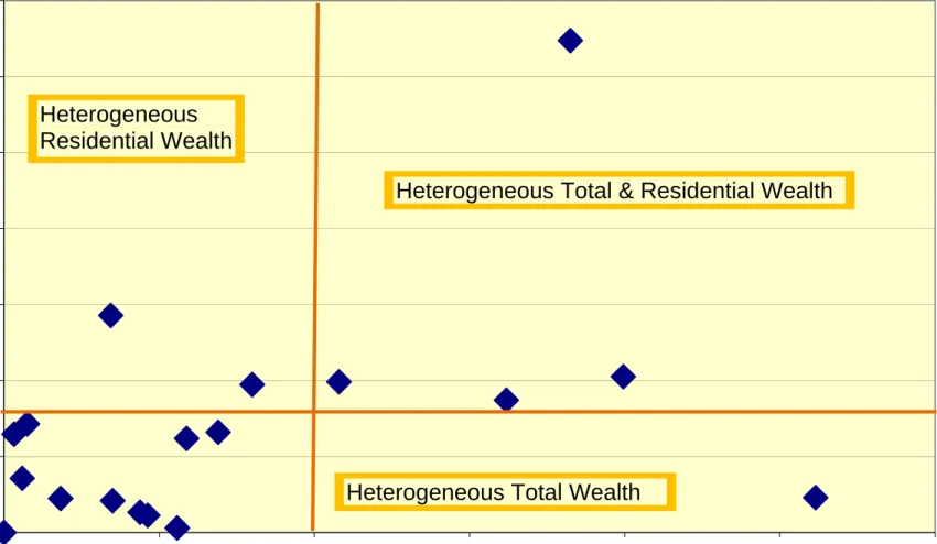
New school boards are categorized as homogeneous or heterogeneous by examining the wealth indices of the pre-consolidation boards that formed it. If the difference between the largest and smallest indices is greater than 0.40 for total wealth or 0.35 for residential wealth, the new board is said to be heterogeneous. Figure 2 shows the classification of the new boards as heterogeneous or homogeneous for both indices. Four boards are identified as heterogeneous under both of the indices. Two boards are identified as heterogeneous under the residential wealth index but homogenous under the total wealth index. One board is identified as heterogeneous under the total wealth index but homogeneous under the residential wealth index. Although there are significant differences in the way that the two indices identify high income pre-consolidation boards, the indices are quite consistent in their identification of heterogeneous new boards. They agree in all but three of the 25 cases.
Starting in 1998, Ontario instituted province-wide exams for students in grades 3, 6, and 9 as a measure of student performance within the province. Each student was expected to write exams in mathematics, reading and writing. The dependent variable in our regression analysis is the student’s average score on the three exams. The data are available from 1998 to 2004. Each student’s school and post-consolidation school board are known, as are a number of the student’s characteristics.
Only students who wrote all three exams are included in the data set.10 An exam score in each
subject ranges from 1 to 4, with higher values representing higher achievement. Panel A of Table 2 reports the average test scores for the students studied. There are test scores for 516,776 grade 3 students attending 2,257 schools. Their average score on the test was 2.67 with a standard deviation of 0.6. An average of 13 percent of the students at each school did not write all three exams; of the students with missing test scores, an average of 17 percent of these students were identified as exceptional.
We study 564,933 grade 6 students. The average performance on the test is 2.64 with a standard deviation of 0.7. An average of 11 percent of the students at each school have missing test scores; and of these students, an average of 23 percent of these students were identified as exceptional.
The basic specification of the regression equation is:
ijbt bt ijbt jbt jbt ijbt
Test Consolidation Stud School Neigh
where Test is the average test score for reading, writing, and math for student i, in grade 3 or 6, in year t. The student attends school j, which will be part of school board b after the consolidation.
Consolidation is the share of years for which a student was taught in a post-consolidation school
board. We would like to have observations on students that were never exposed to a post-consolidation school board, but since the tests were first administered in 1998, there are no such students. Instead, we have observations on students who were exposed to the post-consolidation school boards for varying lengths of time. Students who were in grade 3 in 1998 had one-third of their schooling (counting from grade 1) in the post-consolidation environment. For these students, the value assigned to Consolidation is 1/3. Students who were in grade 3 in 1999 had two-thirds of their schooling in the
post-consolidation environment and are assigned a Consolidation value of 2/3, and so on. For students
in grade 6, the consolidation measure is denominated in sixths. The consolidation measure is
interacted with measures to identify the type of board in which a student’s school is located.
Stud contains the characteristics of the test taker. It indicates whether the student is female,
a Second Language program, whether the student has been identified as exceptional (special needs), whether the student has been identified as gifted, whether the student attended kindergarten, whether the kindergarten attendance information is missing, and whether the student is enrolled in a French Immersion program. Panel B of Table 3 reports the average characteristics of the test takers. For both grades, approximately 50 percent of the test takers are female. There is no gender information for one percent of the test takers. Approximately five percent of the grade 3 and three percent of the grade 6 test takers are enrolled in English as a Second language program. Approximately two percent of the grade 3 and six percent of the grade 6 students are identified as exceptional students. An average of one percent of the grade 3 and two percent of the grade 6 students are identified as gifted students. For both grades, an average of 89 percent of the students attended kindergarten with four percent of the students having missing information about their kindergarten status. On average five percent of the grade 3 and seven percent of the grade 6 students are enrolled in French immersion programs.
School contains the characteristics of the school and the grade cohort of students for the test
takers. The first group of measures reflects the mean characteristics of the students who did and did not take the test for the grade under study and measures for the share of the students that are missing a test score and the share of the missing test score students that are identified as an exceptional student. The second group of measures reflects time-varying school characteristics which includes the share of new teachers at the school, the years of experience for the principal, whether the school is paired with another school (annex) and the share of enrollment for Francophone, Separate, and Private schools that share the same first three characters of the postal code as the school. Panel C of Table 3 reports the average characteristics of the school level measures. The averages across the schools are similar to those reported in Panel B. A low percentage of the students attend schools in areas with Francophone or private schools.
shares of the population aged 5-9, aged 10-14, with a university degree, with no high school diploma. It also includes the share of immigrants, the share of individuals of south-west Asian descent, East Asian descent, European descent, Catholic, no religion, religions other than Catholic or Protestant, and the share of houses from new stock.
Missing from this specification are measures that directly affect student ability and specific measures such as pupil/teacher ratios. Our analysis covers the results from specifications that include school fixed effects. The school fixed effects are designed to capture time-invariant measures. To the extent there is limited residential movement in a neighbourhood over the period under study, the school fixed effects will capture some of the differences that may exist across schools due to differences in student quality. Our results provide evidence of whether students in one area perform differently after the consolidation, relative to a set of students in another area. The purpose of this paper is to study whether the consolidation has differential effects across the areas that are delineated by the former school board catchments. Using recent data, student mobility across school boards between grades 3 and 6 appears to be around 6 percent. This observation suggests that it is unlikely that differences in measured student performance after consolidation across board types would be solely attributable to student mobility. It also suggests these differences can be attributable, at least in part, to changes in schooling policies that result from the consolidation and switch to full provincial funding.
5. Results
Consolidation Improves Test Scores
We explore three variations of the basic specification in Table 3. The first variation includes the measures discussed above and no others. These results are reported in columns (1) and (4). The
coefficients on the consolidation measures compare students who were in school boards that
consolidated with students who were not. The students in the non-consolidated school boards provide a control group for other reform measures that were implemented simultaneously, notably the switch to full funding.
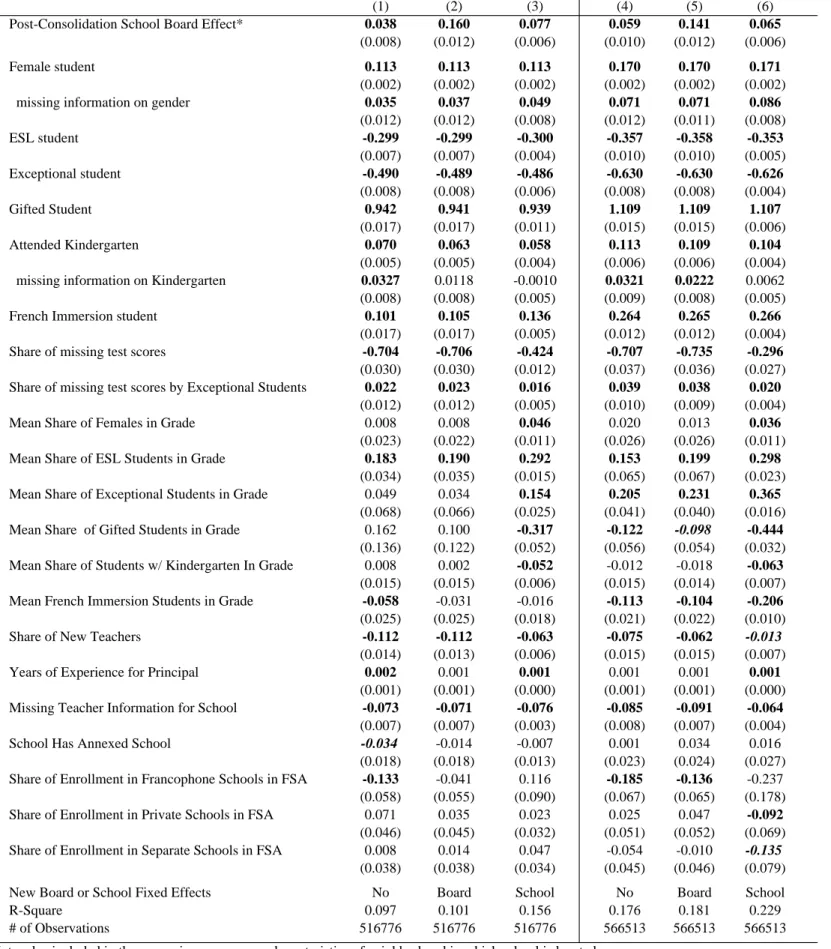
Column (1) shows the overall effect of consolidation on grade 3 test scores. Consolidation improved test scores by approximately 6 percent of a standard deviation. Also shown are the
coefficients on the student and school level measures; the signs of these coefficients are similar to those reported in other analyses. For example, girls do better than boys, ESL and exceptional students do worse, gifted students perform better, as do those students that attended kindergarten or are in a French Immersion program.
There are substantial geographic, economic, and demographic differences across the regions in Ontario, so one might expect the students at the various school boards to have different attributes that could affect their test performance. The second variation includes a set of dummies to control for any time invariant differences across the consolidated school boards. This variation estimates the effect of consolidation by comparing the performance of students that were partially affected by the
consolidation to students who were completely affected by the consolidation. The coefficients on the consolidation measure reflects the within-consolidated-board effect of the consolidation on test performance. Column (2) reports the results from the specification that includes new board fixed effects. On average the effect of consolidation within these boards is quite high. The coefficient suggests that student performance improved by 27 percent of a standard deviation after the consolidation.
Finally, the third variation includes a set of school dummies that control for any time invariant characteristics of the individual school. For example, if parents are consistently more involved with one school than another, or if a school consistently attracts a particular type of teachers, the school dummies will help control for this difference. To the extent that the regime change improved
efficiencies at the board level, one might expect the savings from the efficiencies to flow to the school, enabling the schools to deliver a higher quality of education. The coefficients on the consolidation measure reflects the within-school effect on test performance of exposure to the post-consolidation
modest 13 percent of a standard deviation.
Columns (4) to (6) report the results for the grade 6 test takers. These results are more
informative because there are more years for which grade 6 test takers were not greatly affected by the consolidation. (For example, a student who was in grade 6 in 1998 spent 5 years under the
pre-consolidation regime and 1 year in the post pre-consolidation regime.) Moreover, since grade 6 students are more mature and have been more involved in the schooling system, the performance on the test may be more reflective of the effect of school inputs than for the grade 3 test takers. Across the three specifications the results are strikingly similar to those reported for the grade 3 test takers. If we include no fixed effects, consolidation resulted in an improvement of approximately 9 percent of a standard deviation. Within the newly consolidated boards, the average effect is approximately 22 percent of a standard deviation; and within each school, the average effect is approximately 10 percent of a standard deviation.
The Consolidation Effect Is Not Consistent Across Different Types of Boards
The results in Table 3 suggest that all students in consolidated school boards have benefited from consolidation. However, the theoretical framework suggests that consolidation could increase the income heterogeneity of the school board, and that increased heterogeneity could lead to important redistributive effects.
In Table 4 we explore this effect for the grade 6 test takers. (The results for the grade 3 test takers are reported in Appendix Table 2.) Although the analysis for all specifications includes student, school, and neighborhood characteristics, we report only the coefficients for the post-consolidation measure and the interactions with this measure.
Columns (1) to (3) use total property wealth as the income proxy. Columns (1) and (2) do not include board or school fixed effects. The only interactions in column (1) are for the heterogeneous consolidated boards and the high income boards in the heterogeneous boards. Overall, the effect of the consolidation remains positive. The coefficient on the post-consolidation measure is slightly bigger
than when there were no interactions included in the specification. Across Ontario, the improvement in test performance is slightly less for the heterogeneous school boards. It is negative for the high income pre-consolidation boards that became part of heterogeneous boards. The performance of the students in these boards declined by 9 percent of a standard deviation, while the performance of the students in the remaining heterogeneous boards improved by only 3 percent of a standard deviation.
Column (2) adds a third interaction, namely one for the high wealth non-Toronto school boards. This interaction does not change the overall effect of the consolidation. The overall effect for
heterogeneous boards declines slightly: the average increase in performance is 2 percent of a standard deviation. The effect of consolidation on the non-Toronto high income pre-consolidation boards, however, is negative for all boards (whether heterogeneous or homogeneous). Overall, average performance in these boards declines by 10 percent.
Column (3) reports the results for regressions that include school fixed effects. The inclusion of school fixed effects gives us a slightly different but still similar story. For students who were in high income pre-consolidation boards and heterogeneous post-consolidation boards, consolidation resulted in an 11 percent worsening of test performance. Student performance in high income pre-consolidation boards that became part of homogeneous post-consolidation boards increased by 3 percent, which is still less than the average gain of 10 percent in the other homogeneous boards. If a pre-consolidation board was high income and became part of a heterogeneous post-consolidation board, it experienced an average gain of 16 percent of a standard deviation.
In columns (4) through (6) of Table 4 we report the results for the specification that uses the residential wealth index as the income proxy. When no fixed effects are included in the specification, the sign of the coefficient on the interaction for the heterogeneous consolidation measure is different. The conclusion to be drawn with regard to the high income homogeneous boards is also different. When school fixed effects are included in the specification, however, the conclusions drawn are similar
The results in Table 4 suggest three things. First, there is evidence that the consolidation helped to reduce the fixed costs associated with board level administration as seen in the overall improvement in the student test scores. Second, under both income proxies, student performance in
post-consolidation homogeneous boards differs from that for post-post-consolidation heterogeneous. For the homogeneous boards, students in high income pre-consolidation boards fared only slightly worse than students in other pre-consolidation boards. Third, student performance in the heterogeneous boards depends upon the income level of the pre-consolidated board. Specifically, student test scores are worse in the high income boards relative to the student test scores in the low income boards.11 This finding suggests that that consolidation improved the performance of all boards through a reduction of board-level costs, but that there was some redistribution of funding (from the high income
pre-consolidation boards to the rest) within heterogeneous boards.
Robustness of Results
Are the results robust? One concern could be that the manner in which boards are classified as high income is somewhat arbitrary. To address this concern, instead of using constant breakpoints to identify high income boards and heterogeneous boards, we ran our analysis using the continuous index measure from which the breakpoints were derived. The specification includes the post-consolidation measure and interactions between the post-consolidation measures and (a) the wealth index, (b) the wealth index interacted with a dummy variable that is equal to one for the schools in the old board that has the highest wealth index in the consolidated board, (c) the difference between the highest and lowest indices in the consolidated board, and (d) the difference in highest and lowest indices for the old board that has the highest wealth index in the consolidated board.
The results for the grade 6 test takers are reported in Table 5.12 In column (1) we report the results when we use the total wealth index as our proxy for income, and in column (2) we report the
11 Another way to state this would be that student test scores in the low income boards improved when compared to the test
scores in the high income boards.
results when we use the residential wealth index as our proxy for income. We report only the results for the specification that includes school fixed effects.
For both indices, the results are similar for most of the consolidation measures. The coefficient on the post-consolidation measure is positive and higher than in the earlier specifications. As with the results reported in Table 4, a higher income index is associated with a lower performance on the tests in the boards that have a more heterogeneous consolidation. For both indices, if evaluated at the average wealth index for the highest wealth boards and the average difference in indices between the highest and lowest wealth boards, the test scores fall by 10 percent of a standard deviation. These results illustrate that low income schools fared relatively better from consolidation.
Have Resources Been Reallocated?
The differential effects of consolidation on student performance raise the question of what is driving the results. Ideally we would explore how boards have reacted to changes in school financing and the board consolidation using detailed information on school financing and other resources. While one can observe the formula used by provinces to distribute funding to school boards, boards do not have to use this formula to allocate the funds they receive to individual schools. In general, one cannot easily observe how board funding is allocated across schools within the board. Our data, however, do contain measures that capture principal and teacher assignments and these data are available from the early 1990s to the end of the sample period. Given the teachers and administrators in each school are a vital component to school quality, we can use these measures to study whether there is a difference in the assignments after consolidation across the pre-consolidated board classifications.
We used the assignment data to construct two measures for schools offering grades 1 to 6, the share of principals that have been newly assigned to a school and the share of teachers that have been newly assigned to a school.13 These measures are aggregated to the level of the 62 pre-consolidated
school boards and cover the period 1994 to 2003. The measures are relatively noisy and so the analysis of these measures must be viewed gingerly. Obtaining a new teacher or a new principal could be beneficial and detrimental to a school. It could be beneficial if the appointee has strong intrinsic skills, but it could be detrimental if the appointee lacks experience. (The latter effect is presumably
temporary.) The issue is whether there is any difference in the rates of new assignments across the board types.
We report the results in Table 6. The dependent variable is the share of newly assigned principals in columns 1 to 3 and the share of newly assigned teachers in columns 4 to 6. All
specifications include year effects that capture year-to-year variations that affect all boards similarly, and post-consolidation board fixed effects that capture the time-invariant characteristics of the areas in which the boards are located. The post-consolidation measure is an indicator variable that is equal to zero before consolidation and one after consolidation. In columns 2 and 5 we include the average socio-demographic and alternative school enrollments across the schools within the pre-consolidated board. In columns 3 and 6 we modify the post-consolidation measure by using a gradual 3-year effect of the post-consolidation (1/3 for year 1, 2/3 for year 2, and 1 for years 3 and later).
On average, approximately 26% of schools receive a new principal in any given year. Across the specifications, there is no significant correlation between the share of new principals and post-consolidation years. There is, however, a negative correlation between the share of newly assigned principals and the post-consolidation period for the higher wealth boards. The correlation is bigger for those boards that are a part of a heterogeneous consolidation.
In any given year, approximately 16% of teachers have a new school assignment. In the first two specifications, there is evidence of a negative correlation between the post-consolidation years and the high wealth boards that are part of a heterogeneous consolidation. There is a positive correlation for the non-Toronto high wealth boards that are a part of a homogenous consolidation. The
post-consolidation.
The results reported in Table 6 suggest there is a difference in teacher and principal assignments in schools based on the nature of the consolidation and the pre-consolidation board classification. The reasons for a difference in the turnover rates of principals and teachers before and after the
consolidation, however, is less clear.
6. Conclusions
Ontario’s 1998 educational reforms are interesting because they included widespread
consolidations that were imposed upon the school boards rather than being initiated by them. These reforms provide an opportunity to discover the impact of consolidation on student performance, and to do so in an environment in which the selection problem implied by board-initiated consolidations is absent. The consolidations were coupled with a switch to full provincial funding, so that the
redistributive effects of full funding can be investigated simultaneously. The results of our research are broadly consistent with the theoretical expectations on two counts. First, there is clear evidence of a general improvement in student performance. Second, there is equally clear evidence that student performance was affected by the redistribution of funding entailed by the switch to full funding. Overall, low income boards fare better than high income boards. This paper illustrates that when considering issues of school board consolidation, it is important to consider things beyond those related to economies of scale and/or scope at the board administration level. It is important to consider the extent to which a consolidation will promote greater heterogeneity in parental taste for education.
References
Brasington, David M. (1997), “School District Consolidation, Student Performance, and Housing Values,” Journal of Regional Analysis and Policy 27(2): 43-54
Brasington, David M. (1999), “Joing Provision of Public Goods: The Consolidation of School Districts,” Journal of Public Economics 73(3): 373-393.
Andrews, Matthew, William Duncombe, and John Yinger (2002). “Revisiting Economies of Size in American Education: Are We Any Closer to a Consensus?” Economics of Education Review
21(3):245-62.
Dodson III, Marvin E. and Thomas A. Garrett (2004), “Inefficient Education Spending in Public School Districts: A Case for Consolidation?” Contemporary Economic Policy 22(2): 270-280
Driscoll, Donna, Dennis Halcoussis, and Shirley Svorny (2003). “School District Size and Student Performance.” Economics of Education Review 22: 193-201.
Duncombe, William, Jerry Miner and John Ruggiero (1995), “Potential Cost Savings from School District Consolidation: A Case Study of New York,” Economics of Education Review
14(3):265-284
Fowler, Jr., William J. and Herbert J. Walberg, (1991), “School Size, Characteristics, and Outcomes,”
Educational Evaluation and Policy Analysis 13(2):189-202
Gold, SD, DM Smith and SB Lawton (1995) Public School Finance Programs in the United States and Canada, 1993-94, Albany, NY: Center for the Study of the States
Gordon, Nora and Brian Knight (2008) “The Effects of School District Consolidation on Educational Cost and Quality,” Public Finance Review 36(4):408-430
Haurin, Donald R. and David M. Brasington (1996), “The Impact of School Quality on Real House Prices: Interjurisdictional Effects, Journal of Housing Economics 5(4):351-368
Hanushek, Eric A. (2003) “The Failure of Input-Based Schooling Policies,” The Economic Journal,
113(485):65-98.
Jewell, RW (1989) “School and School District Size Relationships: Costs, Results, Minorities, and Private School Enrollments,” Education and Urban Society 21(2):140-53
Law, Marc T., Howard I. Markowitz, and Faxil Mihlar (1997). “The Harris Government: A Mid-term Review.” Critical Issues Bulletin, Vancouver: The Fraser Institute.
Micelli, Thomas J. (1993) “The Decision to Regionalize in the Provision of Education: An Application of the Tiebout Model,” Journal of Urban Economics 33(3):344-360
Ontario, (1996) “Final Report: Ontario School Board Reduction Task Force,” Publications Ontario Urquiola, Miguel (2005) “Does School Choice Lead to Sorting? Evidence from Tiebout Variation”
Appendix 1: Description of Ontario System As it Relates to Consolidation
What follows is a description of the Ontario Public School System that existed prior to the changes in 1998. There were approximately 168 school boards and authorities for the French and English schools and the separate and public schools.14 These boards and authorities had existed since approximately 1968, the time of the last major overhaul of school board structure in Ontario.15 School boards were responsible for their financing and structure of schools. The province subsidized school boards to promote the equalization of resources and the province regulated school boards with respect to such things as school curriculum.
School boards were given the freedom to set their own property tax rates and collect the revenues for their own use. The province supported those school boards unable to provide a minimum level of spending per student under a provincial equalization grant program. Both residents and businesses were able to designate whether the property tax revenues raised from their property would be allocated to one of the following school boards: public school boards (traditionally Protestant based), Roman Catholic (separate) school boards, or francophone school boards (which could be public or separate).
In 1998 the province restructured the financing and the geographic boundaries of school boards. The restructuring of the school finance resulted in the province becoming the primary source of funding for school boards. The goal of school board restructuring was to reduce costs at the board level. There was no requirement that any consolidated board modify the structure of its schools. Since consolidation, some schools have closed and others have opened. It appears that the motivation for the opening and closings of schools is based on changing demographics in the schools neighborhood. There is no discernable pattern in these openings and closings to suggest they are the primary result of the board consolidation. The hope was that by encouraging a reduction of costs at the board level and by encouraging greater cooperation among the schools in the consolidated boards, more resources would flow to the classroom. Thus the intended effect on a given student was more indirect than direct.
The task force created to recommend which boards should be consolidated followed the following principals:
A. To respect the rights of Catholics and Francophones to have a separate school board
B. To preserve the co-terminality between two different boards (e.g. separate and public school boards) sharing similar geographic boundaries.
C. To identify neighboring boards sharing similar constituents
D. To encourage the consolidation of boards with less than 5,000 students and to restrict the consolidation of boards so that there would be no more than 60,000 students after consolidation. A few boards, however, already exceeded this threshold.
E. To require there be a reasonable distance among the schools within a consolidated board. F. To respect existing traffic patterns and natural barriers.
G. To encourage a consolidation that would reflect the geographic boundaries of government organizations providing social services (e.g. municipal governments).
The final report of the School Board Reduction Task Force proposed the 34 English-language public school boards, of which 9 boards would not be subject to consolidation. Included in the proposal was the consolidation of school authorities. The province created 32 boards and retained 18 school authorities. Most of the consolidated boards reflect the recommendations of the task force.16
14 A school authority usually is a designation for a rural school district that contains one or only a few schools within its
jurisdiction. Most of the school authorities are located in the northern (very remote) regions of Ontario.
15 Prior to 1968 there were 1446 school districts and authorities. For the most part, the borders of the districts coincided
Appendix Table 2: Effects of Consolidation Based on Categorization of New School Boards, Grade 3 Results Dependent Variable: Average Student Level Test Score, Grade 3 Students
Measure used for separation of boards Total Wealth Total Wealth Total Wealth Residential Wealth Residential Wealth Residential Wealth (1) (2) (3) (4) (5) (6) Post-Consolidation 0.043 0.045 0.082 0.044 0.045 0.077 (0.008) (0.008) (0.006) (0.008) (0.008) (0.007) … * heterogeneous consolidation -0.038 -0.043 -0.011 0.022 0.021 0.052 (0.015) (0.015) (0.012) (0.018) (0.019) (0.016)
… * high wealth * heterogenous consolidation -0.104 -0.030 -0.156 -0.102 -0.099 -0.089
(0.026) (0.036) (0.037) (0.021) (0.024) (0.022)
… * high wealth for non-Toronto school board -0.071 0.035 -0.002 -0.001
(0.024) (0.028) (0.011) (0.011)
Student, School, Neighborhood Characteristics Yes Yes Yes Yes Yes Yes
Fixed Effects No No School No No School
R-Square 0.0973 0.098 0.156 0.0973 0.097 0.156
# of Observations 516776 516776 516776 516776 516776 516776
F ig ure
1:
C omparis on
of
P re
‐
C ons olidated
B oards
B as ed
on
Wealth
Indic es
0.35 0.55 0.75 0.95 1.15 1.35 1.55 1.75 0.4 0.6 0.8 1 1.2 1.4 1.6 1.8 2 2.2T otal
Wealth
Index
R
e
s
ide
nt
ia
l
We
a
lt
h
Inde
x
L ow Wealth B oards High T otal Wealth High R es idential Wealth
High
Residential Wealth
High Total & Residential Wealth
Figure 2: Difference in Wealth Index in New Board
Residential v. Total Wealth
0 0.2 0.4 0.6 0.8 1 1.2 1.4 0 0.2 0.4 0.6 0.8 1 1.2
Total Wealth Difference
R e si de n ti a l W e a lt h In de x
Heterogeneous Total & Residential Wealth
Heterogeneous
Residential Wealth
Heterogeneous Total Wealth
Table 1: Summary Statistics on Consolidationa and School Characteristics
Panel A: Descriptive Statistics on Consolidation Before
Consolidation After Consolidation 1997 1999 # of School Boards 62 25 # of Schools 2205 2201
# of Boards Not Consolidated 7
# of Boards w/ Consolidation of 2 Boards 10 # of Boards w/ Consolidation of 3 Boards 3 # of Boards w/ Consolidation of 4 Boards 2 # of Boards w/ Consolidation of 6 Boards 3
Panel B: Statistics on Schools & Enrollment
Average # of Elementary Schools Per Board 35.6 88.0
Standard Deviation (32.9) (78.5)
Coefficient of Variation 0.926 0.891
Minimum 1 28
Maximum 139 429
Average Total Elementary School Enrollment per Board 13335.5 34238.3
Standard Deviation (14440.4) (35248.9)
Coefficient of Variation 1.083 1.030
Average Enrollment Per School (Grades 1-6 Only) 247.4 251.0
Standard Deviation (113.8) (116.6)
Coefficient of Variation 0.460 0.465
Table 2: Summary Statistics for Individual Students and Schools
Grade 3 Grade 6
Panel A
Average of Math, Reading & Writing Scores Per Student 2.67 2.64
Standard Deviation (0.59) (0.65)
Average Share of Missing Test Scores 0.13 0.11
Average Share of Missing Test Scores by Exceptional Students 0.17 0.23
# of Observations 516,776 564,933
# of Schools 2,257 2,018
Panel B: Average of Student Characteristics
Test Taker is Female 0.50 0.50
Gender Info Missing 0.01 0.01
ESL Student 0.05 0.03
Exceptional Student 0.02 0.06
Gifted Student 0.01 0.02
Attended Kindergarten 0.89 0.89
Kindergarten Info Missing 0.04 0.04
French Immersion Student 0.05 0.07
Panel C: Average School Level Characteristics
Mean Share of Females in Grade 0.48 0.48
Mean Share of ESL Students in Grade 0.06 0.04
Mean Share of Exceptional Students in Grade 0.04 0.08 Mean Share of Gifted Students in Grade 0.01 0.02 Mean Share of Students w/ Kindergarten In Grade 0.88 0.88 Mean French Immersion Students in Grade 0.06 0.06
Share of New Teachers 0.17 0.17
Years of Experience for Principal 4.02 4.17
Missing Teacher Information 0.15 0.15
School has Annex (is paired with another school) 0.02 0.02 Share of Enrollment in FSA at Francophone Schools 0.03 0.03 Share of Enrollment in FSA at Private Schools 0.05 0.05 Share of Enrollment in FSA at Separate Schools 0.26 0.26 Notes: Individual summary statistics are for students under study. School level characteristics for students include non-test takers for the grade under study.
Table 3: Overall Effect of Consolidation on Test Scores
Dependent Variable: Average Student Level Test Score Grade 3 Grade 3 Grade 3 Grade 6 Grade 6 Grade 6
(1) (2) (3) (4) (5) (6)
Post-Consolidation School Board Effect* 0.038 0.160 0.077 0.059 0.141 0.065
(0.008) (0.012) (0.006) (0.010) (0.012) (0.006)
Female student 0.113 0.113 0.113 0.170 0.170 0.171
(0.002) (0.002) (0.002) (0.002) (0.002) (0.002)
missing information on gender 0.035 0.037 0.049 0.071 0.071 0.086
(0.012) (0.012) (0.008) (0.012) (0.011) (0.008) ESL student -0.299 -0.299 -0.300 -0.357 -0.358 -0.353 (0.007) (0.007) (0.004) (0.010) (0.010) (0.005) Exceptional student -0.490 -0.489 -0.486 -0.630 -0.630 -0.626 (0.008) (0.008) (0.006) (0.008) (0.008) (0.004) Gifted Student 0.942 0.941 0.939 1.109 1.109 1.107 (0.017) (0.017) (0.011) (0.015) (0.015) (0.006) Attended Kindergarten 0.070 0.063 0.058 0.113 0.109 0.104 (0.005) (0.005) (0.004) (0.006) (0.006) (0.004)
missing information on Kindergarten 0.0327 0.0118 -0.0010 0.0321 0.0222 0.0062
(0.008) (0.008) (0.005) (0.009) (0.008) (0.005)
French Immersion student 0.101 0.105 0.136 0.264 0.265 0.266
(0.017) (0.017) (0.005) (0.012) (0.012) (0.004)
Share of missing test scores -0.704 -0.706 -0.424 -0.707 -0.735 -0.296
(0.030) (0.030) (0.012) (0.037) (0.036) (0.027)
Share of missing test scores by Exceptional Students 0.022 0.023 0.016 0.039 0.038 0.020
(0.012) (0.012) (0.005) (0.010) (0.009) (0.004)
Mean Share of Females in Grade 0.008 0.008 0.046 0.020 0.013 0.036
(0.023) (0.022) (0.011) (0.026) (0.026) (0.011)
Mean Share of ESL Students in Grade 0.183 0.190 0.292 0.153 0.199 0.298
(0.034) (0.035) (0.015) (0.065) (0.067) (0.023)
Mean Share of Exceptional Students in Grade 0.049 0.034 0.154 0.205 0.231 0.365
(0.068) (0.066) (0.025) (0.041) (0.040) (0.016)
Mean Share of Gifted Students in Grade 0.162 0.100 -0.317 -0.122 -0.098 -0.444
(0.136) (0.122) (0.052) (0.056) (0.054) (0.032)
Mean Share of Students w/ Kindergarten In Grade 0.008 0.002 -0.052 -0.012 -0.018 -0.063
(0.015) (0.015) (0.006) (0.015) (0.014) (0.007)
Mean French Immersion Students in Grade -0.058 -0.031 -0.016 -0.113 -0.104 -0.206
(0.025) (0.025) (0.018) (0.021) (0.022) (0.010)
Share of New Teachers -0.112 -0.112 -0.063 -0.075 -0.062 -0.013
(0.014) (0.013) (0.006) (0.015) (0.015) (0.007)
Years of Experience for Principal 0.002 0.001 0.001 0.001 0.001 0.001
(0.001) (0.001) (0.000) (0.001) (0.001) (0.000)
Missing Teacher Information for School -0.073 -0.071 -0.076 -0.085 -0.091 -0.064
(0.007) (0.007) (0.003) (0.008) (0.007) (0.004)
School Has Annexed School -0.034 -0.014 -0.007 0.001 0.034 0.016
(0.018) (0.018) (0.013) (0.023) (0.024) (0.027)
Share of Enrollment in Francophone Schools in FSA -0.133 -0.041 0.116 -0.185 -0.136 -0.237
(0.058) (0.055) (0.090) (0.067) (0.065) (0.178)
Share of Enrollment in Private Schools in FSA 0.071 0.035 0.023 0.025 0.047 -0.092
(0.046) (0.045) (0.032) (0.051) (0.052) (0.069)
Share of Enrollment in Separate Schools in FSA 0.008 0.014 0.047 -0.054 -0.010 -0.135
(0.038) (0.038) (0.034) (0.045) (0.046) (0.079)
New Board or School Fixed Effects No Board School No Board School
R-Square 0.097 0.101 0.156 0.176 0.181 0.229
# of Observations 516776 516776 516776 566513 566513 566513
Note: also included in the regressions are census characteristics of neighborhood in which school is located
Clustered (school) standard errors reported in parentheses; coefficients in bold are statistically significant at p>0.05
Table 4: Effects of Consolidation Based on Categorization of New School Boards Dependent Variable: Average Student Level Test Score, Grade 6 Students
Measure used for separation of boards Total Wealth Total Wealth Total Wealth Residential Wealth Residential Wealth Residential Wealth (1) (2) (3) (4) (5) (6) Post-Consolidation 0.065 0.069 0.064 0.062 0.058 0.069 (0.010) (0.010) (0.016) (0.010) (0.010) (0.017) … * heterogeneous consolidation -0.044 -0.053 0.039 0.038 0.043 0.083 (0.019) (0.019) (0.024) (0.022) (0.023) (0.028)
… * high wealth * heterogenous consolidation -0.077 0.063 -0.132 -0.087 -0.104 -0.110
(0.029) (0.043) (0.074) (0.027) (0.031) (0.040)
… * high wealth for non-Toronto school board -0.136 -0.042 0.017 -0.020
(0.031) (0.061) (0.016) (0.021)
Student, School, Neighborhood Characteristics Yes Yes Yes Yes Yes Yes
Fixed Effects No No School No No School
R-Square 0.1764 0.177 0.230 0.1762 0.176 0.230
# of Observations 566513 566513 566513 566513 566513 566513
Notes: Coefficients in bold are significant at a p < 0.05. Additional control measures include student, school, and neighborhood measures as reported in Table 3; clustered standard errors (by school) reported
Table 5: Robustness of Effects of Consolidation
Dependent Variable: Average Student Level Test Score, Grade 6 Students
Measure used to identify heterogeneity Total Wealth Residential Wealth (1) (2) Post-Consolidation 0.090 0.106 (0.034) (0.041) … * Wealth Index -0.020 -0.037 (0.025) (0.034) … * Wealth Index * High Board (Non-Toronto) 0.061 0.031
(0.033) (0.031) … * High - Low Index w/in New Board 0.003 0.036
(0.037) (0.039) … * High - Low Index w/in New Board * High Board -0.256 -0.230
(0.086) (0.100) Student, School, Neighborhood Characteristics Yes Yes
Fixed Effects School School
R-Square 0.230 0.230
# of Observations 566513 566513
Mean Wealth Index if High Board (Non-Toronto) 1.029 1.063
(standard deviation) (0.287) (0.310)
Mean Difference in Index 0.219 0.226
(standard deviation) (0.293) (0.304)
Table 6: Effects of Consolidation On New Teachers and Principals
Dependent Variable
Mean of Dependent Variable 0.261 0.164
Standard Deviation of Dependent Variable (0.189) (0.067)
Measure used for separation of boards: Total Wealth (1) (2) (3) (4) (5) (6)
Post-Consolidation -0.022 -0.031 -0.017 -0.014 -0.010 -0.012
(0.018) (0.023) (0.022) (0.008) (0.012) (0.017)
… * heterogeneous consolidation 0.067 0.086 0.073 0.011 -0.002 0.009
(0.037) (0.041) (0.035) (0.011) (0.013) (0.016)
… * high wealth * heterogenous consolidation -0.101 -0.150 -0.126 -0.084 -0.046 -0.027
(0.059) (0.071) (0.069) (0.018) (0.013) (0.019)
… * high wealth for non-Toronto school board -0.072 -0.052 -0.118 0.044 0.031 0.004
(0.041) (0.035) (0.028) (0.011) (0.010) (0.016)
Post Consolidation -- Immediate or Gradual 3 Year Effect Immediate Immediate 3 Year Immediate Immediate 3 Year
Year Effects Yes Yes Yes Yes Yes Yes
Average Census Characteristics Across Schools No Yes No No Yes No
Fixed Effects New Board New Board New Board New Board New Board New Board
R-Square 0.161 0.179 0.182 0.437 0.518 0.517
# of Observations 620 620 620 620 620 620
Notes: Coefficients in bold are significant at a p < 0.05; in italics & bold p<0.10. Census characteristics averaged across schools in the pre-consolidated board designation, total population, share of population with each of the following: aged 5-9, aged 10-14, university degree, no high school degree, immigrant, East Southwest Asian, East Asian, European, Catholic, other non-Protestant religion, no religion; average housold income,
share of enrollment in public French schools, private schools, and public separate schools.
Share of Newly Assigned Principals Share of Newly Assigned Teachers