Vol.8 (2018) No. 5
ISSN: 2088-5334
Optimizing the Preventive and Corrective Control Scheme in
Integrated Variable Renewable Energy Generation
Lesnanto Multa Putranto
#, Sarjiya, Avrin Nur Widiastuti
Department of Electrical Engineering and Information Technology, Gadjah Mada University, Yogyakarta, Indonesia E-mail: [email protected]
Abstract— Variable renewable energy integration makes the revolution in modern power system operation and control which lead to performing the preventive and corrective control for maintaining the system continuity against the voltage security and instability. On the other hand, the power system utility should maintain the economical aspect for its operation, which is hard to be obtained in the system prior the preventive and corrective scheme. This paper proposes the optimal management between preventive and corrective scheme for achieving the most economical operating cost to solve a stochastic security-constrained optimal power flow for the upcoming time-slot considering voltage stability, line contingency occurrence and renewable energy source fluctuation by controlling the generation power, compensator, and load shedding scheme while maintaining the computation speed. The main contribution of the proposed method is the active control between preventive and corrective schemes simultaneously for achieving the most economical solution. Scenarios developed in a modified IEEE 57-bus test system are used to demonstrate the effectiveness of the proposed method. The simulations show that the proposed method can make a significant contribution to achieving more economical solution while maintaining the computation speed.
Keywords— Variable Renewable Energy Integration, Preventive and Corrective Control Management, Stochastic Security Constrained Optimal Power Flow
I. INTRODUCTION
For maintaining the power reliability and security, power system should avoid the voltage instability which still becoming one of the main problems especially when the contingency occurs. This problem was the initial issue in the power system uncertainty research area, which needs to secure the power system operation even if the contingency occurs. Extending the optimal power flow (OPF) into the Security Constrained Optimal Power Flow (SCOPF) problem becoming one of the common solutions for power system operation. Those solution are determining the generator’s active power output while selecting some critical contingency [1] which the contingency selected based on, [2],[3], solving SCOPF with the voltage stability constraint for individual contingency scenario [4] and some contingency scenarios simultaneously [5], controlling reactive power of generator or synchronous condenser [6] and in the worst case performing load shedding (LS) in some critical contingencies [7]. However, the computation problem size remains as the major problem since the result of the SCOPF should be available within 15 – 30 minutes. Moreover, the trend of integration of variable renewable energy (VRE) into the power system as the part of the transmission planning [8], reduce the generation cost [9] or
environmental issue [10]–[12] will add several problems in power system uncertainty area as presented in [13]–[18]. Then, one of the common solutions for power system operation is incorporating fluctuation of VRE as the scenario into the Stochastic SCOPF [19][20], which can increase the problem size dramatically. Moreover, the operating cost for considering the scenarios as preventive control is relatively high, which is not economical for the power system utility.
The upcoming milestone is to obtain the most economical solution but still consider the VRE fluctuation and contingency scenario while keeping the computation time rational. The idea is this research is to manage the scenarios to be included in the preventive control or corrective control part. Previous work related to the risk management of preventive and corrective control were successfully conducted. Preventive and corrective control management for SCOPF problem has been developed in [25], which did the generation scheduling for the preventive and corrective control. However, the VRE fluctuation is not yet included and the computation time remains as the main problem. Another decision-making solution, namely positive constraint relaxation algorithm, for the preventive and corrective scheme for maintaining the voltage stability and fluctuation under credible scenarios under reliability level were presented in [26]. However, the solution was not reliable enough to handle the problem size for this research.
In this paper, management of preventive and corrective schemes based on stochastic SCOPF for achieving the most economical operation cost is proposed, considering critical line contingency, VRE fluctuation scenario, computation speed and the voltage stability criteria. The proposed model is developed based on the prior work in [22], which focuses on increasing the computation speed over the existing methods. The proposed method has two main contributions to the existing method so that it is competitive among the existing methods. First, optimal management of the preventive and corrective schemes are obtained by clustering the scenarios belong to those schemes so that the most economical solution is obtained. The second contribution is the effectiveness of the proposed method in maintaining the rational computation speed.
II. MATERIAL AND METHOD
For solving the problem in this research, some basic definition and formulation are presented as following consist of the definition of scenario, preventive and corrective control, introduction to the traditional method and the formulation of the proposed method, including the required material
A. Scenario Generation
Fluctuation of renewable energy output is modeled for the next following time slot, usually for the next 30 minutes. From the weather forecast, the output can be predicted. However, the accuracy remains as the problem. Therefore, the value of the output can be modelled as the exact predicted value, pessimistic (below the predicted) and optimistic (above the predicted) as presented in Fig 1, compared to the thermal generator only having 1 scenario [21]. On the other hand, the power system should withstand the contingency event, which in this paper some credible contingencies are considered. Scenario generation depends on the number of line contingency ( ) and penetration point ( ). The number of scenario can be formulated as
= 3 (1)
Which 3 indicates the number of VRE output., with =
3 .
Each scenario corresponds to occurrence probability, which is independent with the highest probability is for the non-contingency and predicted.
B. The concept of Preventive and Corrective Control The concept of the preventive scheme should secure all of the considered scenarios for the upcoming time-slot, which the considered scenario are presented in Fig 2 , which T indicates the current time-slot and T+1 for the upcoming time-slot (usually the next 30 minutes). Theoretically, all of the considered scenarios in the right should be secured by selecting the proper operating point called the preventive control. However, there is no guarantee that the current operating control dan secure all selected scenarios.
Security assessment tool presented in Fig 3 is used for presenting the different operating condition between
Fig 1 Illustration of variable renewable energy fluctuation
Current Operation Condition
Time-slot T
Non-Contingency, RE predicted
Non-Contingency, RE Pesimistic
Line-7 Contingency, RE Optimistic Line-2 Contingency,
RE predicted
Time-slot T+1 Considering Possible Combination
Scenarios ( defining all possibilities)
Scheduled Operation and
Predicted RE Generation of
T+1
Fig 2 Flowchart of the illustration of the preventive control
Fig 3 Voltage stability assesment media 3
5 7 9 11 13 15
0 5 10 15 20
P
o
w
e
r
(
M
W
)
Time (Min)
scenarios for T+1. PV or nose curve is the media for assessing the voltage stability, which the area above the nose point is stable operating zone. Different scenario with the different operating condition will have different PV curve, which in that figure indicates as “S1” and “S2”. “S1” can represent the non-contingency scenarios while “S2” can represent one of the contingency scenarios. Moreover, there is a permissible voltage operating zone lies between two dashed lines commonly uses as voltage regulation criteria.
In the illustration, “S2” seems cannot meet the voltage regulation requirement. For that purpose, the corrective control for “S2” is necessary as indicated by “S2*” prepared if in the T+1 operating point goes to “S2” direction.
For general analysis, all scenarios operating point of the time-slot T+1 can be simulated. The proper preventive control can be determined for T+1. The corrective scheme can secure the remaining violated scenarios obtained from the simulation. The control center will prepare the corrective control solutions for the remaining violated scenarios. C. Traditional Method
The first existing traditional method is called the simple optimal power flow (OPF), which only consider the normal scenario (predicted VRE output and non-contingency scenario) presented in [1], [2], [22], [24] Considering the occurrence of line contingency and VRE fluctuation, the problem is formulated in the stochastic problem which leads to some scenarios. There is some technique like genetic algorithm [27], bender decomposition [24]and the HCOPF [22]. Those algorithms try to satisfy all of the scenarios in the PC stages, which usually result in higher generation cost than the simple OPF. This traditional method objective is to simplify the computation burden for accelerating the computation speed as presented as the second common research direction in the previous section.
1) Formulation of the Preventive Control
The objective function of the Stochastic SCOPF is formulated to minimize the total generation fuel cost ( ) related, as shown in eq. (2), where decision variables are reactive power compensator (capacitor and reactor), generator power, reserve power, and voltage. Considered constraints are shown in eqs (3)-(15); available generation range (3),(4), permissible voltage range (4), voltage stability limit (5) defined in [28], voltage regulation (5), voltage stability limit (6), required spinning reserve (7), generator changes as effects of VRE injection (8), reactive power compensator’s tap limits (9), reactive power injection from compensators (10), net reactive power (11), net active power (12), active and reactive power flows (13),(14), and transmission line capacity limit (15).
Objective function:
=
∑#&$% ∑#$% ! " ∑#&$% (2)
Subject to:
'()*)+≤ '(-).+ '( 0)≤ '()* 1 (3)
2()*)+≤ 2(-).3 ≤ 2()* 1 (4)
45*)+≤ 45.3≤ 45* 1 (5)
4 678 .3 > :0.05, ? @ = 0
0, ? @ ≠ 0 (6) ∑ ')BC( ( 0) = 0.1 ∑ '5BCF E5., ?GH H = 1 (7)
'(-). = '(-) − J)K∑5BC.L'5 .M (8)
NO+*)+ ≤ NO+≤ NO+* 1 (9)
23+.= 45.3 P NO+2 7L+ , ? Q = (10)
2E5.3 = 23+.+ 2E5R , ? Q ≠ , 23+.= 0 (11)
'E5. = 'E5R − '5 . (12)
'(-5.− 'E5.= 45.3∑*BCF 4*.3 S5*3 TGU V5*.3 + W5*3 U V5*.3 " (13)
2(-5.3 − 2E5.= 45.3∑*BCF 4*.3 S5*3 U V5*.3 − W5*3 TGU V5*.3 " (14)
5*.3 ≤ * 15* (15)
Total generator reserve power is determined to be 10% of the total load. Generally, the scenario is modeled as the combination of VRE and line contingency scenarios indexed by notation pairs H – @.
2) Formulation of the Corrective Control
Simultan reactive power control and load shedding (LS) control with the objective function for minimizing the amount of load curtailment ( XY. Therefore, the decision variable are the amount of LS and reactive power control:
Objective function:
Z8)\.[3= ∑ 'XY] 3 X
*BC (16)
Subject to:
Equations (5), (6), (9)–(11), (13)–(15) with the additional constraints:
'E5.= 'E5R − 'XY*.3 − '5 . (17)
'XY] ^≤ 'XY*.3 ≤ 'XY]_` (18)
'(-).XY3 = '(-).3 − J)∑*BCX 'XY*.3 (19) Equation (17) modifies eq (12) to match the problem formulations. Equation (18) gives the limitation in the amount of load curtailment while eq. (19) shows the generator active power changes due to the LS.
D. Proposed Method
The proposed method manages the optimal allocation of the total cost resulted by PC and CC, which can cover two common research direction presented in the previous section. The solver clusters scenarios into PC and CC for achieving the most economical total cost. The proposed method is the latest version of modified hybrid computational optimal power flow (HCOPF), which was developed by the author as presented in [22]. In the traditional HCOPF, all selected scenarios were intentionally solved by PC (in the upper dashed box), which results in a high increment of generation cost.
was converted as penalty cost. The improvement made in the proposed method are:
• Line contingency scenario selection in PCCost stage
• Converting the penalty cost calculation into Corrective control cost (CCCost) calculation, which calculated for any violated scenario
Using the proposed method, there is a guarantee that the proposed method will have a feasible solution since some cases are using the existing methods, which are infeasible. Another advantage of the proposed method that, the total cost can be controlled to be more economical as illustrated in Fig 4.
The red area illustrates the standard operating cost that must be paid by power system utility, which only considers the central scenario (non-contingency and predicted VRE). The blue area illustrates the additional cost for performing the defensive scheme for securing some selected scenario while the grey area illustrates the unselected scenarios which should be paid if the power system goes into that scenario for the upcoming timeslot T+1. The characteristic of red and blue areas are “must be paid” while the grey area is “may be paid.” The total cost adjustment can be controlled by selecting the number of selected scenario considered the blue area, which means a shift some of them into the grey area. Most of the existing method tend to enlarge the blue area, which the cost “must be paid” so that the total operating cost is not optimal.
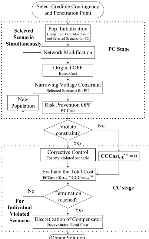
The whole algorithm will be based on genetic algorithm (GA) with the continuous variable are solved using the numerical method based on primal-dual interior point and the discrete variables are solved using the GA procedures. One population in GA will represent one solution. The whole solution is presented in Fig5 consist of two main part called preventive control (PC) and corrective control (CC) parts. Addressing proper scenarios into PC or CC stages will confirm the optimal solutions.
1) Preventive Control Part
After defining scenarios (contingency and VRE penetration point) the algorithm in the upper dashed-box will decided the compensator tap position, generator output limit and selecting scenarios randomly as further explain in [22]. After manipulating the new constraint, the new generation
cost consist of PC cost will be obtained for every population. If there is no violation for all scenarios within a population the total cost is the PCCost. However, for a population having violated scenario after the PC stage will be executed in the CC stage (lower dashed-box).
2) Corrective Control Part
For any violated scenarios within one population, the prepared corrective control will be calculated individually using the algorithm in this box following the corrective control scheme presented by the objective function in eq. (16). Depending in the number of violated scenarios remained in each population, CC stage part will be oftently acces or not which can become the computation burden. 3) Total Cost Evaluation
For evaluating the total cost for a population, since the violated scenarios are not going to really occur the CC cost may be unneccesary to be paid. For this reason, it is belong to the “may be paid” group which should be weighted by the scenario’s occurrence probabilities.
The optimal management between CC and PC stages are determined by the procedures presented in the flowchart. Fig 4 Phylosophy of the proposed method
Network Modification
Violate constraint?
Narrowing Voltage Constraint Selected Scenario for PC
CCCostr-kvio= 0
Evaluate the Total Cost PCCost+ Σ Ar-kvioCCCostr-k
vio
New Population
Termination reached?
Obtain Solution Yes No
Original OPF Basic Cost
Risk Prevention OPF
PCCost
Yes
No
Corrective Control For any violated scenario Select Credible Contingency
and Penetration Point
Pop. Initialization Comp. Tap, Gen. Max Limit and Selected Scenario for PC
Selected Scenario Simultaneously
For Individual
Violated Scenario
PC Stage
Discretization of Compensator
Re-evaluate Total Cost
CC stage
Initially the scenarios for PC stage are selected randomly by the population generation process, then final evaluation is determined by the total cost. For evaluation purpose, the CCCost for any violated scenario should be weighted by the scenarios probability as presented in this equation:
GaNbTGUa = 'ccGUa + ∑ d.[38)\ cccGUa.[38)\ (20)
With:
'cTGUa = (21) cccGUa.[38)\ = Z8)\.[3 (22) E. Simulation Set Up
The simulation are conducted in modified IEEE 57 test system in stressed operating point for voltage stability monitoring purpose, which the VRE penetrate at bus 14, 18 and 56 with the output for the upcoming time-slot are 9, 12 and 7 MW respectively, with controllable capacitor bank at 18 and 34 while the reactor at bus 25 and 46, each with the maximum compensation value 1 Mvar. Those compensators have 10 taps regulations. The total load is 576 MW and the economic load dispatch without considering any uncertainty resulting in the average operating cost at 15463 unit cost. For the base case, line contingency are considered at line 5, 19, 20 and 53, so in total there will be 135 considered scenarios with given occurrence probability.
All of the simulations is conducted using MATLAB, with the MATPOWER [29] for solving the power flow equation and HCOPF solver [22] for solving the OPF using 64-bit PC with 3.00 GHz CPU and 32 GB memory. The voltage stability problem is evaluated using the technique presented in [28]. The traditional solution which solves the problem only by the preventive scheme are used as the comparison.
III.RESULT AND DISCUSSION
The effectiveness of the proposed method is demonstrated using two scenario cases, a base scenario with 135 scenarios and larger scenarios with 810 scenarios. There are three control strategies to be compared for showing the merit of the proposed method. Those control strategies are:
• Trad for the original HCOPF
• Prop1 for the proposed method with discretization
• Prop2 for the proposed method without discretization
The difference between Prop1 and Prop2 is how to generate the compensator tap status. Since the status of the compensator is a discrete variable, the solution should be chosen from the population generation stage (Prop1). However, the computation burden is more substantial. Therefore, the simplification for ignoring the compensator as a discrete variable can be made, which can be included in the digital process for both CC and PC stages. The final value of the discrete variable will be normalized after the final evaluation process.
A. Base Scenario
Base scenario considers 135 scenarios, 27 scenarios at non-contingency and 108 scenarios at contingency. There are 3 methods that should be considered that are Trad, Prop1, and Prop2. The Trad method focus on solving as many scenarios as possible in the PC stage and the remaining violated scenario in CC. Prop1 and Prop2 manage the scenarios to be handled in PC and CC simultaneously. The difference between Prop1 and Prop2 are the consideration of reactor and capacitor as a discrete variable (1) and a continuous variable (2) for the CC.
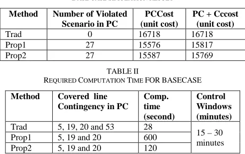
It can be inferred from Table 1 that the Trad method can secure all of the scenarios with the generation cost 16718 unit cost compared to the 15463 for not considering the uncertain scenario. Even if, the system can secure all scenarios the generation cost dramatically increases. The proposed method is choosing the scenarios for PC and CC, consider the occurrence probability and also severity, for that reason the generation cost is still below the Trad, which result in 15576 and 15587 unit cost, respectively. It is proved that the proposed method achieves a more economical operating point. The cost allocation for the base scenario are presented in Fig 6 shows that the proposed method can optimize the total cost by managing the PC and CC stages (Trad algorithm only focus on the PC stage). Since some scenarios are not likely going to happen, it is wise for intentionally managing those into CC stage only even some risk remain (existence of grey zones). From the risk existence point of view, the Trad is better since no grey zones remained even the total cost is very high.
From the computation burden, modifying HCOPF [22] into some subproblems (CCCost algorithm) increase the TABLEI
BASE CASE SIMULATION RESULT
Method Number of Violated Scenario in PC
PCCost (unit cost)
PC + Cccost (unit cost)
Trad 0 16718 16718
Prop1 27 15576 15817
Prop2 27 15587 15769
TABLEII
REQUIRED COMPUTATION TIME FORBASECASE
Method Covered line Contingency in PC
Comp. time (second)
Control Windows (minutes)
Trad 5, 19, 20 and 53 28
15 – 30 minutes
Prop1 5, 19 and 20 600
Prop2 5, 19 and 20 120 Fig 6 Cost allocation for base scenario
14800 15000 15200 15400 15600 15800 16000 16200 16400 16600 16800 17000
Trad Prop1 Prop2
T
o
ta
l
C
o
st
(
U
ni
t
C
o
st
)
computation burden, since the subproblem should be xecuted in each iteration. It described in Table 2 that the computation time is increasing for the proposed method, especially when the subproblem still consists of the discrete variable. However, the computation times are still acceptable for each method since the efficient control window lies between 15-30 minutes.
B. Extended to Larger Scenario
Considering larger scenario by considering line contingencies 2, 3, 5, 7, 8, 12, 14, 15, 19, 20, 23, 24, 25, 27, 30, 35, 38, 39, 47, 53, 59, 60, 61, 63, 64, 65, 71, 78, and 79 in the formulation problem, the problem size will be larger since 810 scenarios should be considered in the problem. The results are shown in Table 3, in which the traditional method solution is not feasible for the Trad. Therefore, the CC is needed. Trad will use the operating point from the CC result and executed the CC individually when the scenarios occur. The risk cost is calculated using the same manner as the penalty cost [22].
On the other hand, the Prop2 solution is feasible for a complete solution solver. Moreover the total cost is more economical than the trad, even if the PCCost is more expensive. From this case, it can be inferred for some heavy loading condition case that, it will be not possible trying to solve all of the scenarios in the PC stage, like the traditional. Risk management of the proposed method once against showing the merit of the proposed method over the Trad. From the cost allocation, it can be inferred that scenarios selection management by the proposed method confirms the more economical total cost. Moreover, the grey zones of Trad is very large, which means the Trad algorithm is not effective for very large scenarios resulting in a higher penalty cost. In this case, the proposed method has better performance in both cost and risk minimization, which is rather different from the base scenario. Considering only the “must be paid” cost (pink and blue zones), Trad has less expensive cost. However, the risk cost is too high. Usually, the power system utility will not operate their system in a high-risk option.
Both algorithms try to eliminate the scenario related to line-20 contingency, which is the most severe from the voltage stability problem [28]. From the computation speed aspect, it can be inferred that the proposed method is consistently longer than Trad as shown in Table IV. However, both of them still acceptable for the practical use. C. Performance in the corrective scheme
Looking closer to larger scenarios, which both of them still result in a violated scenario after PC stage, the system stability and security is evaluated using the tools presented in the previous section. The comparison between Trad and Prop2 described in Fig 8Error! Reference source not found. and Fig 9Error! Reference source not found.. Those figures describe the severity of voltage stability performance for the violated scenarios, in which the voltage stability is dramatically decreased after the contingencies. Normal indicates the non-contingency and VRE as a predicted scenario. N-1 indicates one of the contingency scenario (in this case line-20 contingency), and N-1x indicates the operation point after the CC (load shedding).
N-1x indicates the safe operation point after CC. Both of the control strategies having the potential violated scenarios can secure the operating point after CC. From those figures, it can be inferred that distance to the safe operation (lie between the dash lines) for the proposed method is closer than Trad. It is shown that the required amount of load shedding is smaller than Trad (2.27 MW compare to 3.39 MW). Therefore, the proposed method warrant a more economical operating point.
TABLEIII
LARGER CASE SIMULATION RESULT
Method Number of Violated Scenario in PC
PCCost (unit cost)
PC+CC cost (unit cost)
Trad 18 15487 18481
Prop2 18 15965 17176
TABLEIV
REQUIRED COMPUTATION TIME FOR LARGER CASE
Method Covered line Contingency in PC
Comp time (second)
Trad All except 20 234
Prop2 All except 20 858
Fig 7 Cost allocation for larger scenario
Fig 8 Corrective scheme in the Trad
Fig 9 Corrective scheme in the Prop2 13500
14000 14500 15000 15500 16000 16500 17000 17500 18000 18500 19000
Trad Prop2
T
o
tal
C
o
st
(
U
ni
t
C
o
st
)
One more advantage that the proposed method has is for every numerical method there is always a feasible solution, which the global optimum is confirmed even the considered scenario is very large. The existing methods presented in the previous section did not guarantee the feasible solution for the very large scenario.
IV.CONCLUSIONS
Extending the HCOPF into the proposed method gives us more flexibility which can summarize as follow: Controlling the generation cost is possible for obtaining more economical operating point which showing the proposed method can optimize the management between PC and CC stages. Any larger problem can be feasible since the computation burden in PC stage can be controlled, then shift to the CC stages even if the risk cost will be very high. Even if the computation time is quite increasing, the computation time is still feasible for the control and operation purposes.
NOMENCLATURE Sets
index for generators.
Q, m ithe ndex for buses.
index for buses with reaca tive power compensator.
H index for VRE scenario.
@ index for line contingency scenario.
S number of generators.
W number of buses.
number of injected VRE buses number of VRE scenarios.
number of considered line contingency scenarios. number of total scenarios (VRE and contingency)
Z number of buses which are available to curtail. Variables
generation cost ('ccGUa).
Z8)\.[3 corrective cost (cccGUa).
d. occurrence probability of VRE scenario.
N, n and T are generator cost coeficient.
'(-). generator active power dispatch.
2(-). generator reactive power.
'(-) generator active power without affected by VRE.
'( 0) generator reserve power.
J) generator power reduction coefficient.
4 678 .3 voltage stability index (VSI) of the most severe bus.
'E5R active power demand.
'5 . VRE’s power.
'XY*.3 load curtailment amount for load shedding (LS).
2E5R reactive power demand.
NO+ reactive power compensator tap position.
23+. reactive power of reactive compensator.
2 7L+ reactive power of each tap unit.
'E5. net active power.
2E5.3 net reactive power.
S5*3 line conductance.
W5*3 line susceptance.
V5*.3 voltage angle difference.
5*.3 line apparent power flow. dH−@t G Probability of violated scenario Bounds
* 15* line loading limit.
'()*)+ lower bound of generators’s active power.
'()* 1 upper the bound of generators’s active power.
2()*)+ lower bound of generators’s reactive power.
2()* 1 upper the bound of generators’s reactive power.
45*)+ lower bound of buses’s voltage.
45* 1 upperthe bound of buses’s voltage.
NO+*)+lower bound of reactive power compensator’s taps. NO+* 1 upper bthe ound of reactive power compensator’s taps.
ACKNOWLEDGMENT
This research topic is strategic for supporting the renewable energy integration into the national grid, which the integration level is 23% in 2025 as mention in National Energy Policy.
We would like to thank the ministry of research and education of Indonesian Republic through the competitive research grant with the title “Study Integrasi Pembangkit Energi Baru dan Terbarukan pada Jaringan Listrik Nasional” number 129/UN1/DITLIT/DIT-LIT/LT/2018.
We gratefully acknowledge the funding from USAID through the SHERA program – Centre for Development of Sustainable Region (CDSR).
REFERENCES
[1] L. Platbrood, F. Capitanescu, C. Merckx, H. Crisciu, and L. Wehenkel, “A Generic Approach for Solving Nonlinear-Discrete Security-Constrained Optimal Power Flow Problems in Large-Scale Systems,” IEEE Trans. Power Syst., vol. 29, no. 3, pp. 1194–1203, May 2014.
[2] F. Capitanescu, D. E. M. Glavic, and L. Wehenkel, “Contingency filtering techniques for preventive security-constrained optimal power flow,” IEEE Trans. Power Syst., vol. 22, no. 4, pp. 1690–1697, 2007.
[3] F. Capitanescu and L. Wehenkel, “A new iterative approach to the corrective security-constrained optimal power flow problem,” IEEE Trans. Power Syst., vol. 23, no. 4, pp. 1533–1541, 2008.
[4] L.-A. Dessaint, I. Kamwa, and T. Zabaiou, “Preventive control approach for voltage stability improvement using voltage stability constrained optimal power flow based on static line voltage stability indices,” IET Gener. Transm. Distrib., vol. 8, no. 5, pp. 924–934, May 2014.
[5] L. M. Putranto, R. Hara, H. Kita, and E. Tanaka, “Risk-based voltage stability monitoring and preventive control using wide area monitoring system,” in 2015 IEEE Eindhoven PowerTech, PowerTech 2015, 2015.
[6] T. V. Menezes, L. C. P. da Silva, C. M. Affonso, and V. F. da Costa, “MVAR management on the pre-dispatch problem for improving voltage stability margin,” IEE Proc. - Gener. Transm. Distrib., vol. 151, no. 6, p. 665, 2004.
[7] Su Su and K. Tanaka, “An efficient voltage stability ranking using load shedding for stabilizing unstable contingencies,” in Proceeding of 44th International Universities Power Engineering Conference, 2009.
[9] R. Billinton, R and Karki, “Maintaining supply reliability of small isolated power systems using renewable energy,” IET Gener. Transm. Distrib., vol. 148, no. 6, pp. 530–534, 2001.
[10] California Independent System Operator, “Integration of Renewable Resources,” 2007.
[11] Australian Energy Market Operator, “100 Percent Renewables Study – Modelling Outcomes,” 2013.
[12] Price Water Cooper, “100% renewable electricity A roadmap to 2050 for Europe and North Africa,” 2010.
[13] IEC, “Grid Integration of Large-capacity Renewable Energy sources and use of large-capacity Electrical Energy Storage,” 2012. [14] MIT Energy Initiative, “Managing Large-Scale Penetration of
Intermittent Renewable Energy,” 2011.
[15] Sustainable Energy Quanta Technology, “Grid Impacts and Solutions of Renewables at High Penetration Levels,” 2009.
[16] N. R. Tummuru, M. K. Mishra, and S. Srinivas, “Dynamic Energy Management of Renewable Grid Integrated Hybrid Energy Storage System,” IEEE Trans. Ind. Electron., vol. 62, no. 12, pp. 7728–7737, Dec. 2015.
[17] P. Pinson, “Uncertainties in Renewable Power Generation and Electric Loads,” in Tutorial material at Power System Computation Conference, 2016.
[18] A. Ulbig and G. Andersson, “Analyzing operational flexibility of electric power systems,” Int. J. Electr. Power Energy Syst., vol. 72, pp. 155–164, 2015.
[19] M. P. and L. S. C. Hamon, “Applying stochastic optimal power flow to power systems with large amounts of wind power and detailed stability limits,” in Optimization, Security and Control of the Emerging Power Grid (IREP), 2013 IREP Symposium, 2013, pp. 1– 13.
[20] L. M. Putranto, R. Hara, H. Kita, and E. Tanaka, “Multistage preventive scheme for improving voltage stability and security in an integrated renewable energy system,” IEEJ Trans. Power Energy, vol. 137, no. 1, 2017.
[21] L. M. Putranto, R. Hara, H. Kita, and E. Tanaka, “Multistage Preventive Scheme for Improving Voltage Stability and Security in
an Integrated Renewable Energy System,” IEEJ Trans. Power Energy, vol. 137, no. 1, 2017.
[22] L. M. Putranto, R. Hara, H. Kita, and E. Tanaka, “Hybrid computation approach for SCOPF considering voltage stability and penetration of renewable energy,” in 19th Power Systems Computation Conference, PSCC 2016, 2016.
[23] K. Karoui, H. Crisciu, A. Szekut, and M. Stubbe, “Large-Scale Security Constrained Optimal Power Flow,” in Power System Computation Conference, 2008, pp. 1–7.
[24] J. Mohammadi, G. Hug, and S. Kar, “A Benders Decomposition Approach to Corrective Security Constrained OPF with Power Flow Control Devices,” 2014.
[25] Y. Xu, Z. Y. Dong, R. Zhang, K. P. Wong, and M. Lai, “Solving Preventive-Corrective SCOPF by a Hybrid Computational Strategy,” IEEE Trans. Power Syst., vol. 29, no. 3, pp. 1345–1355, May 2014. [26] S. Li, Y. Li, C. Yijia, T. Yi, L. Jiang, and B. Keune, “Comprehensive
decision-making method considering voltage risk for preventive and corrective control of power system,” IET Gener. Transm. Distrib., vol. 10, no. 7, 2016.
[27] Zwe-Lee Gaing and Rung-Fang Chang, “Security-constrained optimal power flow by a mixed-integer genetic algorithm with arithmetic operators,” in 2006 IEEE Power Engineering Society General Meeting, 2006, p. 8 pp.
[28] Y. Gong, N. Schulz, and A. Guzman, “Synchrophasor-Based Real-Time Voltage Stability Index,” in 2006 IEEE PES Power Systems Conference and Exposition, 2006, pp. 1029–1036.