Published online May 30, 2014 (http://www.sciencepublishinggroup.com/j/acm) doi: 10.11648/j.acm.20140303.11
A numerical algorithm for the resolution of scalar and
matrix algebraic equations using Runge-Kutta method
Tahar Latreche
Doctorate student in Civil Engineering, B.P. 129 Salem Lalmi, 40003 Khenchela, Algeria
Email address:
To cite this article:
Tahar Latreche. A numerical Algorithm for the Resolution of Scalar and Matrix Algebraic Equations Using Runge-Kutta Method. Applied and Computational Mathematics. Vol. 3, No. 3, 2014, pp. 68-74. doi: 10.11648/j.acm.20140303.11
Abstract:
The Runge-Kutta method is an interesting and precise method for the resolution of ordinary differential equations. Fortunately, when supposing the differentiation by any variable that the equation to solve is not variable of, and after iterations, the solution of this equation stretches to the algebraic roots of this equation. This feature of this algorithm, indeed, allows to solve precisely any scalar or matrix equation. The numerical algorithm proposed herein is an iterative procedure of the fourth-order Runge-Kutta method with an adopted precision tolerance of convergence. Also, a method to determine all the roots of the polynomial equations is presented. Some scalar and matrix algebraic equations are resolved using this proposed algorithm, and show how this algorithm featuring with an excellent precision, a good speed and a simplicity for programming to solve equations and deduct the roots.Keywords:
Algebraic Equations, Linear and Non-Linear Algebra, Elementary Equations, Polynomial Equations, Runge-Kutta Method1. Introduction
Indeed, that there’s a lack in mathematics and numerical analysis of theoretical methods or really good precision algorithms or techniques for solving scalar or matrix, as well as real or complex algebraic equations [1-10], especially when these equations being too complex, and when the theoretical mathematics stays be unable to propose a theoretical solution.
The Fourth-Order Runge-Kutta R-K method is a precise and a converged method for the resolution of the Ordinary Differential Equations, and is an effective, efficiency, and the most useful method in the science and engineering practices [1-10]. The special case when we would integrate the Ordinary Differential Equation ODE with any variable which the main equation is not function of, this case indeed, automatically implicate that the proposed ODE will becoming an Algebraic Equation AE, and the seeking solution being the AE root.
Moreover, the roots of the getting AE cannot be precisely occurring by the first resolution of this equation using the R-K method, because that these roots are unknown and; but the started roots of this AE don’t be in general the exact roots needed. If we start our search of roots from a scalar zero or a null matrix or a vector, so we should need a
sufficiently number of iterations of the R-K method, according to the precision sought, for the root we want getting of the proposed AE. Thus, for any so simple or complex elementary functions algebraic equations, it shall only to iterate the fourth order Runge-Kutta method till the convergence will be checked. For the Algebraic Polynomial Equations, an algorithm allows us to deduct all the roots of any degree of these equations is proposed.
In fact, this proposed algorithm is concerning any AEs that have real or complex roots, and when an Algebraic Equation has no real roots, this equation converge iteratively to the close point from zero, or the null vector or matrix, and then start diverging, so we can conclude that we should apply the complex equations technique.
universal problems in science and engineering. Some scalar and matrix AEs are presented and resolved using this algorithm, and the resulting illustrations of the iteration loops allow us to remark that this proposed numerical algorithm is effectively, simple, useful and very precise to solve any scalar or matrix AEs for the science and engineering practices.
2. The Elementary Functions Equations
The elementary functions algebraic equations represent a part of complex mathematical equations. For these algebraic equations, like all the algebraic equations, the iteration procedures of the Fourth-Order-Runge-Kutta method, preferred to starts with scalar zero or null vector or matrix with a so small step of the variable dividing of, and of the tolerance of convergence (the tolerance of the convergence can be controlled, by the way of the convergence of the equation to resolve or, the differences between root iterations). Anyway, the algorithm is very simple, such that it iterates on the Runge-Kutta method until the convergence is checked.
Although, we should indicate that some programming languages, don’t contain the elementary functions of vectors or matrices, and so we have evaluate these kind of functions using Taylor series. We should to indicate herein too, that we shall avoid starting the roots with the absolute scalar zero or null vector or matrix, for some equations contains indefinite functions in these abscissas like the functions or .
The iterative algorithms, for the resolution of a scalar and matrix algebraic equations and , are formulated as follows:
0 0.5 0.5
! 2 2 ⁄6
%
(1)
And,
0 & & 0.5& & 0.5& & & ! & 2& 2& & ⁄6
%
(2)
Where, is the step of the variable divided by, ' is the scalar root and ' the matrix root for the () iteration of the elementary functions equations and ,
respectively. * and &* are the +() scalar and matrix Runge-Kutta method coefficients.
The checking of the convergence is given by the logical expressions:
, -. / and, 0, 2 , -. / Such that -. / is the convergence needed.
As an example, the FORTRAN algorithm for the resolution of the equation 5 3 -.4 56 0 is obtained by the instructions:
K = 0 X = 0. DT = 0.0005
CONV = 0.00000000001 DO
K = K + 1
K1 = DT*(5. - COS(X)*EXP(X))
K2 = DT*(5. - COS(X+0.5*K1)*EXP(X+0.5*K1)) K3 = DT*(5. - COS(X+0.5*K2)*EXP(X+0.5*K2)) K4 = DT*(5. - COS(X+K3)*EXP(X+K3))
X = X + (K1+2.*K2+2.*K3+K4)/6. EQA = 5. - COS(X)*EXP(X) IF(ABS(EQA)<CONV)EXIT ENDDO
WRITE(*,*)K,X,EQA After execution, we get:
& 1687
4.755426629255660
<=> 9.504397269211040E 3 012
3. The Polynomial Equations
The polynomial equations have a special consideration in science and engineering, because of their considerable use and applicability in practice. The values and Eigen-vectors problems or the Optimal Control Matrix Riccati equation are two examples of their applicability. The method proposed herein; present an algorithm to follow for the reason to find all the roots of any polynomial equation, using of course the iteration on the Runge-Kutta method to resolve.
Suppose that we have the arbitrary Polynomial Equation of degree :
AB B CB B CB B D C 0 (3)
Such that C' are the constant coefficients of this equation, and represent the roots of AB 0, and such that the upper index “1” of C' represent the first polynomial equation given AB 0.
3.1. Viète Theorem
The roots of any polynomial equation, like the polynomial given by equation (1), and its coefficients shall be satisfying the following relations:
CB 'E 31 'F' 1, 2, …
Where F' are elementary symmetric functions of
, , … B:
F H '
B
I
F H J
B
K LJ
F H J '
B
K LJL'
M
FB … B
3.2. The Method to Find the Roots
Suppose that we have the polynomial scalar equation of degree given by (3) or the polynomial matrix equation:
AB B NB B NB B D N 0 (4)
such that N' are the matrix constants coefficients, are the matrix or vector roots of the matrix equation (4) and its degree. The upper index N' has the same definition as
C'.
Suppose that, the scalar O or the matrix or vector are given by:
O 40P QCB R, FSTUQNB R (5)
Such that, 40P C' is the scalar sign of C' , and
FSTU N' is the matrix sign of N' , and for a constant
coefficient NV* the outer index + represent the incremental number, though the lower index W represent the number of the constant coefficients in the polynomial equation.
Thus, the first scalar root of AB and AB , iterating on 0 X 1 until convergence, are given by:
0 AB
AB 0.5
AB 0.5
AB
31 BE O 2 2 ⁄6
%
(6)
And,
0 & ABQ R
& ABQ 0.5& R
& ABQ 0.5& R
& ABQ & R
31 BE & 2& 2& & ⁄6
% (7)
Where, * and &* are the same as declared in section 2. is the first scalar root and the first matrix or vector root for the 0() iteration of the polynomials equations AB and AB , respectively.
The checking of the convergence is too, expressed in section 2. Replacing by AB and by AB .
For the remaining scalar or matrix or vector roots, we shall to solve the getting polynomial equations, every time after decomposition and decline the preceding root. For the
1 () roots (1 Y Y 3 1), the polynomial equations
become:
AB ' B ' CB ''E B ' CB ' 'E B ' D C'E 0 (8)
AB ' B ' NB ''E B ' NB ' 'E B ' D N'E 0 (9)
Where,
O 40P Q B ' C
B ' ' B ' CB ' ' B ' D C 'R
CB ''E CB 'E ' '
CB ' 'E CB '' CB ''E '
CB ' 'E CB ' ' CB ' 'E '
M
C 'E C ' C 'E '
%
(10)
'E 0
AB 'E
AB 'E 0.5
AB 'E 0.5
AB 'E
'E 'E 31 'E O 2 2 ⁄ .Z [6 3 1
B 3C B 3 CB B .Z 3 1
%
(11)
The same algorithm would be get, by changing small letters by capital ones, we obtain:
FSTUQ B ' N
B '' B ' NB ' ' B ' D N 'R
NB ''E NB 'E ' '
NB ' 'E NB '' NB ''E '
NB ' 'E NB ' ' NB ' 'E '
M N'E N ' N 'E
'
%
(12)
'E 0
& ABQ 'E R
& ABQ 'E 0.5& R
& ABQ 'E 0.5& R
& ABQ 'E & R 'E 'E 31 'E O & 2& 2& & ⁄ .Z [6 3 1 B 3NB 3 N B B .Z 3 1
%
(13)
The following FORTRAN listing, represent the algorithm to resolve the polynomial equation:
AB \3 32 ]3 33 3 2468 9596 3 2400 3 14400 0
N = 6 L = 6 DT = 0.0001
CONV = 0.00000000002 B(1,N) = -32.
B(1,N-1) = -33. B(1,N-2) = -2468. B(1,N-3) = 9596. B(1,N-4) = -2400. B(1,N-5) = -14400. D = B1(1,N)
DO I = 1, N - 1
K = 0 X = 0.
SIGNE = (-1)**(L+1)
DO
K = K + 1
K1 = X**L DO LL = 1, L
K1 = K1 + B(I,LL)*(X**(LL-1)) ENDDO
K1 = REAL(DT)*K1
K2 = (X+0.5*K1)**L DO LL = 1, L
K2 = K2 + B(I,LL)*((X+0.5*K1)**(LL-1)) ENDDO
K2 = REAL(DT)*K2
K3 = (X+0.5*K2)**L DO LL = 1, L
K3 = K3 + B(I,LL)*((X+0.5*K2)**(LL-1)) ENDDO
K3 = REAL(DT)*K3
K4 = (X+K3)**L DO LL = 1, L
K4 = K4 + B(I,LL)*((X+K3)**(LL-1)) ENDDO
K4 = REAL(DT)*K4
EQA = X**L DO LL = 1, L
EQA = EQA + B(I,LL)*(X**(LL-1)) ENDDO
IF(ABS(EQA)<CONV)EXIT
ENDDO
10 WRITE(*,*)K,X,EQA IF(K==0)EXIT L = L - 1
D = X**L DO LL = 1, L-1
D = D + A(I,LL)*(X**(LL-1))
ENDDO
B(I+1,L) = B(I,L+1) + X DO LL = L-1, 1, -1
B(I+1,LL) = B(I,LL+1) + B(I+1,LL+1)*X ENDDO
IF(I==N-1)THEN X = -B(I+1,L) K = 0
EQA = X + B(I+1,L) GOTO 10
ENDIF ENDDO
The output results of this equation are the following:
& 23, 1.999999999999998, <=> 31.807620719773695< 3 011 & 62, 31.000000000000001, <=> 31.942623839568114< 3 011 & 43, 312.000000000000000, <=> 1.455191522836685< 3 011 & 8233, 3.999999999999392, <=> 1.983835318242200< 3 011 & 8532, 5.000000000000021, <=> 31.999467258428922< 3 011 & 0, 329.999999999979420, <=> 0
%
4. Complex Roots
Indeed, that there are be infinite equations that have no real roots; the complex solutions in this case represent the roots of such equations. As examples of these equations
-.4 ! 2 0, 56 1 0,
1 0 and so on. The proposed algorithm is also available to solve these equations of complex roots. We have then to declare the equation or AB , the roots , the coefficients of the Runge-Kutta method and as complex variables, and the method is available for matrix equations or polynomial equations. The resolution of the equation
56 7 0 in the FORTRAN code can be listing
by the algorithm: K = 0
X = 0.
DT = (0.001,0.001) CONV = 0.00000000001
DO
K = K + 1
K1 = DT*(7. + EXP(X))
K2 = DT*(7. + EXP(X+0.5*K1)) K3 = DT*(7. + EXP(X+0.5*K2)) K4 = DT*(7. + EXP(X+K3))
X = X + (K1+2.*K2+2.*K3+K4)/6.
EQAC = 7. + EXP(X)
IF(ABS(REAL(EQAC))<CONV.AND.ABS(IMAG(EQAC ))<CONV)EXIT
ENDDO
WRITE(6,*)K,X,EQAC The obtained results are:
& 4148
1.945910149053894 03.141592653591149
<=> 9.936940159605001< 3 012 0 3 9.486664654775595< 3 012
5. Numerical Examples
• Example 1
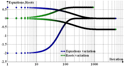
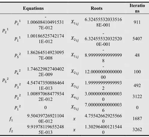
The first example extend and illustrates the variations of the matrix algebraic equation A 3 > 0 and its roots, such that represent the square-roots matrices of the matrix >. The matrix > is a 5 ^ 5 such that all the elements of this matrix J 2. The figure 1, Shows the converged variations of the elements of the matrix polynomial equations A and A and their roots elements versus the iterations numbers. The Table 1, offers the final converged results of A and A and their roots elements and the numbers of iterations needed for the convergence.
• Example 2
In this example we show illustratively and numerically the results of the resolution of the matrix polynomial equation:
A] ] N] N N N N 0
Such that all the composed matrices of this equation are
5 ^ 5 and, the constant matrices elements are given by:
C] J 9, C J 3515, C J 311925, C J 443250, C J 32835000
Figure 2, shows the curves of the variations of the initial polynomial equation A] , and the derived polynomials equations elements, versus the numbers of iterations needed for the convergence; though, Figure 3, illustrates the variations of the roots elements. The Table 1, shows the final converged results.
Figure 2. The variations of the polynomial matrix equation and the equations derived (Example 2)
Figure 3. The variations of the polynomial matrix roots (Example 2)
• Example 3
In this example, we resolve the elementary scalar equation 5 3 56-.4 0. Figure 4 and Table 1, show and illustrate the results.
Figure 4. The variations of the equation and its root vs. iteration (Example 3)
• Example 4
We are occupied in this example to solve the scalar equation -.4 3 0. The variations of and are shown by Figure 5. Although, the final converged results are given by Table 1.
Figure 5. The variations of the equation and its root vs. iteration (Example 4)
Table 1. The converged final results of the Examples 1, 2, 3 and 4
Equations Roots Iteratio
ns
A
A 1.00608410491531
-7E-012 J
6.32455532033516
8E-001 911
A 1.001865257421741E-012 J
-6.32455532032520
0E-001
5407
A]
A] 1.862645149230957E-008 J
-8.99999999999999
8
48
A 1.746229827404022E-009 J
-12.0000000000000
00
100
A 4.547473508864641E-013 J 1.999999999999932 492 A 1.008970684779342E-012 J 3.000000000000030 3122
A 0 ] J 7.00000000000003
6 0
9.50439726921104 0E-012
4.75542662925566
0 1687
9.91978119655248 5E-013
1.30296400121544
6. Results and Discussion
Indeed, that the results (the roots) of the examples taken of the different algebraic equations are much converged to the exact solutions. As it is shown by the different Figures and the Table 1, the convergence of the elementary functions equations or polynomials can be exceeds in general 1 10⁄ _, and their roots precision reach the order of
1 10⁄ . As it is shown by Figure 1, and clear by Table 1, that the convergence of the equation approaches to 1 10⁄ and the sum of its total iteration number approaches to
6500 such that its two roots represent the square-roots of the matrix >, and the second root can be simply deducted without iterations, using the algorithm and the Fortran listing instructions of section 3. The matrix polynomial equation of degree 5 of the example 2, its convergence alternates from 1 10⁄ ` to 1 10⁄ and its total iteration number doesn’t exceed 4000. Although, the elementary functions equations of examples 3 and 4, their convergence precision exceeds 1 10⁄ with a number of iterations less than 3500. According to the step adopted, the number of iterations doesn’t exceed 10000, which can take a fraction of a second for the resolution. Moreover, the experience of this algorithm, can allow us to conclude that, when increases, the number of iterations decreases considerably. Also, when we would get good precision, we would of course decrease the tolerance of convergence, and this operation doesn’t in fact, increase the number of iterations greatly. Although, when the tolerance of convergence decreasing, for the reason to get good precision, we have to take in our account probably that this change leads to decrease the step . As it is presented by Table 1, for the polynomials, the numbers of iterations increase considerably from the first equation (the original equation given) to the last equation deducted.
7. Conclusion
As we have indicated that the Runge-Kutta method is a good and precise method for the resolution of ordinary differential equations, and the remark that for constant equations coefficients, the iterative procedure of this method leads to these algebraic equations roots. Although, in the absent of precise algorithms to resolve every real or complex elementary functions or polynomial algebraic equations, the algorithm presented can resolve any algebraic equation with good precision that can regulated as we need such is demonstrated by the arbitrary examples presented (for all the examples presented, the tolerance of convergence at least , 1 10⁄ `). The presented algorithm and the method presented in section 3, allow us to determine all the roots of any matrix or scalar polynomial equation like the scalar polynomials of the Eigen-values and the matrix equations of the Eigen-vectors. The algorithm presented too, is very simple for programming as presented in sections 2, 3 and 4 and some instructions lines can resolve any simple or complex equation. Moreover,
with a personnel computer, any complex equation can be resolved with good precision and as possible, with a small number of iterations. As shown by the Figures presented, that the algorithm automatically refines its roots contributions considerably as possible only and, according to that the exact equation solution is considerably close, and according to the step and the convergence number adopted, the feature that make it very precise and economic algorithm as well in the time of solving and in the iterations numbers. Probably that the algorithm proposed as extended, needs some experience about the step and the tolerance of the convergence; but presents indeed, a new accurate numerical technique for solving any scalar or matrix algebraic equation with good precision and good execution speed, and the method proposed in section 3, for deducting all the remaining roots of polynomials, when the preceding are computed, is in fact a new idea and a new proposal for solving polynomial equations.
As a future development using this algorithm, we will start solving the problem of proper-frequencies (the Eigen-values) and the mode-shapes (the Eigen-vectors) for the semi-explicit solving of the dynamic equilibrium equation of structures subjected to dynamic arbitrary loading. The algorithm too, can be used to solve the two degree Riccati matrix algebraic equation for the optimal control of dynamic systems.
References
[1] Bird, J., (2010). Higher Engineering Mathematics. Sixth Edition, Elsevier, Ltd.
[2] Ciarlet, P. G., and Lions, J. L., (2000). Handbook of Numerical Analysis. Vol. 7. First Edition, Elsevier Science. [3] Kiusalaas, J., (2005). Numerical Methods in Engineering
with Python. First Edition, Cambridge University Press. [4] Polyanin, A. D. and Manzhrov, A. V., (2007). Handbook of
Mathematics for Engineers and Scientists. First Edition, Taylor and Francis Group, LLC.
[5] Press, W. H. et al., (2007). Numerical Recipes. Third Edition, Cambridge University Press.
[6] Press, W. H. et al., (1997). Numerical Recipes in Fortran 77. Second Edition, Cambridge University Press.
[7] Press, W. H. et al., (1997). Numerical Recipes in Fortran 90. Second Edition, Cambridge University Press.
[8] Riley, K. F. et al., (2006). Mathematical Methods for Physics and Engineering. Third Edition, Cambridge University Press.
[9] Soyeur, A. et al., (2011). Cours de Mathématiques. http://www.les-mathematiques.net