Vol.6 (2016) No. 5
ISSN: 2088-5334
A Survey on Adaptation Strategies for Mutation and Crossover Rates
of Differential Evolution Algorithm
Dhanya M Dhanalakshmy
#1, Pranav P
#2, Jeyakumar G
#3#
Department of Computer Science and Engineering, Amrita School of Engineering, Coimbatore, Amrita Vishwa Vidyapeetham, Amrita University, India
E-mail: [email protected]; [email protected]; [email protected]
Abstract— Differential Evolution (DE), the well-known optimization algorithm, is a tool under the roof of Evolutionary Algorithms (EAs) for solving non-linear and non-differential optimization problems. DE has many qualities in its hand, which are attributing to its popularity. DE also known for its simplicity in solving the given problem with few control parameters: the population size (NP), the mutation rate (F) and the crossover rate (Cr). To avoid the difficulty involved in setting of suitable values for NP, F and Cr many
parameter adaptation strategies are proposed in the literature. This paper is to present the working principle of the parameter adaptation strategies of F and Cr. The adaptation strategies are categorized based on the logic used by the authors, and clear insights
about all the categories are presented.
Keywords— Differential Evolution; Parameter Adaptation; Mutation Rate; Crossover Rate.
I. INTRODUCTION
Differential Evolution (DE) (proposed by Storn and Price [1],[2], a population based stochastic search method, is a very powerful algorithm in the repository of Evolutionary Algorithms (EAs). The performance efficacy of DE, comparing with other EAs, for solving real time and benchmarking problems which are non-linear, complex and high dimensional over continuous domain has been well proved in its literature [3]. The algorithmic structure of DE is similar to other EAs. However, unlike other EAs, DE uses very few control parameters: the population size (NP), the mutation rate (F) and the crossover rate (Cr). The efficiency
and accuracy of DE algorithm is more sensitive to the values chosen for these few parameters.
The successful convergence of DE to the global optimum solution, in its evolutionary search for solving the given problem, is largely depend on suitable selection of values for these control parameters. Finding the suitable values for these control parameters, before starting the search, is a difficult task as it will differ from problem to problem. A poor choice of these values will result in the poor accuracy of the algorithm which is not acceptable. There is no single perfect method or standard available for selecting values for these control parameters. Hence, the process of tuning these control parameters along with the search became an attractive area of research for the researchers’ community working in DE. This results numerous adaptation strategies
proposed for NP, F and Cr in DE literature. Subsequently,
this has become a challenge to the practitioners, researchers and users of DE to choose right adaptation strategies for each of the control parameter to solve the problem at their hand. Resolving this challenge is taken as the aim of this paper.
The objective of this paper is to provide the readers with brief insight about various adaptation strategies proposed by researchers for adapting F and Cr. It is obvious that the
number of researchers working in DE, particularly in the parameter adaptation of DE, is increasing day after the other. This paper is intended to provide them with summary of various adaptation strategies exist in DE literature for tuning
F and Cr.
II. DIFFERENTIAL EVOLUTION ALGORITHM
For a search method to be efficient and reliable, it has to cover the entire search space. Differential Evolution starts its search of global solution for the given optimization problem, with randomly selected NPD-dimensional population vectors (individuals/candidates). The initial population is chosen in such a way that the individuals are initialized randomly in order to cover the entire search space. The population vector is represented as Xi,G= {x1i,G, x2i,G . . . . xDi,G}, i ranges from 1
The three evolutionary processes involved in DE are mutation, crossover and selection. Among these the mutation and crossover are called variation operators, which brings changes in the population by altering the values of the components of the individuals in the population. The changes made by these operators create new candidates in the population, thus increasing the diversity of the population. Hence they attributed to exploration phase of the search. On the other hand, the selection process selects the best candidate from a set of candidates. Thus it is for the exploitation phase of the search.
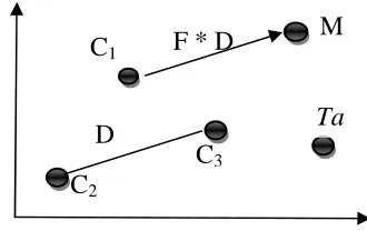
At first the mutation process takes place. From the initial population the mutation process generates a mutated population. This process is termed as Differential Mutation in DE. The mutation process chooses three random candidates (say C1, C2 and C3) from the population, and
generates a mutant vector (MV) as
(1)
where F- mutation rate or scaling factor. In Equ (1), the scaled difference of C2 and C3 is added to C1 (also known as
base vector). There exist many ways to choose the base vector and the other pair of vectors for mutation. Based on that, there are many mutation strategies available for DE. The critical parameter in the mutation process is the scaling factor F. One mutant vector is generated for each vector population (also known as target vector (TaV)) in the current, which results mutated population with NP mutant vectors.
Secondly, the crossover process generates the trial vector (TrV) population. This process recombines each of the TaV in the current generation with its corresponding MV to produce the TrV. The values from the parameters of TaV and MV are used to generate a TrV. The crossover process results one TrV for each TaV. The crossover process determines how much information the trial vector (child) inherits from its parents (target and mutant vectors).This is determined by the control parameter called the crossover rate (Cr). The
most common two crossover strategies of DE are binomial crossover and exponential crossover. The equation for binomial crossover is given in equation (2). The crossover process also repeated for all the pair of target and the corresponding mutant vector, which results a population of NP trial vectors.
TrVi= (2)
Next, a selection process is carried out between each target vector in the current population and their corresponding trial vectors. DE uses one-to-one tournament selection based on the fitness values of the candidates (vectors). The better candidate out of the two will have the privilege to move to the next generation.
Each generation of DE’s search process include these three evolutionary processes (Mutation, Crossover and Selection). The whole process is repeated for G(maximum number of generations) number of generations, which is considered as one run in DE experiment. The best solution
obtained at the end of the run is the solution obtained by DE for the given problem, at that particular run. Since all the stages of evolutionary process in DE (in fact any EA) involves randomness, the average performance of DE algorithm in its many runs is used for reporting its performance.
III.CONTROL PARAMETERS OF DE
Understanding the influence of the parameters of DE (mutation rate (F), crossover rate (Cr) and population size
(NP)) is essential to know the adaptation strategies available for them. This section presents the role of F, Cr and NP.
The mutation process is to alter the values of the components of each of the candidate in the population. The mutation of DE is called as differential mutation, since it uses weighted differences of candidates to perform mutation for the current candidate. One among the unique feature of DE is its differential mutation. The mutation process can be understood from the Figure 1.
Fig. 1.The Differential Mutation of DE.
The Mutation rate (F) (also known as scaling factor, amplification factor, mutation step size or mutation constant) is to scale the distance between the pair of vectors C2 and C3.
This scaled difference is added to the base vector C1. Thus,
the mutation rate is used to control the amplification of the difference vector. Hence, a small value of F will lead to premature convergence whereas a larger value will result in a slower convergence. It controls the range of space where the mutant vectors are generated. Thus, it plays an important role in changing diversity in the population.
In classical DE algorithm the value for F is taken as any real value in the range of 0 to 1. Keeping the value of F as constant will deteriorate the diversity of the population during the search, because all the vectors will be created by same difference vector components. So in order to avoid this, many classical DE implementations follow a different strategy where F will be considered as a random number within the range of [0.2, 0.8]. This ensures that the diversity loss during the search is avoided.
In natural evolution, the crossover process is to create children by inheriting genetic properties from parents. It holds good for DE search also. In this process of genetic inheritance, to get diversified candidate from the parent, the parameter crossover rate (Cr) is used. As similar to F, Cr also
a real valued parameter in the range of 0 to1. It is used to identify the parameters to be inherited from the parents. Crossover rate (Cr) controls the number of elements that the
trial vector will inherit from mutant vector and target vector. Thus it defines how different the child vector is from the
C
2C
3C
1M
D
F * D
parent vectors. In other words, it ensures diversity in the newly created population. Finding the right value of this control parameter is a difficult task as a slight change in the Cr value will affect the efficiency of the algorithm. When Cr
value is approximately equals to 0, DE makes small explorative moves with higher probability of making improvement. When Cr ≈ 0.9, DE makes large explorative moves which helps to perform a more fine-grained search in the solution space and yield large improvements in solution quality.
The third control parameter NP also has significant impact on performance of DE. If NP is small, the search may end in premature convergence, and if it is large the search will take long time to converge. Hence a moderate value for NP, to avoid the premature convergence and stagnation, is acceptable for successful DE search.
There are many methods proposed for adapting F and Cr,
many of them were found to be performing better when compared with classical DE. However, less works are reported in the literature for adapting NP. Hence this paper considers, hereafter, to discuss the existing adaptation strategies for F and Cr.
IV.ADAPTATION STRATEGIES FOR F AND CR
To plan for a suitable adaptation strategy of the control parameters, it is necessary to understand the influence of each of the parameters in the performance of the algorithm.
There are many works reported in literature to discuss the influences of the control parameters. It was in the year 2001, Zaharie [4] was one among the few who started analyzing the possible effect of these control parameter values on DE and their critical values. The approach was both a theoretical and empirical study on how the control parameter values are related with population variance of DE. An equation to measure the critical values of control parameters was derived. The equation derived by Zaharie was 2F2p-2p/m +
p2/m+1=0, where F is the scaling factor, m is the population
size, and p is the crossover rate. The value (F and P) that satisfies this equation was considered critical values. Tremendous efforts have been put by the researcher to analyze the role of each of the DE control parameters. Presenting about them is not in the scope of this paper.
Since the impact of the control parameters MutationRate (F) and CrossoverRate (Cr) on the performance of the
algorithm is very high, many control parameter adaptation techniques has been put forwarded over the years. All of them have been proved as effective and improving the performance of Differential Evolution algorithm in both converge speed and solution accuracy, compared to the classical DE.
The objective of this chapter is to present a brief insight about various adaptation strategies exist in literature. To increase the readability of the paper, the existing adaptation strategies of F and Cr are categorized in to four groups with
respect to the algorithmic methodology followed by the authors. The details of the categories [57] are
• Category 1: Classical Approach
The strategies in this category use mathematical equations to update the values of the control parameters. This updation is done for every generation or at required time.
• Category 2: Encoding of control parameters
Another way of adapting control parameter is to encode the control parameters along with the parametric values of the candidates of the population. Hence, the control parameters also evolve as similar to other parameters. The adaptation strategies following this methodology are grouped under this category.
• Category 3: Deriving from History or Pool
The strategies which use previous information about the performance of the algorithm in the evolutionary search are grouped under this category. The algorithms which maintain pool of values for the control parameters also grouped in this category.
• Category 4: With added logic
The strategies which use some additional technique or algorithm to adapt the parameters are discussed under this category.
A. Classical Approaches
With the understanding of role of F and Cr in the mutation
and crossover processes, the works considered in this category uses mathematical equations derived by the authors to update the values of F and Cr.
In SaDE [5], proposed by A.K Qin and P.N.Suganthan, an adaptive logic for mutation strategy is presented. The mutation strategy is decided based on the success rate calculated for them in the learning period. The F and Cr
values also calculated differently for each of the mutation strategy. For every individual i in the population the F and Cr values for the chosen mutation strategy k is calculated as
follows
(3)
(4)
where is calculated from a success rule as the mean of Cr. This is followed by many researchers for different
applications of DE [6].
The JADE [7][8][9] proposed by Jingqiao Zhang and Arthur C. Sanderson in the year 2007, introduced a new mutation strategy based on the information obtained about the search progress direction. The values of F and Cr are
generated newly for each generation with Cauchy and normal distribution. With the initial values of 0.5, the new values at generations are computed as follows.
(5) (6)
where c , is a constant.
SF and Scr represent the mean of successful values for
crossover rate and scaling factor, respectively. Many other modified DE were introduced which borrowed this concept [10]. In the year 2008, Wu Zhi-Feng proposed a new version of DE called AdaptDE [11]. The fitness values of the trial vector and the target vector are used to find the values for F and Cr. Also, the control parameter values for the G+1th
generation. The fitness values of the trial vector (ftrv) and target vector (ftav) are compared.
/* F and Cr for ith candidate at G+1th generation*/
If ((ftrv<ftav) and (τ1 <randa) and (τ2<randb))
(7)
(8) Endif
If ((ftrv>ftav) and (τ1 >randa) and (τ2>randb)
(9)
(10)
End if
where randa, randb, randc and randd are random numbers
within the range [0.1] and τ1 and τ2 are probabilities for adjusting F and Cr. The authors preferred a value of 0.1 for
both.
In 2009, RadhaThangaraj et al. introduced ACDE [12]. In ACDE, the whole adaptation process is based on few simple rules. Scaling factor for an individual i is defined as
(11)
And Crossover rate is found using the rule,
(12)
where, and refer to random numbers that are Gaussian distributed which has mean and standard deviation of 0 and 1, respectively. The and are random numbers within the range [0,1]. The and represent the probabilities for adjusting Cr and F,
respectively.
The IADE [13] algorithm, introduced by Wenjing Jin et al. in 2010 followed the following adaptation strategy:
• Initially, the values of F and Cr will be fixed as 0.6
and 0.1, respectively.
• It is changed adaptively over the generations.
The mean fitness value of a generation is calculated. To find the F and Cr values for G+1th generation, the mean
fitness value of previous generation (Gth) is compared with the mean fitness value of G+1th generation, and
If Meanfitness(G) >Meanfitness(G+1) then
(13)
(14) Else
) (15) (16)
NasimulNoman, in [14], introduced an approach to use the fitness value of the child and the average fitness value of the population to update the control parameters values. It is done as follows, If fitness values of child is less than average
fitness value then the control parameter values F and Cr at
Gth is taken for their (G+1)th generation. Otherwise,
F
i,G+1= uniform
_rand(0.1,1.0)
(17)
Cr i,(G+1) = uniform_rand(0.0, 1.0) (18)
In 2012, PengGuo et al. proposed SelfDE-F [15]. In SelfDE-F, a secondary population is created with the individuals that were discarded during the selection process of the DE algorithm. The adaptive method for finding control parameter values for each generation was framed as follows
(19)
(20)
where
Fbest,G = Scaling factor of the candidate with best fitness
value. CR_maxG and CR_minG are the maximum and
minimum crossover rate of generation G. The τ1 ,τ2 are two fixed values (Similar to jDE) and rand1, rand2 and rand3 are
uniform random numbers in the range (0,1).
In the same year, Ali W. Mohammed et al. proposed ADE [16]. This paper introduces an alternative differential evolution (ADE) algorithm. In ADE a new mutation scheme is proposed and control parameters are adapted using a defined equation for both F and Cr. Two values of F are
defined, one for the local mutation scheme and the other one for global mutation scheme. Keeping in mind the fact that Cr
must start with a small value and must extend to a larger value as the generations increases, the authors framed an equation to Cr as follows,
(21)
where G is the current generation and GEN is the maximum number of generations.
The authors also mentioned the optimum values for Crmin,
Crmax and K as 0.1, 0.8, and 0.4 respectively.
Ali W. Mohammed et al. also proposed EDE (Effective Differential Evolution) [17]. A simple method for choosing the values for the control parameters is used. The values for Cr and F are chosen empirically from the range of [0.5, 0.9]
a normal distribution N(Crm,0.1). The value for Crm (mean) is
kept as 0.5 and the standard deviation is 0.1.
SAMDE [19] was also introduced in the year 2013 by Xu Wang et al. The SAMDE is similar to JADE. Scaling factor is found using Cauchy’s Distribution with mean µF,
(22)
µF is initialized to 0.5 and then it is changed as,
, (23)
where meanL(SF) is the Lehmer mean
Crossover rate is found from a normal distribution of mean µCR and standard deviation 0.1.
(24) (25) where meanA (SCR) is the arithmetic mean.
Rammohan Mallipeddi and Minho Lee in the same year proposed ESMDE [20], an evolving surrogate (substitute) model-based DE. In ESMDE, based on the current population a surrogate model is created and this is used for selecting appropriate parameter setting so as to creating better off springs during further stages of evolution. Similar to other approaches, the mutation strategies are selected according the concept of pooled values. Here F (scaling factor) is selected randomly within the range of [0.5, 1.0] which ensures that there will be adequate exploration alongside with exploitation. Similarly, Cr value is also
generated randomly from a range of [0,1].
Quizhen Lin et al. proposed an adaptive algorithm [21], in which Cr is found using a framed equation which ensures
that the Cr value will be very large (approximately equal to
0.9) initially and as the generations increases the value decreases and will be stagnant in the range of 0.1 to 0.2. This ensures that the explorative steps taken are very large during the initial phase of the algorithm to favour the global search. As the generations goes the explorative steps will be reduced and the search will be done near local. This ensured good performance of the algorithm. The ScalingFactor is found using a Cauchy's Distributions within the range of (0.5, 0.1). The value for F is selected from a set of successful values collected for F.
Miguel Leon et.al proposed a greedy adaptation of control parameters of DE [22]. Here a greedy search will be performed in learning periods that are successive so as to favour continuous and dynamic adjustments of the control parameters F and Cr. The whole procedure is as follows,
initially the F value is set to 0.5 and two neighbours are defined in such a way that a difference is added and subtracted to the initial F, i.e., . The initial Crossover rate is set to a Cauchy’s Distribution with its centre at 0.5 ( and scale of 0.2. Two neighbours of Cr are and . During the predetermined
learning period, every candidate and it’s neighbouring candidate will have a probability of 1/3 in order to get sufficient number of usages. At the end of the learning period, the best will replace the worst.
Qinqin Fan and Xuefeng Yan proposed another adaptation method [23] to their self-adaptive DE strategy (named as SDE). This is an algorithm with zoning evolution of control parameters and adaptive mutation strategies, called as
ZEPDE. They have defined their own methods to identify the best possible mutation strategies for the DE algorithm. The parameter adaptation is done as follows. The total region of F and Cr are divided into similar sized four areas.
Then at each region the count of control parameter combinations are noted. If the offspring in each zone has a better fitness function value, then it is taken into account that the control parameter combination which gave the best fitness value is the elite one or can be called as Elite Control Parameter Combination (EPC). Assume at the hth, the weighted value of each EPC is computed as follows,
(26)
where
Now the weighted average of control parameters in the hth region is calculated as
(27)
and
(28)
Once the weighted average is calculated the control parameters for the hth generation is calculated using a cauchy’s distribution with mean and and standard deviation (0.55-0.3 *(1-G/Gmax)).
Xiaowei Zhang and Sanyang Liu proposed APFDE [24] in 2011, drawing inspiration from the theory of electro magnetism. They calculated the charge Qi for candidate Xi based on its objective function value and the objective function value of the best candidate in the current generation using the equation given below
(29)
Later, the equation was modified as shown below:-
(30)
where D is the problem dimension and NP is the population size. The Mutant Vector generation in normal DE can be written as follows
(31)
Using the above derivations, F is replaced by Q12 and Q13
respectively. Taguchichi method along with 2-level orthogonal Array is used to set the value of Cr.
generation. The Scale Factor for ith candidate Fi is randomly
picked from a Cauchy distribution with location Parameter Fm and scale parameter 0.1. The list of all F values that
generated better trial vectors are stored in a set Fsuccess. Fm is
updated using the following equation
(32)
Where . Cr is selected
randomly from a Gaussian distribution with mean Crm and
Standard deviation 0.1. The Crm value is updated in each
generation in a similar way as that of F according to the equation given below
(33)
where, . Crsuccess is the set of
all successful Cr values.
Yet another scheme for adapting F and Cr was proposed
in [26], in which the candidates are put into two sorted lists - the first one in descending order based on objective functions and the second one in ascending order based on each candidate’s distance from the best candidate. Then the sum of absolute differences between these two ranks for each candidate is calculated, which is called as Indicator of Optimization State (IOS). Also IOSmin is set to 0 and IOSmax
is calculated using the following equation
(34)
Then IOS is normalized and this normalized value is used to decide whether to explore or exploit. If exploration is to be done, Fg-1 is increased by 1/10th of ΔF and CRg-1 is
decreased by 1/10thΔCR respectively; otherwise Fg-1 is
decreased by 1/10th of ΔF and CRg-1 is increased by 1/10th
ΔCR respectively. ΔF and ΔCR are computed based on IOS,
IOSmax and IOSmin based on the equation
(35)
The mathematical equations used in the studies reported in this section are derived / defined by the authors, based on their understanding about the control parameters and their influences in DE algorithm. It is worth noting that such equations also adds few new terms to it, which are again to be studied further to set proper value for them. This indirectly increases the complexity of parameter adaptations. To avoid this there exist many parameter adaptation strategies for DE control parameters in literature. They allow the values of control parameters also to evolve, as similar to parameters of the candidates, to be better for next generation. Those adaptation strategies encode the control parameters in the parametric representation of the candidates in the population. The next section discusses the strategies with such encoding scheme.
B. Control Parameter Encoding
To avoid inclusion of additional parameters in adapting the required parameters, the idea of encoding the control parameters with the individual candidates in the population arose. This encoding let the control parameters also to evolve along with other parts of the candidates. At the required stages the F and Cr values are selected suitably
from the evolved values of them. Hence, these strategies include efficient selection mechanism to consider the evolved values of F and Cr available at the parent candidates
of mutation and crossover. The works similar to this strategy are discussed in this chapter.
Mahamed G. H. Omran et al. introduced a self-adaptiveDE [27] in 2005. This algorithm uses the differential mutation mechanism to find the new values of F and Cr. Each individual i in the population is encoded with
Fi and Cri, and these values are calculated as follows
(36)
where i1, i2 and i3 are random and distinct candidates chosen
with a uniform distribution U(1,…,NP)
Another self adaptive DE named SADE_ALM (Self Adaptive Differential Evolution with Augmented Lagrange Multiplier) [28][29] was proposed by C. Thitithamrongchai and B. Eua-Arporn in 2006. In the SADE_ALM the F and Cr
are encoded in the first two positions of the candidates. The
F and Cr values are initialized as follows
(37) (38)
Then the F and Cr values are undergoing the mutation and
crossover operations. The mutation process is done as follows:
(39)
(40)
where are non-equal indices between 1 and NP. The crossover process is done as follows:
(41)
(42)
Finally, at required points, the F and Cr values are chosen
improvements of at least half the population. For all the individuals, whose value is greater than this threshold, values are retained and for others new values are randomly generated
In the year 2007, J.Brest et al. put forwarded the jDE algorithm [27][32][33][34][35]. In jDE also, the control parameters F and Cr are encoded with the population along with its genes. These values are adapted during every generation according to two other fixed values 'τ1' and 'τ2'. The value of F in the (G+1)th generation will be same as the value in Gth generation if a randomly created number within the range (0,1) is greater than τ1, else F value is found as
(43)
Suffix 'l' and 'u' stands for lower and upper values of F. Similarly, for Cr if ‘τ2’ is less than randomly generated value then the previous generation value is retained, else
(44)
An enhanced version jDE, named jDE-2 [36], was introduced later with an added concept for keeping the bound-constraints problem feasible. But the parameter control part was kept same as that of jDE.
Brest also introduced a different variant of the above called jDEdynNP-F [37] in 2008, where along with control parameter adaptation, population size reduction mechanism is also implemented. The F and Cr adaptation of the
proposed algorithm remain the same as that of its previous version. Similar adaptation mechanism for F and Cr is
followed by Zhong-bo Hu et al. [38].
Also in the same year Chukiat Worasucheep, proposed wDE [39]. In wDE, a separate strategy adaptation and parameter adaptation is introduced. In parameter adaptation, each individual ‘i’ is extended with corresponding Cri and Fi
which are uniformly initialised within the range [0,1] and [0,2], respectively, at the beginning. A fixed number of generation period (learning period) is considered and adaptation of these control parameters happen after these fixed number of generations. Also two variable nsi and nfi are introduced which indicates the number of success and failure for a particular individual i for entering into the next generation with respect to the learning period. The probability of pass (PPi) for a particular individual i and the average of pass probabilities (PPavg) are calculated. Now, for all those individuals, whose probability of pass is below the probability pass average, the control parameters are updated as follows
(45) (46)
AlesZamuda and BorkoBoskovic in 2007 came up witDEwSAcc [40], Differential Evolution With Self-adaptation and Cooperative Co-evolution. In DEwSAcc also, as similar to other works in this category, all the individuals in the population are extended to include their own control parameters, Fi and Cri. The control parameter value of the
next generation (G+1) depends on the values of these
control parameters of the current generation (G). F and Cr
are updated as follows
(47)
(48)
where, τ represents the learning period which is 1/√D.
In 2008, Omar S. Soliman and Lam T. Bui came up with a self-adaptive strategy to use Cauchy distribution [41]. The control parameters for each individual are encoded along with them. For an individual i, scaling factor is found by
(49)
where, and and are the lower
and upper limit of possible values for scaling factor. Crossover rate is found as follows:
(50)
, k = 0, 1,2,3,4 are uniform random numbers. The probability to adapt F and Cr are denoted by and .
Grant Dick [42] in 2010 defined SaNSDE (self-adaptive neighbourhood search differential evolution) which uses the neighbourhood search which is one of the core concepts of Evolutionary Computing. Control Parameters are added to each individual. It works as follows, the first step is to initialise the CRm value to 0.5 .Then similar to above it is
found during each generation using a normal distribution with mean value CRm and standard deviation 0.1 for each of
the individual. F value is found as follows,
(51)
where is a uniform random number in range [0,1).
The SaFDE [43] proposed by Teng NgaSing et al. encodes scale factor inside each candidate. Initial population has F randomly initialized for each candidate. During trial vector generation, if the random number generated is less than cross over probability, trial vector’s scale factor is also updated in the same way as the other genes using the differential mutation as given below
Here
α
DE is a randomly chosen value between 0 and 1. Ifthe calculated value of F goes beyond the limits [0,1], then it is randomly re-initialized. Authors have self adapted only F and Cr and they are selected randomly from [0.1, 1.0].
each individual. Fi and Cri are updated in each generation
based on two thresholds T1 and T2 as follows:
(53)
(54)
where
r
1, r
2, r
F, and r
Ct are random numbers. Fl is set to0.1 and Fu is set to 0.9. T1 and T2 were set to 0.1.
The above discussed adaptation strategies of F and Cr are
proven to be working better than classical adaptation strategies. They add only little complexity to the algorithm, because it does the changes only in the parametric representation.
C. Deriving from History or Pool
It is also interesting that the future values for the control parameters of any algorithm is decided based on the performance of the algorithm with the past values of the control parameters. There are number of research works reported in DE literature too, in this direction. As well as, all the possible values for each of the control parameters are pooled and the algorithm is allowed to choose the required values based on the present performance of the algorithm. All such works are considered for discussion in this section.
This section is to discuss the adaptation strategies deriving values for the control parameter from the performance history of the algorithm or from corresponding pool of values.
The adaptive DE proposed by Hui-rongetal [45], used previous learning experiences to choose the values for the control parameters. The values of F and Cr are found at each
generation. A random number (rn) with uniform distribution
is generated and
If rn< 0.2
(42)
(55) Else
(44)
(56)
End if
In SHADE proposed by Ryoji Tanabe and Alex Fukunaga [46], the history information about the successful parameter values are maintained to guide DE search. It has a memory to store H values of F and Cr. Then the values for Fi and Cri
are selected form the range [1,H] with a random index ri. Another success history based model known as DEsPA was proposed by Noor Awad et al, in 2015 [47]. Along with
F and Cr the NP value also adapted in DEsPA. Every
individual i in the population is assigned with its own greediness factor pi. A 2-D memory structure stored with the
mean values of F ( and Cr is used for control parameter adaptation. The size of memory (M) is set as half of NP. A random index ri is chosen and is used for
find F and Cr.
(57)
(58)
The EPSDE proposed by R Mallipeddi et al used the concept of pooled values [48]. It consists of a pool of mutation strategies and pools for corresponding parameters for those strategies. The F and Cr values are taken from a
pool which has values within the range [0.1, 0.9] and [0.4, 0.9], respectively. Every step changes the values by 0.1. In EPSDE, each individual in the population is associated with a random mutation strategy taken from the pool. Along with the matched mutation strategy, the corresponding F and Cr
values are also chosen. These values and strategies will survive until the target vector performs poorer when compared with the trial vector. Once this condition is failed, a new mutation strategy will be associated with the target vector. These strategies could be selected from the pool or from the successful combination stored before.
The CoDE [49] algorithm was also introduced in 2011 by Y Wang et al. The parameter values are predefined here. Based on the carefully selected three mutation strategies, the parameter values will be changed. During each generation a set of three trial vectors are generated. On comparison with the target vector, the best of the four (3 trial and 1 target) will go to the next generation. Three combinations are made for F and Cr based on the mutation strategies. It will follow
either of the three defined as [F=1.0, Cr=0.1], [F=1.0, Cr
=0.9] and [F = 0.8, Cr = 0.2].
Wenyin Gong et al. presented a variant of JADE, called
Rcr-JADE in [50], that repairs Cr based on Success history of
Cr values. Cri and Fi are selected from Normal Distribution
and Cauchy Distribution respectively for ith candidate. Then CRi is repaired as per the equation
given below
(59)
where m is the number of genes that were copied from mutant vector and D is the problem dimension. If trial vector Ui is better than target vector Xi, then Cri and Fi are added to
lists of successful Crossover and Mutation Parameters (SCr
and SF). Then is updated as the arithmetic mean of all the
Cr values in SCr. Similarly is updated as the Lehmer mean
of all the F values in SF.
Comparing to other three categories, this category covers very less works in the literature. This is because of the complexity involved in remembering required information from sufficient past time and choosing the values to be achieved in the pool.
D. Parameter Adaptation with Added Logic
Another commonly used strategy for DE control parameter adaptation is to insert an additional component (or algorithm or logic) to the structure of DE. This added component will monitor DE's performance in solving the given problem and suitably adapt the required parameters. The researchers have used some other existing algorithm as the component or have designed their own algorithm. The former one is termed in other words as hybridization of DE with other algorithms.
fuzzy logic controller was used to find the values for F and Cr for the candidate i (Fi and Cri). The FLC-MODE (Fuzzy
Logic Controlled Multi-objective Differential Evolution) [52] was introduced by FengXue et al in the year 2005, as similar to FADE.
An Iterative Function System Based Adaptive DE was proposed by Ya-Liang Li, et. al. [53]. In this algorithm the control parameters are adapted using an iterative function system. The Fi,G and CRi,G values are adapted using the
following equations
(60)
(61)
Here, and are uniformly generated within the range . The parameter is set to 0.5 and is set to 1.
Patricia Ochoa et.al proposed FDE (Fuzzy Differential Evolution), which uses concept of fuzzy system for parameter adaptation [54]. The fuzzy system added to DE will give the best possible values for the control parameters. The fuzzy system has 3 membership functions (FN1, FN2
and FN3) to mean the low, medium and high values of the
parameters. It also used 3 fuzzy rules to update the values of the control parameters.
In 2009, M.G. Epitropakis et al. introduced an evolutionary approach towards self-adapting DE, known as ESADE [55]. In ESADE, a unique strategy was followed in finding the values of the control parameters. It uses two DE algorithms, one is to find the mutation rate (F), and the other for optimizing the given objective function. In the first DE algorithm to find F value, a one-dimensional population is initialized as follows,
(62)
where Fg corresponds to possible values of F. Rather than initializing it with values in the range (0.1, 1.0 ], based on their study they have initialized the population with values from a normal distribution with mean 0.5 and standard deviation 0.3. Once, the population has been initialized in the first DE, one generation of the second algorithm is performed. Here the fitness value of the best candidate (f(xgbest)) is taken and it is considered as the fitness value of
corresponding individual of the first algorithm. For adapting Cr, a normal distribution with mean 0.6 and standard
deviation 0.1 is considered, and values are taken from this normal distribution at every generation. Thus, in EPSADE, the first algorithm gives the Scaling factor value and using this value the second DE algorithm optimizes the given objective function.
Pravakar Roy et.al proposed Differential Evolution that is Genetically Programmed [56] which ensures a self-adaptive mechanism in the DE algorithm. Here, the initial preparations are made in such a way that the need of F is null. The system finds out the best crossover rate as follows, for each individual in the population of GP, a Cr value is
also associated with it and it is updated during the natural evolution process of GP. Initially it is taken from a Gaussian
distribution and later the GP will alter the values based on the predetermined fitness value. Also a counter is kept for the number of times the alteration has performed.
The adaptation strategies discussed in this section have used additional components to tune the values for the control parameters.
V. F AND CR ADAPTATION STRATEGIES - INSIGHT
The research works focusing on control parameter adaptation of DE algorithm are grouped in to four categories and presented in Table 1. Due to large number of reports available in the literature, this paper aimed to consider the research works for adapting the parameters F and Cr.
TABLEI
LIST OF PAPERS UNDER EACH CATEGORY
The research works in Category I use author defined equations to calculate the values for the parameters. Many authors also have considered using statistical distribution to select the values for the control parameters. In category II, the algorithms which encode the control parameters along with other parameters of the candidates are considered. Evolution of those parameters is done by normal DE process or by some other newly added algorithm. Recording the history of behaviour of DE in previous generations and deriving necessary information from them to decide the control parameter values for the forthcoming generations is another strategy for parameter adaptation. Research works using this strategy are grouped under this category III. Finally, in Category IV the works which consider to add additional component to DE for parameter adaptation are grouped.
VI.CONCLUSIONS
The critical parameters of DE algorithm are F, Cr and NP.
Selecting suitable values for them are very important as well as crucial for successful application of DE for any optimization problem. There exists no standard method for choosing values for these parameters. However, to alleviate this many parameter adaptation strategies are proposed in the literature. The existing adaptation strategies are identified and are categorized in to four groups, and brief insight about each of the identified strategies are presented in this paper. The categories of adaptation strategies presented in this paper are strategies with classical approaches, strategies with
Categories I
Classical Approaches
II Encoding of
Parameters
III Deriving
from History/Pool
IV With Added
Logic
[5],[6],[7], [8],[9],[10], [11],[12],[13], [14],[15],[16], [17],[18],[19],[ 20],[21],[22],[ 23],[24],[25], [26].
[27],[28],[29], [30],[31],[32], [33],[34],[35], [36],[37],[38],[3 9],[40],[41],[42], [43],[44].
[45],[46],[47] [48],[49],[50]
encoding of parameters, strategies using history/pool and strategies adding new components.
REFERENCES
[1] Storn, R. and Price, K. (1995), “Differential Evolution – A simple and efficient adaptive scheme for global optimization over continuous spaces”, Technical Report-95-012, ICSI.
[2] K. V. Price, R .M.Storn, and J.A.Lampinen (2005), “Differential Evolution –A practical approach towards global optimization”, 1st ed. New York: Springer-Verlag, Dec.2005.
[3] Storn, R. and Price, K. (1997), “Differential Evolution – A simple and efficient heuristic for global optimization over continuous spaces”, Journel of Global Optimization 11, pp.341-359.
[4] Zaharie, D. (2001), “On the explorative power of differential evolution algorithms”, Proceeding of the 3rd International Workshop on Symbolic and Numeric Algorithms on Scientific Computing, SYNASC-2001.
[5] A.K.Qin and P.N.Sugathan (2005), “Self-Adaptive Differential Evolution Algorithm for Numerical Optimization”, IEEE Congress on Evolutionary Computation, CEC 2008, pp. 3718-3725.
[6] Xuexia Zhang, Weirong Chen, Chaohua Dai, Ai Guo(2008), “Self-adaptive Differential Evolution Algorithm for Reactive Power Optimization”, Fourth International Conference on Natural Computation, pp. 560-564.
[7] Jingqiao Zhang and Arthur C. Sanderson (2007), “JADE: Adaptive Differential Evolution With Optional External Archive”, IEEE transaction on Evolutionary Computation, pp. 945-958.
[8] Jingqiao Zhang and Arthur C. Sanderson (2007), “ JADE: Self-Adaptive Differential Evolution with Fast and Reliable Convergence Performance”, IEEE Congress on Evolutionary Computation, pp. 2251-2258.
[9] Ales Zamuda, Janez Brest, Borko Boskovic (2007), “Differential Evolution for Multi-objective Optimization with Self Adaptation”, IEEE Congress on Evolutionary Computation, pp. 3617-3624. [10] Jingqiao Zhang and Arthur C. Sanderson (2008), “Self-Adaptive
Multi-Objective Differential Evolution with Direction Information Provided by Archived Inferior Solutions”, 2008 IEEE Congress on Evolutionary Computation (CEC 2008), pp. 2801-2810.
[11] Wu Zhi-Feng, Huang Hou-Kuan, Yang Bei (2008), “A Modified Differential Evolution Algorithm with Self-Adaptive Control Parameters”, Proceedings of 2008 3rd International Conference on Intelligent System and Knowledge Engineering, pp. 524-527. [12] Radha Thangaraj, Millie Pant and Ajith Abraham (2009), “A Simple
Adaptive Differential Evolution Algorithm”, 2009 World Congress on Nature & Biologically Inspired Computing (NaBIC 2009), pp. 457-462.
[13] Wenjing Jin , Liqun Gao , Yanfeng Ge , Yang Zhang. (2010), “An Improved Self-adapting Differential Evolution Algorithm”, 2010 International Conference on Computer Design and Application (ICCDA), pp. V3-341-344.
[14] Nasimul Noman, Danushka Bollegala and Hitoshi Iba (2011), “An Adaptive Differential Evolution Algorithm”, IEEE Congress on Evolutionary Computation-2011, pp. 2229-2236.
[15] Peng Guo, Naixiang Li, Tonghai Liu(2011), “Parameter Self-Adaptive Differential Evolution Algorithm with Secondary Population”, 2013 Ninth International Conference on Computational Intelligence and Security, pp. 81-85.
[16] Ali W. Mohamed, Hegazy Z. Sabr, Motaz Khorshid,(2012) “An alternative differential evolution algorithm for global optimization”, Journal of Advanced Research,2012, pp.149-65.
[17] Ali Wagdy Mohammed , Hegazy Zaher Sabry , Tareq Abd-Elaziz(2012), “Real Parameter optimization by an effective Differential evolution algorithm”, Egyptian Informatics Journal,2013, pp. 37-53.
[18] Subhodip Biswas, Souvik Kundu1, Swagatam Das and Athanasios V. Vasilakos (2013), “Teaching and Learning best Differential Evolution with Self Adaptation for Real Parameter Optimization”, 2013 IEEE Congress on Evolutionary Computation, pp. 1115-1122. [19] Xu Wang, Shuguang Zhao, Yanling Jin, Lijuan Zhang(2013),
“Differential Evolution Algorithm based on Self-adaptive Adjustment Mechanism [SAMDE]”, 2013 25th Chinese Control and Decision Conference (CCDC), pp. 577-581.
[20] Rammohan Mallipeddi , Minho Lee (2015), “An Evolving Surrogate model-based Differential Evolution algorithm”, Applied Soft Computing 34 (2015), pp. 770–787.
[21] Quizhen Lin, Qingling Zhu, Peizhi Huang, Jianyong (2015), “A novel hybrid multi-objective immune algorithm with adaptive Differential evolution”, Computers and Operations Research 62 (2015), pp. 95-111.
[22] Miguel Leon ,Ning Xiong (2013) “Greedy Adaptation of Control Parameters in Differential Evolution for Global Optimization Problems”, 2013 IEEE Symposium on Differential Evolution pp. 38-45.
[23] Qinqin Fan and Xuefeng Yan, (2015) ”Self Adaptive Differential Evolution with Zoning Evolution of Control Parameters and Adaptive Mutation Strategies”, 2015 IEEE Transactions on Cybernetics.
[24] Xiaowei Zhang, Sanyang Liu, (2011) “ Almost-Parameter-Free-DE”, IEEE Seventh International Conference on Natural Computing, 2011, pp. 1461-1465.
[25] Sk.Minhazul Islam, Swagatam Das, Saurav Ghosh, Subhrajit Roy, P.N.Suganthan (2012), “An Adaptive Differential Evolution Algorithm With Novel Mutation and Crossover Strategies for Global Numerical Optimization”, IEEE Transactions On Systems, Man, And Cybernetics—Part B: Cybernetics, VOL. 42, NO. 2, APRIL 2012, pp. 482-500.
[26] Wei-jie Yu, Jun Zhang, (2012) “Adaptive Differential Evolution with Optimization State Estimation”, GECCO’12, July 7–11, 2012, Philadelphia, Pennsylvania, USA, pp. 1285-1291.
[27] J Brest , M Mernik(2007), “Population size reduction for the Differential Evolution Algorithm.”, Springer Applied Intelligence, Volume 29 , pp. 228-247.
[28] C. Thitithamrongchai, and B. Eua-Arporn (2006), “Hybrid Self-adaptive Differential Evolution Method with Augmented Lagrange Multiplier for Power Economic Dispatch of Units with Valve-Point Effects and Multiple Fuels”, Power Systems Conference and Exposition-PSCE, pp. 908-91.
[29] C.Thitithamrongchai and B.Eua-Arpon (2006), “Economic Load Dispatch for Piecewise Quadratic Cost Function using Hybrid Self-Adaptive Differential Evolution Algorithm with Augmented Lagrange Multiplier Method ”, International Conference on Power System Technology, pp. 1-8.
[30] Amin Nobakhti and Hong Wang (2006), “Co-evolutionary Self-Adaptive Differential Evolution with a Uniform-distribution Update Rule”, IEEE International Symposium on Intelligent Control, October 2006, pp. 1264-1269.
[31] Amin Nobakhti and Hong Wang (2006), “A Self-adaptive Differential Evolution with application on the ALSTOM gasifier”, Proceedings of the 2006 American Control Conference,Minneapolis, Minnesota, USA, June 14-16, 2006, pp. 4490-4494.
[32] Janez Brest, Saso Griener, Borko Boskovic, Marjan Mernik (2006), “Self-Adapting Control Parameters in Differential Evolution: A comparative study on numerical benchmark functions”, IEEE Transactions on Evolutionary Computations,, VOL. 10, NO. 6, December 2006, pp. 646-657.
[33] Janes Brest, Viljem Zumer, Mirjam Sepsy Maucec (2006) , “Self-Adaptive Differential Evolution Algorithm in Constrained Real-Parameter Optimization”, IEEE Congress on Evolutionary Computations, Vancouver, July 2006, pp. 215-222.
[34] Janez Brest, Aleˇs Zamuda, Borko Boˇskovi´c, Mirjam Sepesy Mauˇcec, and Viljem ˇZumer (2009), “Dynamic Optimization using Self-Adaptive Differential Evolution”, 2009 IEEE Congress on Evolutionary Computation (CEC 2009), pp. 415-422.
[35] Rupam Kundu,Rohan Mukharjee,Swagatam Das,Athanasios V, (2013) “Adaptive Differential Evolution with Difference Mean Based Perturbation for Dynamic Economic Dispatch Problem”, 2013 IEEE Symposium on Differential Evolution pp. 38-45.
[36] J.Brest, B.Boskovic,V.Z.S. Greiner, and M.Maucec.(2007) “Performance Comparison of self-adaptive and adaptive differential evolution algorithms”, Soft Computing- A Fusion of Foundations, Methodologies and applications, 11(7):617-629.
[37] Janez Brest, Aleˇs Zamuda, Borko Boˇskovi´c, Mirjam Sepesy Mauˇcec, and Viljem ˇZumer (2008), “High-Dimensional Real-Parameter Optimization using Self-Adaptive Differential Evolution Algorithm with Population Size Reduction”, 2008 IEEE Congress on Evolutionary Computation (CEC 2008), pp. 2032-2038.
[38] Zhong-bo Hu, Qing-hua Su, Sheng-wu Xiong, Fu-gao Hu (2008), “Self-adaptive Hybrid Differential Evolution with Simulated Annealing Algorithm for Numerical Optimization”, 2008 IEEE Congress on Evolutionary Computation (CEC 2008), pp. 1189-1194. [39] Chukiat Worasucheep (2007), “A new Self Adaptive Differential
Exchange in Thailand”, IEEE Congress on Evolutionary Computation, pp. 1918-1925.
[40] Ales Zamuda, Janez Brest, Borko Boskovic, Viljem Zumer (2008), “Large Scale Global Optimization Using Differential Evolution with Self-adaptation and Cooperation Co-evolution”, IEEE Congress on Evolutionary Computation, pp. 2251-2258.
[41] Omar S. Soliman and Lam T. Bui (2008), “A Self-Adaptive Strategy for Controlling Parameters in Differential Evolution”, 2008 IEEE Congress on Evolutionary Computation (CEC 2008), pp. 2837-2842. [42] Grant Dick, (2010) ”The utility of Scaling Factor Adaptation in
Differential Evolution”. Grant Dick," WCCI 2010 IEEE World Congress on Computational Intelligence, July, 2010, pp. 4355-4362. [43] Teng Nga Sing, Jason Teo, Mohd.Hanfi Ahmad Hijazi, (2007) “Self-
adaptive Scling Factor in Differential Evolution”, Regional Conference on Computational Science and Technology , School of Engineering and Information Technology, Universiti Malaysia Sabah,29-30 November 2007, pp.112-116.
[44] Ming Yang, Zhihua Cai,Changhe Li, (2013) “An Improved Adaptive Differential Evolution Algorithm with Population Adaptation”, GECCO’13, Amsterdam, The Netherlands , July 6–10, 2013, pp.145-152.
[45] Li Hui-rong , Gao Yue-lin , Li Chao ,Zhao Peng-jun (2011), “Improved Differential Evolution algorithm with adaptive Mutation and control parameters”, 2013 Ninth International Conference on Computational Intelligence and Security, pp. 81-85.
[46] Ryoji Tanabe and Alex Fukunaga (2013), “Success-History Based Parameter Adaptation for Differential Evolution(SHADE)”, Evolutionary Computation (CEC) 2013 IEEE Congress, pp. 71-78. [47] Noor Awad, Mostafa Z.Ali, Robert G.Reynolds (2015), “Differential
Evolution Algorithm with Success based Parameter Adaptation for CEC2015 Learning based Optimization”, IEEE Congress on Evolutionary Computation 2015, pp. 1098-1105.
[48] R Mallipeddi, S Mallipeddi, P.Sugathan(2010), “Differential Evolution with ensemble of parameters and mutation strategies”, Elsevier, Applied Soft Computing 11, pp. 1679-1696.
[49] Y.Wang , Z.Cai, Q.Zhang (2011), “Differential Evolution wiith composite trial vector generation strategies and control parameters”, IEEE Transactions on Evolutionary Computation Vol.15, pp. 55-66. [50] Wenyin Gong, Zhihua Cai, Yang Wang, (2014) “Repairing the
Crossover Rate in Adaptive Differential Evolution”, Elsevier Applied Soft Computing, Vol.15, April 2014, pp. 149-168.
[51] Junhong Liu and Jouni Lampinen (2002) , “A Fuzzy Adaptive Differential Evolution Algorithm”, IEEE TENCON , pp. 606-611. [52] Feng Xue , Arthur C.Sanderson , Piero P. Bonissone ,Robert J.
Graves (2005), “ Fuzzy Logic Controlled Multi-Objective Differential Evolution”, IEEE International Conference on Fuzzy Systems, pp. 720-725.
[53] Ya-Liang Li, Fei Ding, and Yu-Xuan Wang (2008), “Iterated Function System Based Adaptive Differential Evolution Algorithm”, IEEE Congress on Evolutionary Computation, pp. 1290-1294. [54] Patricia Ochoa, Oscar Castillo, Jose SoriaFukunaga (2013), “A Fuzzy
Differential evolution method with dynamic adaptation of parameters for the optimization of Fuzzy Controllers”, Evolutionary Computation (CEC) 2013 IEEE Congress, pp 1-6.
[55] M.G. Epitropakis, V.P. Plagianakos, and M.N. Vrahatis (2009), “Evolutionary Adaptation of the Differential Evolution Control Parameters”, 2009 IEEE Congress on Evolutionary Computation (CEC ‘09), pp. 1359-1366.
[56] Pravakar Roy, Md. Jahidul Islam and Md. Monirul Islam, (2012) ”Self Adaptive Genetically programmed Differential Evolution”, 2012 7th International Conference on Electrical and Computer Engineering pp. 639-642.