ISSN 1392-2785 ENGINEERING ECONOMICS. 2005. No 1 (41)
ECONOMICSOFENGINEERINGDECISIONS
The Possibilities for the Application of the Logistic Model of Accumulation
Stasys Girdzijauskas
1, Vytautas Boguslauskas
21
Vilniaus universitetas
Universiteto g. 3, LT-01513, Vilnius
2 Kauno technologijos universitetas
K. Donelaičio g. 73, LT-44029, Kaunas
As a rule, under naturally operating conditions, es-pecially in a closed environment, the product (under-stood in a general sense) cannot grow at equal rate. It is particularly obvious in a closed system maintaining limited resources necessary for the support of the con-crete product’s growth. In such a system, an initial rate of the product’s increase gradually diminishes until its considerable decline and total cessation. Therefore, to model such a system, the differential equation of the growth of the population should be supplied with the factor expressing a straightly decreasing function. Hence the logistic model of accumulation is achieved. Meanwhile, the exponential function remains a special case in the model.
Sometimes it is reasonable to equate both the logis-tic and exponential functions. Then the coefficients of equivalence between the logistic and the exponential growth should be worked out.
The article presents a simplified way of the calcula-tion of the regression coefficients of logistic equacalcula-tion with the use of the lowest square method. The paper offers the logistic regression equation of the gross do-mestic product of the Republic of Lithuania, which is equated with an analogical exponential equation.
Keywords: population; product; logistic model of accumu-lation; exhaustible resources; compound inte-rest; future value; lowest square method; re-gression equation; gross domestic product (GDP).
Introduction
The model is understood as a reality representation reduced to essentials. Models are often employed for the investigation of the phenomena that occur around us: in nature, professional activity, or in the sphere of social relations. The mathematical or determined models are regarded as the most widespread ones (Мышкис, 2004). Quantitative calculations of the growth of produc-tion, investment control, or money currents are usually based on the exponential models. However, by their nature, they cannot be accurate, especially, when fore-casts must be extended into distant future. Basically, the law of decreasing limit resultativity operating in eco-nomic structures confirms this assumption (Bodie, Mer-ton, 2000). Thus, the solution of such tasks requires though more complex yet more accurate logistic models.
In fact, the problem of the practical application of the logistic models has been scantily investigated.
The aim of research is to investigate the models of accumulation by focusing on the specificity of the logis-tic models as well as to ascertain their merits and dem-onstrate their practical applicability by working out the logistic regression equation of a particular object.
Generalized determined models of the population product or, in certain cases of the capital accumulation serve as the object of research.
The analytical method of investigation has been employed which embraces the calculations of mathe-matical analysis and econometrics based on the possi-bilities offered by information technologies.
Natural exponential alteration: compound
percentage
One of the kernel assumptions in the exploration of the product’s exponential growth is the proportionality of the growth’s rate to its quantity at each moment of time (Edwards, Penney, 1985). It will always remain so when a new product is involved into further reproduc-tion, i.e. when it starts providing a new product on its own. In such a case, the product is said to increase natu-rally since by growing it offers an increasing increment on the basis of the same principle. Such an assumption is not difficult to understand when viewed in connection with the growth of the biological systems: the larger the developing system, the bigger its increment:
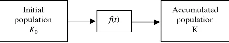
Figure 1.The structural scheme of the model of accumulation Another example concerns capital: under certain conditions, capital gives interests that, in their turn, together with the old capital provide new interests, etc. (Obi, 1998; Valakevičius, 2001).
The determined models of accumulation that dem-onstrate a non-linear function of accumulation will be further analysed in the paper. Fig.1 offers the structural scheme of the model of population accumulation that is constructed on the basis of the following equa-tion:
K
=
K
0f
(
t
)
.Initial population
K0
Let’s presume that K is the quantity of a certain product at the time moment t, and the rate of the prod-uct’s growth is the rate of the alteration of the function that relates the altering t and K. In other words, the rate of the product’s growth at every time moment is in portion to its quantity. Let’s also consider that the pro-portionality coefficient is constant and let’s mark it by the letter i. Then
K i dt dK
⋅
= . (1)
The result is an elementary differential equation with the differentiated variable quantities. The equation solved and the initial conditions estimated, i.e. when t = t0, the quantity of the product K is equal to its initial K0,
and when 0
0 K K
t= = , the expression of the quantity of
the product K is: t i
e
K
K
=
0⋅
⋅ . (2)If i is taken as the rate of interest and t is measured by the same time units as the time estimated in the in-terest rate, the equation (1) will show the natural expo-nential growth of the capital. To say more, this law is universal and may be applied for the modelling of other populations in order to both estimate their growth and vanishing (Rutkauskas, 2000).
Analogically, in the initial differential equation, let’s take the proportionality coefficient equal to the natural logarithm of any number r
(
r
>
0
,
r
≠
1
)
. Then,with r=1+i, the formula of compound percentage (i.e. of compound interest) is worked out:
( )
ti
K
K
=
0⋅
1
+
. (3)It is an exponential function. It should be also noted that, when t is a natural number, the equation (3) serves as a formula to calculate a certain member of the geo-metrical progression. During the modelling of the prod-uct’s growth by the given formula, it comes out that the product’s growth is infinite. In reality, the forecasting of the product’s increase in the distant future on the basis of this equation is inaccurate. At best, it may be used only in exceptional cases when the coefficient in the formula has been additionally corrected. No doubt, in-accurate financial forecasts may be explained by the imperfection of the formula (Misiūnas, 1997).
Logistic (i.e. limit) growth of the product
In the given case, the international term logistics is associated with the provision, i.e. with the possibility of the utilization of certain resources. As a rule, under naturally operating conditions, especially in a closed environment, the product cannot grow at equal rate. As has been mentioned it is particularly obvious in a closed system that possesses the necessary limited resources to maintain the growth of a particular product. As the ini-tial rate of the product’s increase gradually diminishes until considerable decline and total cessation, some-times such a system is said to be the system of the
lim-ited growth.
The phenomenon of the limited growth is frequently observed in nature. It is especially distinct in the animal populations expanded in a closed territory. As long as the population is relatively small and possesses substan-tial food resources and large space, the rate of its in-crease is great.
Contrariwise, when the population increases, it pos-sesses less and less space and food resources. Then the rate of its growth considerably diminishes (Tan-nenbaum, Arnold, 1995). A similar law of theso-called decreasing limit resultativity operating in the economic structures demonstrates that, in certain conditions, when the gross expenditure increases, the limit product (i.e. the rate of the product’s growth) decreases. In economic terminology, such peculiarity is called the limit capital efficiency. Here the limit efficiency is the rate of return, which is expected from additional investments. With the increase of the investment amount, the limit investment efficiency decreases. It is so because the initial invest-ments have been realized at the most favourable condi-tions, which caused large rates of income. Meanwhile, later investments are not so much effective and offer evenly smaller income (Pass, 1997, and others).
The operation of the mentioned law is especially obvious in agriculture. If initially, for the cultivation of the plot of constant size (for instance, one thousand hectares) only several workers are employed, and later their number considerably increases, after some time the limit work product (i.e. the rate of the work product’s growth) will start decreasing. Economic literature main-tains that the situation to be otherwise, the entire world might be nourished from the mentioned single plot (Wonnacott P., Wonnacott R., 1998). Undoubtedly, if the exponential law of growth operated all the time, the product’s growth were unlimited and, during a long period, its manufacturing would grow to a desirable extent of amount.
Nevertheless it should be noted that, in most cases, the term limit employed in the theory of economics possesses another value, that is the value of rate, since it is associated with the mathematical derivative of the function estimating a certain phenomenon. The derivative is found out by the calculation of the limit (Van Horne, 1995).
Logistic (i.e. limit) future value of the product
As far ago as the 19th century, when investigating the alteration of the biological systems, P.F. Verhülst suggested to supplement the differential equation of the growth of population with the multiplier possessing the shape of a linear decreasing function:
m
K
K
−
1
; (4)where Km is the maximum (limit) value of the bio-logical population or of any other product expressed by the units estimating its amount.
the natural logarithm of any number r
(
r
>
0
,
r
≠
1
)
. Theestimation of the initial conditions and the solution of the differential equation with respect to the product K results in the logistic (limit) future value of the product:
(
1)
0 0
− +
⋅ ⋅ =
t m
t m
r K K
r K K
K .
Here, presuming that r=1+i, the following for-mula is obtained:
(
)
(
)
(
1 1)
1 0
0 − + +
+ ⋅ ⋅
= t
m
t m
i K K
i K K
K . (5)
It is the logistic (limit) future value of the product expressed by the rate of the growth percentage (Girdzi-jauskas, 2002).
Having divided both the nominator and the denomi-nator of the equation’s (9) right part by Km and marked the ratio
m
K
K0 by the letter S
0
≤ ≤
= 0, 0 0 1
0
S S K K
m
, let’s
consider this ratio the coefficient of the initial conges-tion. In order to ascertain that time will be measured by the same units as the time estimated in the rate of the growth percentage, let’s mark it by the letter n that, most frequently, expresses the entire periods of the per-centage rate re-calculation. Thus re-worked, the future value of the limit alteration is:
( )
( )
(
1 1)
1 1 0
0
− + ⋅ +
+ ⋅
= n
n
i S
i K
K . (6)
The function of the product’s logistic accumulation has been obtained, which demonstrates the relative ex-pression, in other words, the coefficient of initial con-gestion.
It is important to maintain that, in case the product’s maximum value Km increases and approaches infin-ity
(
Km →∞)
, the coefficient of the initial congestiondeclines and its value approaches zero
(
S0 →0)
. Then, as one could expect, the formula (6) is no more than a conventional formula of compound percentage (3). The same will be obtained by having calculated the limit for the equation (5) whenKm→∞. On the other hand, if inthe equation (6)K0 =Km, i.e. the initial product is equal to its maximum value, then the coefficient of the initial congestion S0 will be equal to 1. When in the equation (6) S0 = 1, the result is the conclusion confirm-ing the initial condition:K0 =Km.
Thus, the formula of compound percentage makes a separate case of the logistic function of accumulation when the maximum value of the product Km is im-mensely large.
It should be also stressed that the obtained logistic function differs from the classical one whose expression is as follows:
1
)
(
+
⋅
=
⋅⋅
x x
e
e
K
x
K
λλ
or
x
e
K
x
K
− ⋅+
=
λ1
)
(
. (7)The latter function is defined in the entire set of real numbers and undergoes alteration within the interval (0; K). In other words, all the values of the function have been distributed between two horizontal lines K(x) = 0 and K(x) = K. Externally, the central part of the graph of the logistic function resembles a deformed Latin „S“. The authors claim that, with the increase of the argu-ment (i.e. time), the function (i.e. product) approaches the constant value equal to the quantity of the coeffi-cient K. This peculiarity is the most essential for further generalizations. Fig.2 presents the graphs of this func-tion when the coefficient K is constant and the values λ
are different. With the increase of the coefficient λ when
the argument is in the environment of zero, the rate of the function’s growth further enlarges:
0 0,2 0,4 0,6 0,8 1
-30 -20 -10 0 10 20 30
Duration of accumulation
P
ro
du
ct
K=1; λ=0,1 K=1; λ=0,2 K=1; λ=0,5
Figure 2. The graph of the logistic function
The alteration of the logistic function when the ar-gument x is close to zero resembles the diagram of the exponential function (2). The authors maintain that, in this case, there is no direct relation between the expo-nential and logistic functions since there is no direct passage from one type of dependency to another.
Moreover, all the functions of the limited growth whose character of alteration is similar to the alteration of the logistic function (7) are also called logistic. The logistic functions of the type of the formula (6) that are more fit for the modelling of the financial phenomena will be discussed further as well as the possibilities of the exponential and logistic function application.
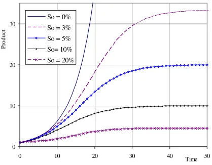
Let’s compare the diagrams of the exponential (7) and logistic (6) accumulation (i.e. the graphs of the fu-ture values). Fig. 3 presents the diagrams that illustrate the dependency of the product‘s future value on time. Here the interest rate of the graphically illustrated func-tions makes 20% and the initial congestion S0 alters from 0 to 20% (i.e. the exponential variant shows the absence of congestion). At the initial moment, the prod-uct’s value is equal to one (K0 = 1). It means that the initial product is equal to one and that other values are expressed by the initial product.
conges-tion coefficient, the product’s future value decreases despite other parameters of the logistic function remain-ing unchanged.
0 10 20 30
0 10 20 30 40 Time 50
Pr
od
uc
t
So = 0% So = 3% So = 5% So= 10% So = 20%
Figure 3.The product's dependency on time when the values of the initial congestion are various
and when i=0,2, Ko=1
The diagram shows that, at the beginning (when n values are low), all the functions (logistic and conven-tional) do sufficiently overlap. To say more, a rather inconsiderable value difference (e.g. about 5%) remains for a longer period in case the percentage rate is smaller. Later on the rise of the limit function graphs slackens until its complete cessation.
The mentioned peculiarity of the diagram can be easily observed in the analytical investigation of the logistic function. The search for K
n→∞
lim leads to the finding the indeterminacy
∞
∞
. Here the application of the Liopital’s rule results in the following:( )
( )
(
)
(
( ) ( )
( ) ( )
n)
mn
n n n
n S K
K i i S
i i K i
S i
K = =
− + + +
+ + =
− + +
+
∞ → ∞
→ 0
0
0 0
0 0
0 1 ln 1 0
1 ln 1 lim 1 1 1
1 lim
It should be noted that the semblance of value at the initial moment graphically illustrates the fact discussed above, i.e. the exponential function (3) making a sepa-rate case of the logistic function (6).
Limit interest
It is time to discuss a particular product, i.e. capital, and its increase in a certain period of time, i.e. interest. The compound interest as well as the limit interest point to the difference between the accumulated capital K and the initial capital K0:
0 K K
P= − ,
where P is the interest accumulated during a certain period.
The expression of the future capital value of the limit alteration (5) allows for the following:
(
)
(
)
(
)
00 0
1 1
1
K i
K K
i K K P
t m
t
m −
− + +
+ ⋅ ⋅
= .
Then:
(
) (
(
)
)
(
)
(
1 1)
1 1
0 0 0
− + −
− + −
= n
m
n m
i K K
i K K K
P .
The numerator and the denominator having di-vided by Km, the result is:
(
) (
(
)
)
(
)
(
1 1)
1
1 1
1 0 0 0
− + +
− + −
= n
n
i S
i S K
P . (8)
Another division by
(
(
1+)
n −1)
i marked as follows:
(
)
n uni
= −
+ 1
1
1 leads to such expression of the limit
in-terest:
0 0 0
1
S u
S K P
n+
−
= .
When the congestion S0 is constant, the quantity of interest depends on the accumulation factor un, which, in its turn, is the function of the interest rate and accu-mulation duration. It decreases both with the increase of the interest rate and of accumulation time. The quantity of the interest also has its limit, which is equal toK0
(
1−S0)
S0.Application of limit accumulation models
Practically, the problem of the logistic (limit) accu-mulation of the capital has not yet been investigated. It was determined by several important reasons. First of all, no adequate models have been worked out. Obvi-ously, the logistic models are much more complete than the exponential ones and therefore their analysis is pos-sible only with the invocation of information technolo-gies. Finally, the logistic models should be mostly ap-plied for the closed economic systems; however, the mentioned condition is fully realized rather rarely.
The statistic analysis of the long-term economic de-velopment of some systems allows for the conclusion that, in certain periods, there exist the indications point-ing to the fact of approachpoint-ing a certain limit. Such con-clusions are found in scanty publications on the men-tioned problem (Ferreira, Eidelman, 1998).
Let’s consider the case of the economic structure in Brazil. For a long time, it was isolated from external resources. Carlos Feu Alvim based his analysis of the GDP in Brazil in 1947-1992 on this very fact. By having employed the phenomenological methodology and based his research on the analysis of the national indi-ces, the author arrived at the conclusion that, at the end of the investigated period, the accumulated capital hardly reaches 7% of the value, which was prognosed by the exponential model. In 1998 another more pro-found investigation was carried out by employing simi-lar methodology and operating with new additional data (until 1997).
factor that limited the growth of Brazil’s economic level (here manpower was not sufficiently exploited). The given conclusion is that up to the seventh decade the economic structure of Brazil may be described by the logistic model, which reveals that the rate of the eco-nomic growth is stemmed by the limit capital. The re-searchers offered an insignificantly modified variant of the classical logistic function (7). It goes without saying that the employment of the logistic function (6) brings more precise forecasting results.
Determination of the regression coefficients
In the application of the logistic models of accumu-lation, the determination of the regression coefficients comes to be one of the most important and problematic tasks.
Let’s define the conditions under which one model of capital accumulation (CAM) might be replaced by another, i.e. more elementary model. When the maxi-mum value of the capital limits its growth insignifi-cantly, the exponential analytic model may be em-ployed. As has been observed above, the values calcu-lated by both models at the beginning of the growth period are rather close. It has been also noted that the exponential model solely makes a separate case of the logistic model. Therefore having the time line of the values of the capital and knowing that the variable quantities operate according to the law of the limit growth allows for the description of the initial values of the time line by the exponential model. Furthermore, the coefficients of the latter model may be used in the con-struction of the logistic model.
By applying the above mentioned conclusions, the logistic model coefficients K0 and i will be calculated with the help of the lowest square method and according to the exponential model (Boguslauskas, 2004). The expression of the exponential CAM y = a(1+i)x will serve as the regression equation:
1
)
1
(
ˆ
1 xi
a
y
=
+
,2
) 1 (
ˆ2 x
i a
y = + ,
...
n
x
n
a
i
y
ˆ
=
(
1
+
)
.The lowest square method allows for the description of the differences between the theoretical and experi-mental values and for the structuring of the sum of de-viation squares:
2 2
2 2 2 1
1 ) (ˆ ) ... (ˆ )
ˆ
(y y y y yn yn
u= − + − + + −
By having inserted the modelled y values of the de-viations and replaced (1+i) by r (1+i = r) the function is described as follows:
2 2
2 2
1) ( ) ... ( )
( 1 2
n x x
x y a r y a r y
r a
u= ⋅ − + ⋅ − + + ⋅ n − (11)
The function (11) possesses two variable quantities, i.e. a and r.
Let’s apply the obtained function to the calculation of the regression coefficients in the solution of a par-ticular problem. Table 1 presents the dynamics of the GDP in Lithuania in 1992-2003 (in mln Lt; Department of Statistics, 2004). The data of the period from 1992 to 1995 is taken for the determination of the coefficients of the exponential function:
Table
Lithuania’s GDP in 1992-2003
Years 1992 1993 1994 1995 1996 1997
GDP 3406 11590 16904 25568 32290 39378
Years 1998 1999 2000 2001 2002 2003
GDP 44377 43359 45526 48379 51633 55737
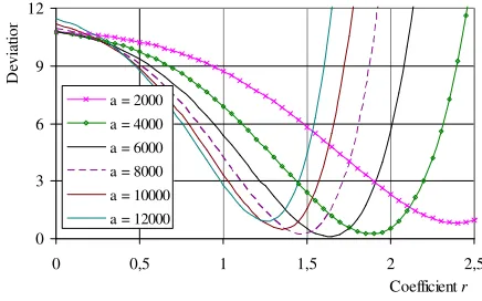
Relying on the mentioned data of the initial four years, Fig.4 shows the dependency of the sum of devia-tion squares on the growth rate coefficient r at different a values. Fig. 4 demonstrates that this function has its minimum when r is between 1.5 and 2.0 and a is close to 6000.
0 3 6 9 12
0 0,5 1 1,5 2 2,5
Coefficient r
D
ev
ia
tio
n
a = 2000 a = 4000 a = 6000 a = 8000 a = 10000 a = 12000
Figure 4. The dependency of the sum of deviation squares on the growth rate coefficient r
at different a values
In order to find out the precise minimum of the func-tion as well as the coefficients in-search it is necessary to calculate the function’s derivatives with respect to sepa-rate variable quantities and to equate them to zero.
The calculation of the derivatives leads to the fol-lowing:
⋅
⋅
⋅
−
⋅
⋅
+
+
⋅
⋅
⋅
−
⋅
⋅
+
+
⋅
⋅
⋅
−
⋅
⋅
=
∂
∂
⋅
−
⋅
⋅
+
+
⋅
−
⋅
⋅
+
⋅
−
⋅
⋅
=
∂
∂
− − −
.
)
(
2
...
...
)
(
2
)
(
2
;
)
(
2
...
...
)
(
2
)
(
2
1 1 1 2
1 1 1
2 1
2 2
1 1
2 2
1 1
n n
n n
x n n x
x x
x x
x n x
x x
x x
r
x
a
y
r
a
r
x
a
y
r
a
r
x
a
y
r
a
r
u
r
y
r
a
r
y
r
a
r
y
r
a
a
u
solu-tions of the system:
=
∂
∂
=
∂
∂
,
0
;
0
r
u
a
u
. The rearrangements and
the solution of each equation of the system with respect to the unknown quantity result in:
⋅
⋅
⋅
=
⋅
=
∑
∑
∑
∑
= = = =.
)
(
)
(
;
)
(
1 2 1 1 2 1 n j x j n j x j j n j x n j j x j j j jr
x
r
y
x
a
r
y
r
a
The equalization of the equations’ right parts and certain slight modifications lead to the following:
0 ) ( ) ( ) (
1 1 1 1
2 2 = ⋅ ⋅ ⋅ − ⋅ ⋅ ⋅
∑
∑
∑
∑
= = = = n j n j n j x j j n j x x j jxj j j j
r y x r r x y
r (12)
The analytical solution of this equation is rather complicated, especially when n is considerably higher than 2.0. The most convenient way of its solution is found in the use of information technologies. The au-thors see one of such solutions in the creation of the iteration cycle during which the value of the regression coefficient is altered until it satisfies the formed equa-tion at necessary precision.
The solution of the obtained equation and the find-ing of the coefficient allows for the calculation of the second regression coefficient a. The value of the coeffi-cient a is determined due to one of the system’s equa-tions. In the analysed example, the values are as fol-lows: r = 1.628714 and a = 6049.49.
In the estimation of the obtained values of the coef-ficient, the specificity of the problem should be accen-tuated. In fact, the statistic data reflects the situation of the transitional economic period. On the other hand, the values of the regression coefficients r and a depend not only on the statistic data acquired during particular ob-servations but also on the number of the observed ele-ments employed in the concrete calculation.
When possessing the necessary r and a coefficients, it is important to determine the final logistic model’s coefficient Km. Let’s define K = Y, and Km = z. As be-fore, let’s presume that 1 + i = r and K0 =a. Then the logistic function of accumulation will read as follows:
)
1
(
−
⋅
+
⋅
⋅
=
xxr
a
z
r
z
a
Y
.From this it is found out that the values of the
func-tion conforming to the arguments x1,x2,...,xn are:
)
1
(
ˆ
1 11
+
⋅
−
⋅
⋅
=
x xr
a
z
r
z
a
Y
)
1
(
ˆ
2 22
+
⋅
−
⋅
⋅
=
x xr
a
z
r
z
a
Y
...)
1
(
ˆ
−
⋅
+
⋅
⋅
=
n n x x nr
a
z
r
z
a
Y
The unknown regression coefficient z may be calcu-lated by employing the lowest square method:
2 2 2 2 2 1
1
)
(
ˆ
)
...
(
ˆ
)
ˆ
(
Y
Y
Y
Y
Y
nY
nv
=
−
+
−
+
+
−
Finally, by inserting the modelled values of the variable quantities the required function is obtained:
.
)
)
1
(
(
...
)
)
1
(
(
)
)
1
(
(
2 2 2 2 1 2 2 1 1 n x x x x x xY
r
a
z
r
z
a
Y
r
a
z
r
z
a
Y
r
a
z
r
z
a
v
n n−
−
⋅
+
⋅
⋅
+
+
+
−
−
⋅
+
⋅
⋅
+
+
−
−
⋅
+
⋅
⋅
=
In order to discover the minimum of the function it is necessary to calculate the function’s derivate accord-ing to z and to equalize it to zero:
+
−
⋅
+
−
⋅
⋅
⋅
−
−
⋅
+
⋅
⋅
⋅
=
2 2 1))
1
(
(
)
1
(
)
)
1
(
(
2
1 1 1 1 1 x x x x xr
a
z
r
r
a
Y
r
a
z
r
z
a
dz
dv
+ + − ⋅ + − ⋅ ⋅ ⋅ − − ⋅ + ⋅ ⋅ ⋅ + ... )) 1 ( ( ) 1 ( ) ) 1 ( ( 2 2 2 2 2 2 2 2 2 x x x x x r a z r r a Y r a z r z a.
0
))
1
(
(
)
1
(
)
)
1
(
(
2
2 2=
−
⋅
+
−
⋅
⋅
⋅
−
−
⋅
+
⋅
⋅
⋅
+
n n n n n x x x n x xr
a
z
r
r
a
Y
r
a
z
r
z
a
Insignificant modifications allow for a reduced ex-pression of the equation:
∑
==
−
⋅
+
−
⋅
⋅
⋅
−
−
⋅
+
⋅
⋅
n j x x x j x x j j j j jr
a
z
r
r
a
Y
r
a
z
r
z
a
1 2 20
))
))
1
(
(
)
1
(
(
)
)
1
(
((
In order to find out the regression coefficient z the equation must be solved and the value z, by which the equation is satisfied, must be obtained. It is convenient to solve such an equation with the help of the digital method. Digital methods are iteration procedures where the results achieved during each step are compared with the earlier achieved ones to choose the best solution.
optimal.
The data of the time line used for the determination of the coefficient z also embraces the data employed for the determination of the coefficients a and r. In other words, the latter data overlaps with the former. Then the obtained coefficients important for the statistics of the GDP in Lithuania are inserted into the logistic regres-sion equation:
(
1
,
629
1
)
5
,
56877
5
,
56877
629
,
1
49
,
6049
5
,
56877
−
⋅
+
⋅
⋅
=
tt
K
.The statistic data of the GDP and the logistic regres-sion curve are presented in Fig. 5:
0 20 40 60
0 2 4 6 8 10 12
Yars
G
D
P
(m
ln
L
t)
GDP in Lithuania
Logistic curve
Exponential curve
Figure 5. Regression curves of Lithuania's GDP
Fig. 5 also shows the operation of the exponential function obtained on the basis of the initial data:
t
,
K
=
6049
489
⋅
1
,
629
.It apparently demonstrates that the forecasting di-rected into the remote future causes considerable devia-tions (e.g. in the middle of the interval, the error ex-ceeds 100%).
Conclusions
Logistic (limit) models are applied for the investiga-tion of the alterainvestiga-tion of some kinds of populainvestiga-tion. The majority of populations, especially capital, distinguish by their reproductivity, i.e. the capacity to get restored, to renew, and expand (multiply). In the case of the capi-tal, it manifests itself in the interest that participates in the creation of the capital of new generation (together with the initial capital). Therefore, until restrictions do not occur, it might be considered that the capital is growing in a constant rate. The exponential models are used for the modelling of the alteration of the perma-nently growing product. However, such models are not always sufficiently precise and convenient for practical use. The analysis of the models of accumulation has lead to the following conclusions:
• The logistic models allow for the modelling of
the development of the populations whose growth is limited by the insufficiency of resources. The
logistic models of accumulation reflect the dy-namics of the population’s (capital’s) growth more precisely;
• The exponential model makes a separate case of
the logistic (limit) model;
• The expression of capital in a closed system
demonstrates the slackening character and has its limit equal to its maximum value;
• The lowest square method used to determine the
regression coefficients may be applied gradually. For this purpose, it is convenient to employ the exponential function as a separate case of the lo-gistic function;
• The logistic models may be used in the
construc-tion of the regression coefficient of a particular object.
Such proposition is worked out on the logistic re-gression equation of the GDP in Lithuania that was made on the basis of the statistic data from twelve latter years.
References
1. Bodie, Z. Finance/ Z. Bodie, R. C. Merton. New Jersey, 2000.
586 р.
2. Bodie, Z. Essentials of Investments / Z. Bodie, A. Kane, A.J.
Marcus. McGraw-Hill, 2000. 984 p.
3. Bubnys, E. Įmonės finansų valdymas. Kaunas: Technologija,
1997. 220 p.
4. Buškevičiūtė, E. Finansų analizė/ E. Buškevičiūtė,
I. Mačerinskienė. Kaunas: Technologija, 1998. 380p.
5. Pass, Ch. Ekonomikos terminų žodynas / Ch. Pass, B. Lowes, L.
Davies. Vilnius: Baltijos biznis, 1997, 584 p.
6. Edvards, C.H., Penney D. E. Elementary Differential Equations
with Applications / C.H. Edvards, D. E. Penney. New Jersey, 1985. 632 p.
7. Gaidienė, Z. Finansų valdymas. Kaunas: Pasaulio lietuvių
kul-tūros, mokslo ir švietimo centras, 1995. 112 p.
8. Girdzijauskas, S. Finansiniai skaičiavimai. Kaunas:
Tech-nologija,1997. 178 p.
9. Girdzijauskas, S. Draudimas: kiekybinė finansinė analizė.
Kau-nas: Naujasis lankas, 2002. 104 p.
10. Girdzijauskas S. Kapitalo kaupimo logistiniai modeliai: VU
Kauno humanitarinio fakulteto konferencijos ”Informacinės
tech-nologijos verslui – 2002“ pranešimų medžiaga. Kaunas:
Tech-nologija, 2002, p. 40-44.
11. Girdzijauskas, S. Evaluierung der Zinsnorm in Grenzmodellen:
The Materials Scientific International Conference “Integration of Market Economy Countries: Problems and Prospects”. Riga, May 27–28/2003, /Higher School of Economics and Culture, p. 19-26.
12. Girdzijauskas, S. Logistiniai (ribiniai) kaupimo modeliai//
Informacijos mokslai, 2002, t. 23, p. 95-102.
13. Katauskis, P. Finansų matematika. Vilnius: LB, 1997. 168 p.
14. Kubilius, J. Tikimybių teorija ir matematinė statistika. 2-asis
patais. ir papild. leid. Vilnius: VU leidykla, 1996. 440 p.
15. Obi, C.P. Verslo finansų pagrindai. Kaunas: Technologija,
1998. 298 p.
16. Omar Campos Ferreira. Capital Accumulation in the Brazilian
Economy. Economy and Energy, Year II-No9, July/August/1998.
17. Rutkauskas, A.V. Finansų ir komercijos kiekybiniai metodai.
Vilnius: Technika, 2000. 504 p.
Rut-kauskas, V. Damašienė. Šiauliai: Šiaulių universiteto leidykla, 2002. 248 p.
19. Schall Lawrence D., Haley Charles W., Schachter Barry.
Intro-duction to Financial Management. Toronto: McGraw-Hill Ryer-son Limited, 1981.
20. Sharpe, W.F. Investments / W.F. Sharpe, G.J., Alexander, J.V.
Bailey. Prentice Hall International, Inc.1999. 1028 p.
21. Department of Statistics at the Government of the Republic of
Lithuania. Statistic Data of the GDP in Lithuania [interactive]. The document renewed on 29 July 2004 [examined on 25 August
2004] <http://www.std.lt/web/main.php?parent=1025>
22. Šakys, V. SkaičiuoklėMicrosoft Excel 97 firmos vadybai.
Kau-nas: PIF, 1998. 496 p.
23. Tannenbaumas, P. Kelionė į šiuolaikinę matematiką / P.
Tannenbaumas, R. Arnoldas. Vilnius: TEV, 1995. 512 p.
24. Valakevičius, E. Investicijų mokslas. Kaunas: Technologija,
2001. 324 p.
25. Van Horne, J. C. Fundamentals of Financial Management. New
Jersey: Prentice Hall, 1995. 800 p.
26. Vince, R. The Mathematics of Money Management. New York:
Jon Wiley & Sons, Inc., 1998. 400 p.
27. Wonnacott, P. Mikroekonomika / P. Wonnacott, R. Wonnacott.
2–asis patais. leid. – Kaunas: Poligrafija ir informatika, 1998. 572 p.
28. Интрилигатор, М. Математические методы оптимизации и экономическаятеория. Москва: АЙРИСПРЕСС, 2002. 566 c. 29. Ковалев, В.В. Курс финансовыхвычислений/ В.В. Ковалев,
В.А. Уланов. Москва: Финансыистатистика, 1999. 328 c. 30. Колемаев, В.Ф. Математическая экономика. Москва:
ЮНИТИ-ДАНА, 2000. 400 c.
31. Малыхин, В.И. Финансовая математика. Москва: ЮНИТИ
-ДАНА, 2000. 246 c.
32. Мелкумов, Я.С. Финансовыевычисления. Теорияипрактика.
Москва: ИНФРА-М, 2002. 384 c.
33. Мертенс, А. Инвестиции. Киев: Киевское инвестиционное агенство, 1997. 416 c.
34. Мышкис, А. Элементы теории математических моделей.
Москва: ЕдиториалУРСС, 2004. 192 c.
35. Четыркин, Е.М. Финансовый анализ производственных инвестиций. Москва: ДЕЛО, 1998. 256 c.
Stasys Girdzijauskas, Vytautas Boguslauskas
Logistinių kaupimo modelių taikymo galimybės
Santrauka
Dauguma besivystančių populiacijų, priklausomai nuo jų
prigim-ties, naudoja kokius nors išteklius. Ištekliai savo ruožtu, priklausomai
nuo jų santykio su pačia populiacija, gali būti tiek baigtiniai, tiek
begaliniai. Logistiniai kaupimo modeliai yra paremti senkančių
ištek-liųįtaka populiacijos augimo procesui. Išteklių ribotumas, savo
pri-gimtimi būdamas vienas svarbiausių daugelio sistemų vystymosi
veiksnių, dažnai per menkai vertinamas, ir Tai yra ne tik dėl to, kad
dauguma išteklių yra sunkiai išmatuojami, bet ir dėl to, kad, trūkstant
patikimų ir patogių prognozavimo priemonių, kartais neįmanoma net
apytikriai numatyti rezultatus.
Darbe sutelktas dėmesys į specifines populiacijas, t.y.
populiaci-jas, gebančias augti natūraliai, į tokias, kurios augdamos pačios
duo-da pagal tą patį principą didėjantį prieaugį. Natūralus augimas – tai toks augimo greitis, kai kiekvienu laiko momentu jis proporcingas
populiacijos dydžiui: kuo didesnė populiacija, tuo ji greičiau auga.
Tokioms populiacijoms gali būti priskiriamas kapitalas, pinigų srautai
ar kitas panašias savybes turintis produktas. Tai leidžia užrašyti
paprastas diferencialines lygtis, įgalinančias sudaryti patogius
popu-liacijų vystymosi modelius.
Jei K – tam tikro produkto dydis laiko momentu t, o to produkto
augimo greitis yra kintamuosius t ir K siejančios funkcijos kitimo
greitis, tai, laikydami, kad kintamuosius sieja proporcingumo
koefi-cientas i, gausime, kad dK dt=i⋅K. Išsprendę šią lygtį ir įvertinę
pradines sąlygas, kad laiko momentu t = t0 produkto dydis K lygus
pradinei jo reikšmei K0, randame produkto kiekio K išraišką
t i
e K K= 0⋅ ⋅.
Tuo pačiu principu galima sudaryti ir išteklių ribotumą į
verti-nančius augimo (logistinius) modelius. Logistinių modelių yra į
vai-rių. Kai kurie jų plačiai taikomi biologinių sistemų tyrimui. Tačiau
ekonominių reiškinių nagrinėjimui šie modeliai sunkiai pritaikomi. Jų
trūkumas – nėra natūralaus perėjimo į sudėtinių procentų išraišką.
Statistiškai nagrinėjant kai kurių sistemų ilgalaikį ekonominį
vystymąsi, pastebėta, kad atskirais periodais egzistuoja artėjimo prie
tam tikros ribos požymiai. Izoliuotoje aplinkoje platesnės apimties
ekonominį eksperimentą atlikti yra sudėtinga, todėl teko nagrinėti
pasaulinę patirtį, ieškoti realių praktinių pavyzdžių. Žinoma, kad
Brazilijos ekonomika ilgą laiką buvo izoliuota nuo išorinių išteklių.
Įvertinus tą faktą, Karlas Alvimas (Carlos Feu Alvim) ir Omaras
Fereira (Omar Compos Ferreira) atlikto Brazilijos BVP augimo
tyri-mus. Naudodami fenomenologinę metodologiją ir remdamiesi
nacio-nalinių rodiklių analize, autoriai priėjo išvadą, kad laikotarpio
pabai-goje sukauptasis kapitalas siekia vos 7 proc. tos reikšmės, kuri buvo
prognozuojama remiantis rodikliniu modeliu. Buvo ieškoma struktū
-rinių “Brazilijos ekonominio stebuklo” pabaigos priežasčių.
Pagrin-dinė hipotezė ta, kad ekonomikos augimą ribojantis veiksnys yra
kapitalas (darbo jėga Brazilijoje buvo išnaudojama ir taip
nepakan-kamai). Taigi čia prieinama išvada, kad nagrinėjamo laikotarpio
ekonomika gali būti aprašoma logistiniu modeliu, kur augimo tempą
stabdantis veiksnys yra ribinis kapitalas. Kapitalo augimo
modelia-vimui tyrimo autoriai siūlė mažai modifikuotą klasikinės logistinės
funkcijos variantą.
Šiame darbe naudojamas patobulintas logistinis augimo modelis. Jis turi pertvarkytus koeficientus ir yra bendriausias tokio tipo
popu-liacijų augimo modelių atvejis:
( ) ( )
(
1 1)
1
0 0
− + +
+ ⋅ ⋅
= t
m
t m
i K K
i K K
K
(čia K0 – pradinė populiacija, išreikšta jos kiekį įvertinančiais
vienetais, Km – maksimali (ribinė) populiacijos reikšmė, i – augimo
norma, t – augimo trukmė, išreikšta tais pat laiko vienetais kaip ir
augimo laikas). Plačiai iki šiol kapitalo augimui modeliuoti taikyta
sudėtinių procentų taisyklė ( )t
i K
K= 0⋅1+ yra atskirasis šio logistinio modelio atvejis. Parodoma, kad tipinė matematinėje analizėje varto-jama logistinė funkcija
(
x)
m e K
K= 1+ −λ skiriasi nuo nagrinėjamos funkcijos ir nėra šios funkcijos kuris nors atskirasis atvejis. Reikia pažymėti, kad mūsų siūlomas patobulintas logistinis augimo modelis duoda tikslesnius prognozės rezultatus, nei klasikinis.
Vienas svarbiausių sistemos augimo rodiklių yra per tam tikrą laiką sukauptos palūkanos. Logistinis modelis taip pat leidžia apskai-čiuot tokias palūkanas. Ribinės palūkanos P yra sukauptojo K ir pradinio K0 kapitalų skirtumas:
0
K K P= − .
Sutrumpinta tokių palūkanų išraiška yra
0 0 0 1
S u
S K P
n+ −
= ,
kur
m K K
S0= 0 – pradinio prisotinimo koeficientas, o
(
)
(
1 1)
1 + −
= n
n i
u . Esant pastoviam prisotinimui S0, palūkanų dydis priklauso nuo kaupimo veiksnio un, kuris savo ruožtu yra palūkanų normos ir kaupimo trukmės funkcija. Jis mažėja, tiek didėjant palūkanų normai, tiek kaupimo laikui. Palūkanų dydis taip pat turi ribą, lygią
(
0)
0 01 S SK − .
meto-das. Uždavinio sprendimo sunkumas tas, kad šis modelis yra netiesi-nis ir turi ne mažiau kaip tris neapibrėžtus koeficientus: K0, Km ir i. Todėl mažiausių kvadratų metodą logistinio modelio regresijos koefi-cientams nustatyti siūloma taikyti palaipsniui. Pradiniu laiko momen-tu populiacijos reikšmės, apskaičiuotos remiantis logistiniu ir ekspo-nentiniu modeliu, yra labai artimos. Todėl patogu, panaudojus atski-rąjį logistinės funkcijos atvejį – eksponentinę funkciją, nustatyti pradinius logistinės funkcijos koeficientus: pradinį populiacijos dydį
K0 ir augimo greičio koeficientąi. Toliau, įrašius šiuos duomenis į bazinę išraišką, nesudėtinga apskaičiuoti ir ribinę (didžiausią) popu-liacijos reikšmę.
Teorinių apibendrinimų teisingumas pagrindžiamas konkretaus objekto regresijos lygties sudarymu. Tam panaudojami 1992–2003 metų Lietuvos BVP statistiniai duomenys. Pirmiausia eksponentinės funkcijos koeficientams nustatyti imami pirmųjų ketverių metų duo-menys. Jais remiantis, sudaryta nuokrypų kvadratų sumos priklauso-mybė nuo augimo greičio koeficiento, esant skirtingoms pradinėms populiacijos reikšmėms. Įsigilinę pastebime, kad ši funkcija turi minimumą, esantį tarp 1,5 ir 2, kai pradinė populiacija yra artima 6 000. Ieškant tikslaus šios funkcijos minimumo, apskaičiuojamos funkcijos išvestinės atskirų kintamųjų atžvilgiu ir jos prilyginamos nuliui. Palyginę dešiniąsias lygčių puses ir atlikę nežymius pertvar-kymus, gauname šią lygtį:
0 ) (
) ( ) (
1 1 1 1
2 2
= ⋅ ⋅ ⋅ − ⋅ ⋅ ⋅
∑
∑
∑
∑
= = = =
n
j
n
j
n
j
x j j n
j x x
j j
xj j j j
r y x r
r x y
r .
Analitinis šios lygties sprendimas yra gana keblus, ypač kai laipsnio rodiklis n daug didesnis nei 2. Patogiausia tokius uždavi-nius spręsti naudojantis informacinėmis technologijomis. Vienas iš galimų sprendimo būdų – iteracinio ciklo sudarymas, kurio metu kiekvienoje iteracijoje keičiama vieno iš regresijos koeficientų reikšmė tol, kol ji galiausiai reikiamu tikslumu atitinka sudarytąją lygtį. Antrojo koeficiento reikšmė nustatoma išsprendus vieną iš
pradinės sistemos lygčių, kurioje pirmojo koeficiento reikšmė jau yra žinoma. Tokiu būdu mūsų nagrinėjamame pavyzdyje šios reikšmės yra: augimo greičio koeficientas – 1,628714, o pradinio kapitalo reikšmė – 6049,49 mln. litų.
Turint minėtus du koeficientus, apskaičiuojamas ir paskutinis logistinio modelio koeficientas Km. Jis randamas, logistinės lygties išvestinę prilyginus nuliui
∑
=
= − ⋅ +
− ⋅ ⋅ ⋅ − − ⋅ +
⋅ ⋅ n
j
x x x
j x
x
j j j j
j
r a z
r r a Y r
a z
r z a
1 2
2
0 )) )) 1 ( (
) 1 ( (
) ) 1 ( ((
Ir ankstesniųjų, ir šios lygties sprendimui taikome apytikslius metodus. Atlikę reikalingus apskaičiavimus, gauname, kad paskuti-niojo koeficiento reikšmė yra 6049,49.
Tada logistinis Lietuvos BVP augimo modelis būtų:
(
1,629 1)
5 , 56877 49 , 6049
629 , 1 49 , 6049 5 , 56877
− ⋅ +
⋅ ⋅
= tt
K .
Vertinant gautąsias koeficientų reikšmes reikia pabrėžti užda-vinio specifiką: statistiniai duomenys atspindi pereinamojo ekono-minio laikotarpio situaciją. Kita vertus, regresijos koeficientųK ir i
reikšmės priklauso ne tik nuo statistinių duomenų, gautų atskirų stebėjimų metu, bet ir nuo stebinių skaičiaus, panaudotų konkre-čiame skaičiavime.
Apibendrinant daroma išvada, kad logistiniai kaupimo modeliai tiksliau atspindi populiacijos (kapitalo) augimo dinamiką ir gali būti taikomi ten, kur reikia įvertinti senkančius išteklius. Eksponentinis modelis yra tik atskiras logistinio modelio atvejis. Mažiausių kvadra-tų metodą logistinio modelio regresijos koeficientams nustatyti gali-ma taikyti palaipsniui.
Raktažodžiai: populiacija, produktas, modelis, senkantys ištekliai, sudėtinės palūkanos, logistinis augimas, būsimoji vertė, mažiausių kvadratų metodas, regresijos lygtis, bendrasis vidinis produk-tas (BVP)