The Economic Impact of Remittances and Foreign Trade on Migration.
Granger-Causality Approach
Dominik Metelski, Antonio Mihi-Ramirez
University of Granada
Campus Cartuja s/n, 18071, Granada, Spain E-mail. [email protected], [email protected]
http://dx.doi.org/10.5755/j01.ee.26.4.12464
This paper analyzes the bidirectional relationship between several mobility factors such as migration, remittances and foreign trade.
The issue that certain mobility factors might be substitutes was first raised by economists Heckscher and Ohlin and was later picked up several times by other authors in the literature. We assumed that such a debate should be revived and addressed again, especially having in mind growing importance of mobility factors in contemporary economies.
Using modern and sophisticated econometric technique such as Granger-causality analysis we studied the case of Spain taking yearly data from 1975 till 2013. The autoregression vector model was used as well as Granger-causality test was employed to provide evidence that such a reciprocal type of relationships between the economic factors subject of our study in reality exist.
The results of Granger-causality test have led us to the conclusion that export causes migration and also migration causes export. Results also showed that net migration and international trade are treated as substitutes. Further, we found that not only migration causes higher remittances, which is consistent with an intuitive feel, but also past remittances draw further migration.
In terms of the Heckscher-Ohlin model, the enormous growth of migration flows in the contemporary time is explained partly because progressive reduction of costs has increased remittances and has also encouraged the international trade.
Keywords: Migration Flow, Granger-Causality, Remittances, International Trade, Mobility Factors.
Introduction
The impact of economic determinants on migration is widely addressed in the literature (Lucas, 1990; Lundborg, 1991; Arnold, 1992; Teitelbaum & Russell, 1992; Faini and Venturini, 1993; Schiff, 1994; Martin & Taylor 1996; Durand et al., 1996; Kim & Cohen, 2010; Kumpikaite & Zickute, 2012; Janotka et al., 2013, Berzinskiene et al., 2014; Kvedaraite et al., 2015). The vast majority of papers, however, provide evidence explaining only one-directional type of relationships that exist between different variables under consideration.
In this sense there was a broad discussion whether a causal link between migration and international trade exists (Mundell, 1957; Markusen, 1983).
To analyze causal effects between variables some authors take advantage of cross-sectional type of analyses whilst the others resort to time series only. But only the latter group partially reflects the dynamic character of this relationship showing changes over time.
Furthermore, when explaining economic relations a panel data technique became very popular in the last decade since it is well suited to show changes over time still employing cross-sections. Many authors reached out to use this method (Mitchell & Pain, 2003; Hatton, 2004; Mayda, 2005; Kim & Cohen, 2010). However, the panel data is still a one-directional type of analysis. In other words, it shows only how one variable affects the other over time whereas in real life we deal with much more complicated types of
relationships. In real life many relationships are of bidirectional nature. It means that many factors mutually interact with each other. Studied variables should be perceived much rather like the actors of a dynamic system.
Therefore, the objective of this research is to study reciprocal relations between migration, remittances and international trade, an issue that is of growing importance due to the current changes of mobility factors (Kumpikaite & Zickute, 2012; Janotka et al., 2013, Berzinskiene et al., 2014; Kvedaraite et al., 2015).
To put it differently, the aim of this paper is to study bidirectional type of a relationship between some mobility factors i.e. migration, remittances (as an important source of financing migrations costs) and foreign trade (Schiff, 1994).
More specifically, we assess the impact that net migration has on remittances and external balance, and vice versa.
In our study modern and sophisticated econometric techniques such as the auto-regression vector (VAR) model and Granger-causality test are employed to provide evidence that such a reciprocal type of relationships exist. We perform the analysis taking yearly data from 1975 till 2013 for Spain.
Theoretical Framework
The role of remittances and international trade influencing migration flow has been quite well addressed in the literature (Lucas, 1990; Lundborg, 1991; Arnold, 1992; Teitelbaum & Russell, 1992; Faini & Venturini, 1993; Schiff, 1994; Martin & Taylor, 1996; Durand et al., 1996; Lopez & Schiff, 1998; Chami et al., 2003; Ratha, 2003; Adams & Page, 2005; Goldin & Reinert, 2006; Gosh, 2006; Akkoyunlu et al., 2007; Akkoyunlu, & Siliverstovs, 2007; Barajas et al., 2009; Akkoyunlu, 2009; Adentusi, 2010;). There was a broad discussion that migration and international trade are substitutes. The issue of substitutability was brought up by Mundell (1957), and was picked up later by other authors (Markusen, 1983; Faini & Venturini, 1993; Lopez & Schiff, 1998; Schiff, 2006). Markusen (1983) actually questioned the substitutability of foreign trade and migration under certain circumstances. Based upon Heckscher-Ohlin framework he developed five different models demonstrating complementarity between trade and factor movement. However, his results did not necessarily hold true in the case of protection. It only showed how complex the phenomenon of the relation between migration flow and mobility factors is.
The point that migration and foreign trade might be complements was later investigated by Russell & Teitelbaum (1992). Martin (1993) argued that neighboring countries integrating themselves might first experience an increase of migration and then a drop.
(Faini & Venturini, 1993) pointed that liberal trade policies may lead to a reduction of migration processes.
(Akkoyunlu, 2009) studied the interrelation between migration and trade, aid and remittances.
(Onley, 2011) showed how changes in remittances influenced the wages of native workers.
(Schiff, 1994) indicated that remitting funds constitute an important source of financing migrations’ costs for prospective migrants. In other words, remittances usually end up in households back home and that leads to fuel further migration even more. Also, the costs of remitting have gone down substantially in the last couple of years mostly due to the growing number of migrants and a reduction of costs in the sector of remittances’ intermediation. That plays an important role in influencing migration as well. It simply leads to an increase of migrations’ benefits. Arguably, cheaper remittances let migrants save more money what raises their disposable incomes.
According to Heckscher-Ohlin framework foreign trade entails a drop in international migration (Findlay et al., 2007). In contrast to that theory, (Schiff, 1994) provided contradictory evidence stating that actually the opposite was the case.
Schiff's results actually demonstrated that liberalization of trade had led to an increase of international migration in the long run (for both sending and receiving countries). However, his results did not hold true in the short run. Here, the effects proved to be ambiguous.
Trade and migration were perceived to be substitutes in terms of the Heckscher-Ohlin model. Heckscher and Ohlin based their concept on relative factor abundance or, put it differently, on comparative advantage that stems from
reduced differentials in prices of international factors (Findlay et al., 2007).
Schiff (1994) indicated costs of migration and imperfect capital markets as very important determinants of a migration flow.
Put it differently, the lower remittances’ costs have increased the profitability of the migration itself making it more viable (Adenutsi, 2010). On the other hand, the higher migration flow also results in an increase of remittances’ flow. It seems to be a reciprocal type of a relation between these two economic mobility factors.
This debate in the literature should be revived again, especially having in mind that migration flow has grown tremendously in recent years and yet we witness policymakers even advocating some changes in changing the process of liberalization of international trade in a near-term future.
For the most part it has already happened due to the European Union's single market and the guarantee of the free movement of goods, capital, services, and people (the so called EU's "four freedoms").
What is more to the point, it will even strengthen due to the proposed free trade agreement between the European Union and the United States, the so called Transatlantic Trade and Investment Partnership (TTIP), though The Trans-Pacific Partnership (TTP) will certainly also play an important role in it as the overall competition between markets becomes even tighter and more fierce.
Causality Approach in Analyzing Migration
There are numerous works in which Granger-causality between migration and some other economic factors were studied. Majority of them concentrates on the relationship between migration and GDP, on migration and unemployment or migration and wages’ levels.
(Marr & Siklos 1994, 1999) in different works studied the relation between immigration and unemployment rate in Canadian context. Their first study addressed the period 1962–1990 and revealed that immigration rates partially contributed to changes in the unemployment rate, though only after the year 1978. Furthermore, changes in immigration rates could not have been explained with changes in unemployment rates. Their second study based on data from the period 1926–1922 provided evidence that past immigration did Granger-cause unemployment. However, the results did not confirm that past unemployment had affected immigration rates.
Marr and Siklos’s results supported the inverse relation between immigration and unemployment rate. The results also showed that past immigration exerted stronger impact on unemployment than unemployment on immigration.
(Konya, 2000) studied bidirectional relation between migration and long-term unemployment in Australia in the period 1981–1998. Her results were conclusive in that likewise in Marr and Siklos’s study she found an inverse relation in terms of Granger causality. Again, immigration had stronger impact on unemployment and not the other way around.
Feridun, (2004) (using data for Finland) studied bidirectional relationship between immigration, GDP per capita and unemployment in terms of Granger-causality. He also found that Granger-causality running rather from immigration to unemployment and GDP per capita, and not in the opposite direction.
Feridun, (2005) l
ater
studied the case of Norway and more recently (2008) the case of Sweden. In the case of Norway he showed that the positive relation between immigration and GDP per capita existed and that immigration had no impact on unemployment. It also did not hold true when this relation was tested the other way around (in the opposite direction). The case of Sweden supported the existence of a long-run, bidirectional Granger-causality between immigration and GDP per capita. However, the results did not support the existence of a bidirectional relation between immigration and unemployment. It only provided evidence showing that unemployment causes immigration.Morley (2006) found evidence demonstrating long-run Granger-causality running from GDP per capita to immigration (in Australia), though it did not prove to support causality running in the opposite direction.
Edwards & Ureta, (2003) showed how remittances from abroad affected households' schooling decisions in El Salvador. In a nutshell, remittances became a significant source of household income throughout the 1990s.
Poot and Cochrane (2004) argued the key role that migration played in development of countries’ economies. Actually, migration flow provides sort of structural changes in receiving (host) economies in that it enhances their openness. As a natural consequence, it entails a demand for direct investments. Also, from host country’s perspective migration flow leads to an increase of total factor productivity. Last but not least, there is a positive effect of innovations on receiving countries’ economies. It shell not be disregarded either.
Majority of studies has addressed the issue of the positive relationship between migration flow and remittances. This is kind of natural relation in that growing number of migrants usually leads to higher remittances in the future. Further, a positive effect that remittances have on origin countries’ growth was investigated by Taylor (1999). On the other hand, little work has been done to study whether higher remittances can also lead to higher migration.
Data and Methodology
This study uses data that consists of annual observations for Spain from the period between the years 1975 and 2013. All data are obtained from the Eurostat and World Bank World Development Indicators (WDI) database.
First, net migration, denoted by NM is measured as a difference between immigration and emigration. To come up with pure net migration (NM) numbers we took the data of Net Migration plus Statistical Adjustment (NMSA) from the Eurostat database and subtracted from it the natural change.
Other authors when analyzing migration flow prefer to use data obtained from OECD database (Brenke, Zimmermann, 2007; Mayda, 2008) or from the World Bank
database (Feridun, 2004, 2008), though it has some limitations as well. The major drawback when using WB net migration data is that it is not released on a yearly basis and missing data must be first corrected using for example the interpolated quadratic match technique (Feridun, 2007).
In turn, the OECD database does not provide net migration data. It releases the inflows and outflows of foreign population or the stock of foreign-born population among others. Nevertheless the data does not address the changes in nationals what produces a bias especially when analyzing net migrations in general.
Remittances paid, denoted by REMP, refer to the capital sent by migrants to members of their families (to the households) in countries of their origin.
Formal outward remittances are considered the sum of workers remittances, compensation of employees, and migrants’ transfers. Workers' remittances refer to transfers in cash or in kind from migrants to resident households in the countries of origin. Usually these are ongoing transfers between members of the same family, with persons abroad being absent for a year or longer. Compensation to employees refers to the wages, salaries, and other remuneration, in cash or in kind, paid to individuals who work in a country other than where they legally reside. Migrants' transfers refer to capital transfers of financial assets made by migrants as they move from one country to another and stay for more than one year (World Bank, 2006).
Formal outward remittance data are taken mostly from debits to the balance of payments data file of the International Monetary Fund as reported by central banks. Most central banks use remittance data reported by commercial banks, but leave out flows through money transfer operators and informal personal channels. Formal channels include money transfer services offered by banks, post office banks, non-bank financial institutions, and foreign exchange bureaus and money transfer operators.
External balance is denoted by EB, and equals exports of goods and services minus imports of goods and services (previously nonfactor services). Table 1 exhibits the correlations of the variables subject of this study.
Table 1 Correlations between Variables
Net
Migration Remittances
External Balance
Net Migration 1 0,4602 -0,6698
Remittances 0,4602 1 -0,4792
External Balance -0,6698 -0,4702 1
ADF Unit Root Tests
that support stationarity of the first differences. The unit root test requires defining the lag length as to minimize the AIC (Pesaran et al., 2001). In our case the test indicated the lack of stationarity irrespective of the lag order selection. However, no matter what lag order is specified for each of the variables subject of our study the results indicate that they all lack of stationarity.
There are actually three different specifications of Dickey-Fuller models: one with intercept only, second that contains both the trend and intercept, and third one without trend and intercept. This can be written as follows:
Δ𝑦𝑡= 𝛼 + 𝛽𝑡 + 𝑦𝑡−1𝛿1Δ𝑦𝑡−1 + …
+𝛿𝑝−1Δ𝑦𝑡−𝑝+1+ 𝜀𝑡 (1)
where 𝛼 is a constant and 𝛽 reflects the time trend coefficient, p is the autoregressive process lag order. Generally, 𝛼 and 𝛽 constitute certain constraints in this equation and assuming that they both equal to zero (𝛼 = 0 and 𝛽 = 0) denotes a random walk. However, when only 𝛽 = 0 then a random walk with a drift is considered.
Likewise in the case of Dickey-Fuller test there are different ADF tests’ versions (Dickey & Fuller, 1979)
versions, namely, the one with the intercept, the one with the deterministic time trend term and the one that neither includes the intercept nor the trend term.
The coefficient of the lagged time series (lagged once) 𝑦𝑡−1 [the regression (1) above] are tested for a unit root. Normally, the hypothesis about y containing a unit root is rejected when the coefficient is different from zero and the result is statistically significant. That actually means that the time series under consideration is stationary. However, the null hypothesis cannot be rejected when the ADF statistic is higher that the Critical Value (McKinnon’s). Failing in rejecting the null hypothesis implies the non-stationarity.
In order to correct for that problem the time series are differenced and the whole procedure of the unit root testing (ADF) is repeated until the stationarity is eventually achieved (Saikkonen & Lutkepohl, 2002). Usually, the time series that are lagged only once produce conclusive results which means that the null hypothesis about non-stationarity is rejected and the time series is considered to be integrated of order one, what is denoted as I(1).
In Table 2 are presented unit root tests results on both levels and first differences. It provides evidence about the integration of order one I(1).
Table 2
Augmented Dickey-Fuller Unit Root Test Results
Test with an intercept Test with an intercept and trend Test with no intercept or trend Levels 1st differences Levels 1st differences Levels 1st differences
NM -1,498 -7,210 -0,638 -7,643 -1,490 -7,313
REMP 0,064 -3,570 -1,488 -3,555 1,049 -3,426
EB -0,956 -4,013 -0,346 -4,163 -1,136 -4,034
CV (1 %) -3,662 -3,668 -4,260 -4,270 -2,639 -2,641
CV (5%) -2,964 -2,966 -3,548 -3,552 -1,950 -1,950
Another important econometric issue is to check how many lags we should use while running a VAR model, or VECM model, or the Johansen Test of Cointegration. This issue is addressed in Table 3.
Table 3
Order Selection
Cointegration Tests
As a second step, we conduct the analysis of cointegration. Essentially, we can conclude that two or more different variables are cointegrated when there is a long-run type of a relationship between them. Cointegration test also provides an edge in identifying the so called spurious regression. The risk of a spurious relationship between certain variables always exists and cointegration test is good for detecting it. Another issue is that the cointegration test gives us an indication with respect to the choice of the right model that should be applied in the study of the variables under consideration. In other words, there are two models i.e. VECM and VAR and their application depends on results of the Johansen cointegration test (Johansen, 1991). If variables are cointegrated then VECM model is applied,
otherwise the VAR model is the right one. This is due to the fact that cointegration of non-stationary variables leads to a misspecification of the first difference, a.k.a. the common trend effect. For cointegrated variables the dynamic VECM (Vector Error Correcting Mechanism) is the right model as it includes the lagged error term.
Running the Johansen cointegration test we spot the nature of the relationship between the variables under consideration.
There is also one important econometric issue that should be brought up here. Unlike the Engle-Granger test, the Johansen test addresses more than one cointegrating relationship, though it is usually employed for large samples. The ARDL model (Auto Regressive Distributed Lags Model) is advised when dealing with small size sample data. In our model (that consists of almost 40 yearly observations for each time series) the degree of freedom for small sample is adjusted and the VAR model is applied. The VAR model actually gains an advantage over the other models in that it is considered as a theory-free model in estimating economic relationships (Sims, 1996). The main advantage consists of treating all the variables symmetrically.
The inferences for the Johansen test might vary as there are two different variants of this test (Johansen, 1991). One is the trace test and the other is the maximum eigenvalue test. The difference is in the null and alternative hypotheses,
Model Selection-order Selection Criteria Model 1 (NM,
REMP) 8 LR, AIC, HQIC
and more specifically, the trace test and the maximum eigenvalue test differently denote the number of r cointegration vectors, that is to say: r ≤ k and r = k, respectively (where k is the number of variables).
There are different VAR model’s specifications: a) with a constant term, b) with a trend, c) with both terms. Generally, the VAR(p) model can be expressed as follows: 𝑋𝑡= 𝜇 + Φ𝐷𝑡+ Π𝑝𝑋𝑡−𝑝+. . . +Π1𝑋𝑡−1+ 𝑒𝑡 , t=1,…,T (2)
The VECM model is suited for cointegrated variables. Two different specifications of VECM are known as the long run VECM and the transitory VECM, and they can be expressed as follows:
The long run VECM:
Δ𝑋𝑡= 𝜇 + Φ𝐷𝑡+ Π𝑋𝑡−𝑝+. . . +Γ𝑝−1Δ𝑋𝑡−𝑝+1+
Γ1Δ𝑋𝑡−1+ 𝜀𝑡 , t=1,…,T (3) Γ𝑖= Π1+. . . +Π𝑖− 𝐼, i=1,…,p-1
and the transitory VECM:
Δ𝑋𝑡= 𝜇 + Φ𝐷𝑡− Γ𝑝−1Δ𝑋𝑡−𝑝+1−. . . −Γ1Δ𝑋𝑡−1+ Π𝑋𝑡−1+ 𝜀𝑡 , t=1,…,T (4) Γ𝑖= (Π𝑖+1+. . . +Π𝑝) , i=1,…,p-1
Granger-causality test can be performed directly from the Johansen method. Using the Johansen cointegration test we first estimate the unrestricted pth order for k variables (Johansen, 1995). As it was mentioned earlier in the paper there actually two different tests that might be employed to examine the rank of cointegration (i.e. the trace test and the maximum eigenvalue test).
The trace test was criticized that it exhibits certain weakness in comparison with the maximum eigenvalue test (Johansen & Juselius, 1990). Due to superiority of the power of the test the maximum eigenvalue test is recommended (over the trace test).
The results of the Johansen cointegration test are presented in the Table 4 and Table 5. Both tests (the trace test and the maximum eigenvalue test) fail to reject the null hypothesis about the lack of cointegration. The conclusion is that there is no cointegration between the studied variables.
Table 4
Johansen Cointegration Test Results (Migration, Remittances)
Null Hypothesis Eigenvalue Trace Statistic 5 % Critical Value
Maximum Eigenvalue
Statistic
5 % Critical Value
r = 0 6,8260* 15,41 6,7633 14,07
r <=1 0,19601 0,0627 3,76 0,0627 3,76
r <=2 0,00202 NA NA NA NA
Table 5
Johansen Cointegration Test Results (Migration, Foreign Trade)
Null Hypothesis Eigenvalue Trace Statistic 5% Critical Value
Maximum Eigenvalue
Statistic
5 % Critical Value
r = 0 47,6243 15,41 42,6271 14,07
r <=1 0,71456 4,9972 3,76 4,9972 3,76
r <=2 0,13669 NA NA NA NA
Granger-Causality Approach
Granger-causality can be quite easily explained. In a nutshell, suppose that we have two variables X and Y. Assuming the causality the variable Y Granger-causes X when the past values of Y provide information that can be used in prediction of X values and beyond the scope of the information that can be read out from the variable X (Granger, 1969). As it was stated earlier Granger-causality became very useful in analysis of bidirectional relationships. The Granger-causality test was later enhanced (Sargent, 1976). The mathematical notation that refers to the Granger-causality test addresses an autoregressive lag length k (5) or p (6) and uses ordinary least squares equations:
𝑋𝑡= 𝜆1+ ∑𝑘𝑖=1𝑎1𝑖𝑋𝑡−1+ ∑𝑘𝑗=1𝑏1𝑗𝑌𝑡−𝑗+ 𝜇1𝑡 (5) 𝑌𝑡= 𝜆2+ ∑𝑖=1𝑘 𝑎2𝑖𝑋𝑡−1+ ∑𝑘𝑗=1𝑏2𝑗𝑌𝑡−𝑗+ 𝜇2𝑡 (6)
We conduct the F test and come up with the Wald statistic in order to actually verify the null hypothesis about no-causality i.e. 𝐻0 : 𝑏𝑖1 = 𝑏𝑖2 = ··· = 𝑏𝑖𝑘 = 0,i = 1,2. 𝐻0 would be rejected for the Wald statistic higher that the F distribution’s critical value. That would imply Y not Granger-causing X. Essentially, time series might be stationary or non-stationary depending on their certain properties, (the stability of the mean and the standard deviation) though if time series are not stationary a stationarity might be produced in the process of differencing. The differences of order one usually produce conclusive results in terms of the stationarity and it is said then that the time series is integrated of order one.
in that they produce a linear combination that is stationary over time. Though they may deviate temporarily from certain state of equilibrium, the inner economic processes make them move together in the long term. The point is that Granger methodology is suited for time series that are integrated of order one (Granger, 1983b).
There are actually two important principles on which Granger based his causality concept i.e. the effect follows the cause and that the cause contains unique information with respect to prospective effects’ values.
Granger addressed the issue of examining the causality in the form of the hypothesis that can be expressed as follows:
ℙ[𝑌(𝑡 + 1) ∈ 𝐴|𝔗(𝑡)] ≠ ℙ[𝑌(𝑡 + 1) ∈ 𝐴|𝔗−𝑥(𝑡)] (7)
where the entire information before time t is pertaining to the whole universe and the universe without X, respectively. The A symbol denotes an arbitrary non-empty set. The acceptance of this hypothesis implies that causality between X and Y exists or simply X Granger-causes Y (Granger, 1980; Eichler, 2012).
Many of other authors’ works are underpinned by a study of correlations between certain variables. It was criticized as an erroneous way of perceiving causation (Aldrich, 1995; Tufte, 2006). What we might say about causality and correlation is that "empirically observed covariation is a necessary but not sufficient condition for causality. Correlation is not causation but it sure is a hint” (Tufte, 2006).
One thing preceding another not necessarily means that causation exists, though it is often interpreted so by other authors. There are, however, scientists highlighting this
issue as a typical problem and sort of researchers’ fallacy (Aldrich, 1995; Feridun, 2005).
Normally, the stationarity should be verified first in order to proceed on with the Granger-Causality analysis. However, when investigators have to do with a situation in which they spot the lack of cointegration, as it is in our case, then the first differenced VAR model and F-test can be applied to make a decision about possible causal link between variables under consideration (Hassapis et al., 1999).
Based upon the Johansen cointegration tests (see Table 3 and Table 4) we can assume the no-cointegration between studied variables (the null hypotheses about no-cointegration cannot be rejected). As such, we decide to employ the first differenced VAR model to verify whether Granger-causality exists.
Results
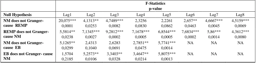
Results of Granger-causality test show that the null hypotheses which is that net migration does not Granger-cause remittances is rejected in 1, 2, 3, 6, 7, 8 year lags, at the 5 % level (see Table 6). Results show evidence of reverse causality as well.
The null hypotheses that: net migration does not Granger cause remittances is rejected for all studied lags (1–8).
Further, the null hypotheses that net migration does not Granger cause external balance are rejected for lags 1, 4,5 - at the 5 % level. The null hypotheses stating that external balance does not Granger-cause net migration are rejected for lags 2, 3, 4, 5 (at the 5 % level). Again, the results show evidence of reverse causation in both types of relations.
Table 6
Granger Causality Wald Test
F-Statistics p-value
Null Hypothesis Lag1 Lag2 Lag3 Lag4 Lag5 Lag6 Lag7 Lag8
NM does not Granger-cause REMP
20,075*** 0,0001 4,1313** 0,0253 4,7489*** 0,0082 2,3256 0,0830 2,2261 0,0862 2,657** 0,0463 4,6667*** 0,0045 4,5159*** 0,0069
REMP does not Granger-cause NM 5,5814** 0,0238 7,1345*** 0,0027 9,2812*** 0,0002 7,1678*** 0,0005 6,8544*** 0,0005 7,6834*** 0,0002 5,86*** 0,0014 4,3612*** 0,0080
NM does not Granger-cause EB
5,1265** 0,0299 2,4313 0,1040 2,6283 0,0691 2,7851** 0,0475 5,7741*** 0,0014
NA NA NA
EB does not Granger- cause NM 1,5704 0,2185 5,2573** 0,0106 3,3403** 0,0328 3,4647** 0,0214 5,8075*** 0,0013
NA NA NA
Conclusions
Growing importance of the mobility factors in contemporary economies is unquestionable (Kumpikaite & Zickute, 2012; Janotka et al., 2013, Berzinskiene et al., 2014; Kvedaraite et al., 2015).
In this paper the role that these factors play in driving migration flow has been studied and strongly highlighted. In contrast to what many believe we have demonstrated that the relations between certain mobility factors are not of one-directional character only.
Apart from this research, only a few researchers provided empirical evidence supporting causality with respect to a migration flow (Marr & Siklos, 1994; Marr & Siklos, 1999; Konya, 2000; Feridun 2004; Feridun, 2005; Morley, 2006; Feridun, 2007). The phenomenon of causality
can be demonstrated with methods such as Granger-Causality (Granger, 1969) or the Convergent Cross Mapping (Sugihara et al., 2012).
In particular this paper confirmed the impact that net migration has on remittances and external balance and vice versa. We chose the Spanish context to show that there are certain reciprocal relations between mobility factors. The results indicated that when the level of net migration increases, remittances paid also increase, and vice versa. Based upon Granger’s methodology we have demonstrated causality between migration and remittances.
In addition, as the analysis showed not only growing migration flow leads to higher remittances paid but past remittances also draw the migration flow the other way around. In other words, remittances paid encourage potential migrants. This is actually consistent with an intuitive feel. In contrast to this, positive balance of foreign trade worked the other way around.
All in all, the main finding of our study is that migration, remittances and international trade form a positive feedback loop. This sheds some light on the mobility factors mutual relations in terms of the
Heckscher-Ohlin framework. We have found that an increase of the migration flow in the analyzed period (1975–2013) could be explained partly because of the increase in remittances. What is worth emphasizing is that the growing importance of remittances will persist in the future due to a significant costs’ reduction and structural changesin the industry (i.e. technological improvements, liberal trade policies, the EU’s single market and “four freedoms” and obviously the higher number of companies in the remittance industry). Therefore, it is very likely that these mobility factors will become of relatively even higher importance in the future.
References
Adams, R. H., & Page, J. (2005). Do international migration and remittances reduce poverty in developing countries? World Development, 33, 1645–1669. http://dx.doi.org/10.1016/j.worlddev.2005.05.004
Adenutsi, D. E. (2010). Do international remittances promote human development in poor countries? Empirical evidence from Sub-Saharan Africa. The International Journal of Applied Economics and Finance, 4, 31–45. http://dx.doi.org/ 10.3923/ijaef.2010.31.45
Akkoyunlu, S., Siliverstovs, B., & Stark, O. (2007). Remittances as a harbinger of migration: An empirical macroeconomic causal link. DIW Discussion Paper.
Akkoyunlu, S., & Siliverstovs, B. (2007). The role of remittances in migration decision: Evidence from Turkish migration. DIW Discussion Paper, 691.
Akkoyunlu, S. (2009). Trade, aid, remittances and migration. KOF Working Paper, 229. http://dx.doi.org/ 10.2139/ssrn.1436356 Aldrich, J. (1995). Correlations Genuine and Spurious in Pearson and Yule. Statistical Science, 10(4), 364–376.
Arnold, F. (1992). The contribution of remittances to economic and social development, in M. Kritz, C. B. Keely and H. Zlotnik (eds) International Migration Systems: A Global Approach. Oxford: Clarendon Press.
Barajas, A., Chami, R., Fullenkamp, C., Gapen, M., & Montiel, P. (2009). Do workers’ remittances promote economic growth? IMF Working Paper, 09/153.
Berzinskiene, D., Butkus, M., & Matuzeviciute, C. (2014). Modelling of the Impact of Emigrants’ Qualification Structure on the National Economic Growth: the Case of Lithuania. Inzinerine Ekonomika-Engineering Economics, 25(3), 333– 340. http://dx.doi.org/10.5755/j01.ee.25.3.5247
Chami, R., Fullenkamp, C., & Jahjah, S. (2003). Are immigrant remittances flows a source of capital for development? IMF Working Paper, 189.Dickey, D. A., & Fuller, W. A. (1979). Distribution of the Estimators for Autoregressive Time Series with a Unit Root. Journal of American Statistical Association, 74, 13–33.
Durand, J., Parrado, E. A., & Massey, D. S. (1996). Migradollars and development: A reconsideration of the Mexican case. International Migration Review, 30, 423–444. http://dx.doi.org/10.2307/2547388
Engle, R. F., & Granger, C. W. J. (1987). Co-integration and Error Correction: Representation, Estimation and Testing. Econometrica, 55, 251–276. http://dx.doi.org/10.2307/1913236
Edwards, C., & Ureta, M. (2003). International migration, remittances, and schooling: evidence from El Salvador. Journal of Development Economics, 72(2), 429–461. http://dx.doi.org/10.1016/S0304-3878(03)00115-9
Eichler, M. (2012). Causal Inference in Time Series Analysis. In Berzuini, Carlo. Causality: statistical perspectives and applications (3. ed.). Hoboken, N.J.: Wiley, 27–352. http://dx.doi.org/10.1002/9781119945710.ch22
Faini, R., & Venturini, A., (1993). Trade, aid and migrations. Some basic policy issues. European Economic Review, 37, 435–442. http://dx.doi.org/10.1016/0014-2921(93)90032-6
Feridun, M. (2004). Does Immigration have an Impact on Economic Development and Unemployment? Empirical Evidence from Finland (1981-2001). International Journal of Applied Econometrics and Quantitative Studies, 1, 39–60. Feridun, M. (2005). Investigating the Economic Impact of Immigration on the Host Country: The Case of Norway. Prague
Economic Papers, 4, 350–362. http://dx.doi.org/10.18267/j.pep.270
Feridun, M. (2008). Immigration, income and unemployment: an application of the bounds testing approach to cointegration. Journal of Developing Areas, 41(1), 1–21. http://dx.doi.org/10.1353/jda.2008.0014
Goldin, I, & Reinert, K. (2006). Globalization for Development: Trade, Finance, Aid, Migration, and Policy. Washington and Basingstoke: World Bank and Palgrave Macmillan. http://dx.doi.org/10.1596/978-0-8213-6274-7
Granger, C. W. J. (1969), Investigating Causal Relations by Econometric Models and Cross-Spectral Methods. Econometrica, 37, 55–76. http://dx.doi.org/10.2307/1912791
Granger, C. W. J. (1980). Testing for causality: A personal viewpoint. Journal of Economic Dynamics and Control, 2, 329– 352. http://dx.doi.org/10.1016/0165-1889(80)90069-X
Granger, C. W. J. (1983a). Investigating Causal Relations by Econometric Models and Cross-Spectral Methods. Econometrica, 37, 12–15.
Granger, C. W. J. (1983b), Cointegrated variables and error-correcting models. San Diego, CA, UCSD discussion paper. Johansen, S. (1991). Estimation and Hypothesis Testing of Cointegration Vectors in Gaussian Vector Autoregressive
Models. Econometrica, 59(6), 1551–1580. http://dx.doi.org/10.2307/2938278
Findlay, R., Rolf G. H., Lindgren, H., & Lundahl, M., (eds.) (2007). Eli Heckscher, International Trade, and Economic History, The MIT Press.
Hassapis, C., Pittis, N., Prodromidis, K. (1999). Unit Roots and Granger Causality in the EMS interest rates: The German Dominance Hypothesis Revisited. Journal of International Money Finance, 18 (4), 7–73. http://dx.doi.org/10.1016/s0261-5606(98)00044-8
Johansen, S. & Juselius, K. (1990). Maximum Likelihood Estimation and Inference on Cointegration – with Applications to the Demand for Money. Oxford Bulletin of Economics and Statistics, 4, 222–234. http://dx.doi.org/10.1111/j.1468-0084.1990.mp52002003.x
Janotka, M., Gazda, V., & Horv, D. (2013). Migration Trends among Regional clusters in Slovakia. Inzinerine Ekonomika-Engineering Economics, 24(5), 437–446.
Kim, K., & Cohen, J. (2010). Determinants of International Migration Flows to and from Industrialized Countries: A Panel Data Approach beyond Gravity. International Migration Review, 4(4), 899–932. http://dx.doi.org/10.1111/j.1747-7379.2010.00830.x
Konya, L. (2000). Bivariate Causality between Immigration and Long-Term Unemployment in Australia, 1981-1998. Victoria University of Technology Working Paper, 18/00.
Kumpikaite V. & Zickute, I. (2012). Synergy of Migration Theories: Theoretical Insights. Inzinerine Ekonomika-Engineering Economics, 23(4), 387–394. http://dx.doi.org/10.5755/j01.ee.23.4.1240
Kvedaraite, N., Baksys, D., Repeckiene, A., & Glinskiene, R. (2015). Research of Experience of Emigration for Employment and Education Purposes of Students. Inzinerine Ekonomika-Engineering Economics, 26(1), 196–203. http://dx.doi.org/10.5755/j01.ee.26.2.3863
Lopez, R., & Schiff, M. (1998). Migration and the skill composition of the labour force: The impact of trade liberalisation in LDCs. Canadian Journal of Economics, 31, 318–36. http://dx.doi.org/10.2307/136326
Lundborg, P. (1991). Determinants of migration in the Nordic labour market. Scandinavian Journal of Economics, 93, 363– 375. http://dx.doi.org/10.2307/3440180
Markusen, J. R. (1983). Factor Movements and Commodity Trade as Complements. Journal of International Economics. 14(3/4), 341–356. http://dx.doi.org/10.1016/0022-1996(83)90009-0
Marr, W. L., & Siklos, P. L. (1994). The Link between Immigration and Unemployment in Canada. Journal of Policy Modeling, 16, 1-26. http://dx.doi.org/10.1016/0161-8938(94)90001-9
Marr, W. L., & Siklos, P. L. (1999). Immigrant Class and the Use of Unemployment Insurance by Recent Immigrants in Canada: Evidence from a New Data Base, 1980 to 1995. International Migration Review, 33(3), 561–593. http://dx.doi.org/10.2307/2547526
Martin, P. (1993). Trade and Migration: NAFTA and Agriculture. Institute for International Economics,Washington. Martin, P., & Taylor, J. E. (1996). The anatomy of a migration hump. In J. E. Taylor (ed) Development Strategy,
Employment and Migration: Insights from Models, 43–62, Paris: OECD.
Mitchell, J., & Pain, N. (2003). The determinants of international migration into the UK: A panel based modelling approach. NIESR Discussion Papers, 216, National Institute of Economic and Social Research.
Morley, B. (2006). Causality between Economic Growth and Immigration: An ARDL Bounds Testing Approach, Economics Letters, 90, 72–76. http://dx.doi.org/10.1016/j.econlet.2005.07.008
Mundell, R. (1957). International Trade and Factor Mobility. The American Economic Review, 47(3), 321–335.
Onley, W. (2015). Remittances and the Wages Impact of Immigration. The Journal of Human Resources, Volume 50(3), 1– 41.
Pesaran, M. H., Shin, Y., & Smith, R. J. (2001). Bounds Testing Approaches to the Analysis of Level Relationships, Journal of Applied Econometrics, 16, 289–326. http://dx.doi.org/10.1002/jae.616
Ratha, D. (2003). Workers’ remittances: An important and stable source of external development finance. Global Development Finance, 157–175, Washington: World Bank.
Russell, S., & Teitelbaum, M. (1992). Intenational Migmrtion and International Trade. World Bank Discussion Paper, 160. Saikkonen, P., & Lutkepohl, H., (2002). Testing for a unit root in a time series with a level shift at unknown time.
Econometric Theory, 18, 313–348. http://dx.doi.org/10.1017/s0266466602182053
Sargent, T. J. (1976). A Classic Macroeconometric Model for the United States. Journal of Political Economy, 84, 207–237. http://dx.doi.org/10.1086/260429
Schiff, M. (1994). How trade, aid and remittances affect international migration. Policy Research Working Paper. The World Bank International Economics Department, International Trade Division.
Sims, Ch. A. (1996). Macroeconomics and Methodology. Journal of Economic Perspectives 10(1), 105–120. http://dx.doi.org/10.1257/jep.10.1.105
Sugihara, G., May, R., Ye, H., Hsieh, C., Deyle, E., Fogarty, M., Munch, S. (2012). Detecting Causality in Complex Ecosystems. Science, 338 (6106), 496–500. Available from internet: http://www.uvm.edu/~cdanfort/csc-reading-group/sugihara-causality-science-2012.pdf
Taylor, J.E. (1999). The new economics of labour migration and the role of remittances in the migration process. International Migration, 37(1), 63–88. http://dx.doi.org/10.1111/1468-2435.00066
Tufte, E. R. (2006). The Cognitive Style of PowerPoint: Pitching Out Corrupts Within. (2nd ed.). Cheshire, Connecticut: Graphics Press, ISBN 0-9613921-5-0, p. 5 Available from internet: http://users.ha.uth.gr/tgd/pt0501/09/Tufte.pdf World Bank (2006). Global Economic Prospects. World Bank publications.Washington, DC.