Volume 2, Issue 6, December 2014
Abstract - The image de-noising naturally corrupted by noise is a classical problem in the field of signal or image processing. Additive random noise can easily be removed using simple threshold methods. De-noising of natural images corrupted by Gaussian noise and Gaussian - Gaussian Mixture using wavelet techniques are very effective because of its ability to capture the energy of a signal in few energy transform values. In this paper decompose the image using discrete wavelet and then applied PCNN (Pulse Coupled Neural Network) algorithm and threshold for mixed noise removal. The proposed method can efficiently remove a variety of mixed or single noise while preserving the image information well. It is proposed to investigate the suitability of different wavelet bases and the size of different neighborhood on the performance of image de-noising algorithms in terms of PSNR. The experimental results demonstrate its better performance compared with some existing methods.
Keywords - Image, De-noising, Wavelet, Transform, PCNN, mixed noise.
I. INTRODUCTION
Over the past decade, wavelet transforms have received a lot of attention from researchers in many different areas. Both discrete and continuous wavelet transforms have shown great promise in such diverse fields as image compression, image de-noising, signal processing, computer graphics, and pattern recognition to name only a few. In de-noising, single orthogonal wavelets with a single-mother wavelet function have played an important role. De-noising of natural images corrupted by Gaussian noise and Gaussian - Gaussian Mixture using wavelet techniques is very effective because of its ability to capture the energy of a signal in few energy transform values. Crudely, it states that the wavelet transform yields a large number of small coefficients and a small number of large coefficients.
Here the classical Gaussian and Gaussian-Gaussian mixed noise removal problem in this paper, where the noise in the images can be modeled by
g = f + n ………… (1)
where g, f, n are the observed image, clean image, and noise, respectively. In the overwhelming majority of literature results, the noise n is supposed to be a Gaussian distribution.
For Gaussian noise removal, variational method becomes one of the most popular and powerful tools for image restoration since the total variation (TV) was proposed in [1]. The TVL2 or the so-called ROF model [1] is a classical and well-known model to remove Gaussian noise. However, the results obtained with TV could be over-smoothed and the image details such as textures could be removed together with noise. In order to better preserve the image textures, the nonlocal denoising method was integrated with variational method and the nonlocal TV models in [2], [3]. The nonlocal TV greatly improves the denoising results, but the nonlocal weights in these models may be difficult to determine. Another Gaussian noise removal approach is to use wavelet shrinkage. The high frequency coefficients are suppressed with some given rules such as shrinking. Sparse representation and dictionary learning is also a highly effective image denoising technique. In [4], [5], the authors proposed a novel method to remove additive white Gaussian noise using PCNN for learning the dictionary from the noisy image with gray scale images.
II. DISCRETEWAVELETTRANSFORM
The Discrete Wavelet Transform (DWT) of image signals produces a non- redundant image representation, which provides better spatial and spectral localization of image formation, compared with other multi scale representations such as Gaussian and Laplacian pyramid. Recently, Discrete Wavelet Transform has attracted more and more interest in image de-noising. The DWT can be interpreted as signal decomposition in a set of
Mixed Noise Reduction based on improved
PCNN Algorithm
Shajun Nisha, Kother Mohideen,
Research Scholar, Department of Computer Science, Bharathiar University, Coimbatore
Volume 2, Issue 6, December 2014
independent, spatially oriented frequency channels. The signal S is passed through two complementary filters and emerges as two signals, approximation and Details. This is called decomposition or analysis. The components can be assembled back into the original signal without loss of information. This process is called reconstruction or synthesis. The mathematical manipulation, which implies analysis and synthesis, is called discrete wavelet transform and inverse discrete wavelet transform. An image can be decomposed into a sequence of different spatial resolution images using DWT. In case of a 2D image, an N level decomposition can be performed resulting in 3N+1different frequency bands namely, LL, LH, HL and HH as shown in figure 1. These are also known by other names, the sub-bands may be respectively called a1 or the first average image, h1 called horizontal fluctuation, v1 called vertical fluctuation and d1 called the first diagonal fluctuation. The sub-image a1 is formed by computing the trends along rows of the image followed by computing trends along its columns. In the same manner, fluctuations are also created by computing trends along rows followed by trends along columns. The next level of wavelet transform is applied to the low frequency sub band image LL only. The Gaussian noise will nearly be averaged out in low frequency wavelet coefficients. Therefore, only the wavelet coefficients in the high frequency levels need to be thresholded.
Fig 1. 2D-DWT with 3-Level decomposition
III. WAVELETBASEDIMAGEDE-NOISING
All digital images contain some degree of noise. Image denoising algorithm attempts to remove this noise from the image. Ideally, the resulting de-noised image will not contain any noise or added artifacts. De-noising of natural images corrupted by Gaussian noise using wavelet techniques is very effective because of its ability to capture the energy of a signal in few energy transform values. The methodology of the discrete wavelet transform based image de-noising has the following three steps as shown in figure 2. 1. Transform the noisy image into orthogonal domain by discrete 2D wavelet transform. 2. Apply PCNN algorithm 3. Apply hard or soft thresholding the noisy detail coefficients of the wavelet transform 4. Perform inverse discrete wavelet transform to obtain the de-noised image.
Here, the threshold plays an important role in the denoising process. Finding an optimum threshold is a tedious process. A small threshold value will retain the noisy coefficients whereas a large threshold value leads to the loss of coefficients that carry image signal details. Normally, hard thresholding and soft thresholding techniques are used for such de-noising process. Hard thresholding is a keep or kill rule whereas soft thresholding shrinks the coefficients above the threshold in absolute value. It is a shrink or kill rule.
Fig 2. Diagram of wavelet based image De-noising
PCNN Method
In this method, Denoising is done by soft-thresholding the wavelet co-efficient. PCNN is used to determine the heavy tailed co-efficient in the wavelet domain.
PCNN model is a single layer two-dimensional array of laterally linked neurons and all neurons are identical. Each neuron is corresponding to an image pixel, and the whole neurons are laterally linked as the PCNN model.
Original Image
Add mixed noise
Log Transform
DWT Applied PCNN Method
Inverse DWT
Exponential Transform
Reconstructe d Image
LL
3LH
3HL
3HH
3HL
2LH
2HH
2LH
1Volume 2, Issue 6, December 2014
Generally, every neuron is made up of dendritic tree, linking modulation, and pulse generator, which can describe as follows: ij kl ijkl F ij F
ij
n
F
n
V
M
Y
n
I
F
[
]
exp(
)
[
1
]
(
1
)
(1))
1
(
]
1
[
)
exp(
]
[
n
L
n
V
W
Y
n
L
ij
L ij L ijkl kl (2)])
[
1
](
[
]
[
n
F
n
L
n
U
ij
ij
ij (3)
]
[
n
Yij
otherwise
n
T
n
U
,
0
]
[
]
[
-£
1
ij
ij(4)
]
[
]
1
[
)
exp(
]
[
n
T
n
V
Y
n
T
ij
T ij
T ij (5)As the top formulas, Iij, Fij, Lij, Uij, Yij, Tij mean separately neurons’ outside stimulating input, feed-in input, linking
input, inside activity, firing output, dynamic threshold. M and W are linking weight matrix (usually, M = W), VF, VL,
VTmean separately inherent electricity in Fij, Lij and Tij,,αF, αL, αT mean separately attenuation time constants in Fij,
Lij, Tij, n is a loop constant, and Yij is a binary output.
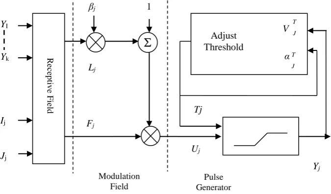
As shown in figure 1, the neuron receives input signals from other neurons and from external sources through the receptive field. In general, the signals from other neurons are pulses; the signals from external sources are analog timing-varying signals constants or pulses. After inputting the receptive field, input signals are divided into two channels. One channel is feed-in input (Fij); the other is linking input (Lij). In general, the feeding connection has a
slower characteristic response time constant that that of the linking connection. In modulation field, see Fig.1 and Equ. (3), at first, the linking input is added a constant positive bias. Then it is multiplied by the feed-in input. The bias is taken to be unity, β is the linking strength. The total inside activity Uij is the result of modulation. Because
the feed-in input has a slower characteristic response time constant that that of the linking input, Uij is like a spike
like signal riding on an approximate constant. The pulse generator consists of a threshold adjuster, a threshold Tij
changes with the variation of the neuron’s output pulse. When the neuron emits a pulse, it feeds back to increase the threshold. When Tijarises more than Uij, the pulse creator closes and stop emitting pulses. Then threshold value
drops. When threshold Tij drops less than Uij, the pulse creator opens again and emits pulses, namely fires. If the
neuron only emits a pulse when it fires, the threshold discriminator and the pulse former can be replaced by a step function. This method is shown in Fig.1. Meanwhile, Equ.(4) shows the neuron’s output under signal output pulse
condition and Yij is the output. Connecting the neurons on another, then a PCNN model appears.
Fig. 3 The model neuron of PCNN YI Yk Modulation Field Adjust Threshold Pulse Generator Re ce p ti v e F ield Ij Jj
βj 1
Lj
Fj
Uj
Tj
V T J
α T J
Volume 2, Issue 6, December 2014
A. Probability Density Functions of Mixed Noise
Here additive mixed noise removal via energy minimization method. For real images, the probability density function (PDF) is often not a single standardized distribution such as Gaussian. Thus its MLE is often difficult to solve.
Here we consider the case that the noise is sampled from several different distributions. This mixed noise in images is more difficult to remove than the standardized Gaussian noise. And also described the framework for restoring images corrupted by mixed noise.
Suppose the mixed noise n ∈ RS1S2 is constituted by M different groups nl , l = 1, 2, . . . , M, each sl is some
realizations of a random variable Sl with PDF pl(x), and the ratio of each s1 is rl. Here rl satisfies_M l=1 rl = 1. Similarly, s can also be regarded as some realizations of a random variable N whose PDF is p(x). With these assumptions, one can get the PDF of mixed noise
p(x) =M_l=1rl pl(x) ………… (2)
B. Threshold Methods
The following are the methods of threshold selection for image de-noising based on wavelet transform
Method 1: Visushrink
Threshold T can be calculated using the formulae,
T= σ√2logn2 ………… (3)
This method performs well under a number of applications because wavelet transform has the compaction property of having only a small number of large coefficients. All the rest wavelet coefficients are very small. This algorithm offers the advantages of smoothness and adaptation. However, it exhibits visual artifacts.
Method 2: Neighshrink
Let d(i,j) denote the wavelet coefficients of interest and B(i,j) is a neighborhood window around d(i,j). Also let S2=Σd2(i,j) over the window B(i,j). Then the wavelet coefficient to be thresholded is shrinked according to the formulae, d(i,j)= d(i,j)* B(i,j) ….(4) where the shrinkage factor can be defined as B(i,j) = ( 1- T2/ S2(i,j))+, and the sign + at the end of the formulae means to keep the positive value while set it to zero when it is negative.
Method 3: Modineighshrink
During experimentation, it was seen that when the noise content was high, the reconstructed image using Neighshrink contained mat like aberrations. These aberrations could be removed by wiener filtering the reconstructed image at the last stage of IDWT. The cost of additional filtering was slight reduction in sharpness of the reconstructed image. However, there was a slight improvement in the PSNR of the reconstructed image using wiener filtering. The de-noised image using Neighshrink sometimes unacceptably blurred and lost some details. So that it has been processed by K-VSD algorithm and then threshold for the shrinkage the coefficients. In earlier methods the suppression of too many detail wavelet coefficients. This problem will be avoided by reducing the value of threshold itself. So, the shrinkage factor is given by
B(i,j) = ( 1- (3/4)*T2/ S2(i,j))+ ………… (4)
Method 4: SureShrink
SureShrink is a thresholding technique in which adaptive threshold is applied to sub band, but a separate threshold is computed for each detail sub band based upon SURE (Stein.s Unbiased Estimator for Risk), a method for estimating the loss in an unbiased fashion. The optimal λ and L of every sub band should be data-driven and should minimize the Mean Squared Error (MSE) or risk of the corresponding sub band. Fortunately, Stein has stated that the MSE can be estimated unbiased from the observed data. Neighshrink can be improved by determining an optimal threshold and neighbouring window size for every wavelet sub band using the Stein’s Unbiased Risk Estimate (SURE). For ease of notation, the Ns noisy wavelet coefficients from sub band s can be arranged into the
1-D vector. Similarly, the
N
s unknown noiseless coefficients from subband ‘s’ is combined with thecorresponding 1-D vector. Stein shows that, for almost any fixed estimator
sbased on the dataw
s, the expectedloss (i.e risk)
2
2
s s
E
can be estimated unbiasedly. Usually, the noise standard deviation is set at 1, andVolume 2, Issue 6, December 2014
2
(
)
222
.
(
)
2 s s s
s
s
N
E
g
w
g
w
E
(5,8)
n
n n s
s N n n
s
g
w
g
g
w
w
g
(
)
{
}
s,
.
/
1
(5,9)IV. EVALUATIONCRITERIA
The above said methods are evaluated using the quality measure Peak Signal to Noise ratio which is calculated using the formulae,
PSNR= 10log 10 (255) 2/MSE (db) … (5)
Where MSE is the mean squared error between the original image and the econstructed de-noised image. It is used to evaluate the different de-noising scheme like Wiener filter, Visushrink, Neighshrink, Modified Neighshrink and Sureshrink.
V. EXPERIMENTS
Quantitatively assessing the performance in practical application is complicated issue because the ideal image is normally unknown at the receiver end. So this paper uses the following method for experiments. One original image is applied with Gaussian noise and Gaussian – Gaussian mixed noise with different variance. The methods proposed for implementing image de-noising using wavelet transform take the following form in general. The image is transformed into the orthogonal domain by taking the wavelet transform.
The detail wavelet coefficients are modified according to the shrinkage algorithm. Finally, inverse wavelet is taken to reconstruct the de-noised image. In this paper, different wavelet bases are used in all methods. For taking the wavelet transform of the image, readily available MATLAB routines are taken. In each sub-band, individual pixels of the image are shrinked based on the threshold selection. A de-noised wavelet transform is created by shrinking pixels. The inverse wavelet transform is the de-noised image.
VI. RESULTSANDDISCUSSIONS
For the above mentioned three methods, image de-noising is performed using wavelets from the second level to fourth level decomposition and the results are shown in figure (3) and table if formulated for second level decomposition for different noise variance as follows. It was found that three level decomposition and fourth level decomposition gave optimum results. However, third and fourth level decomposition resulted in more blurring. The higher level of blurred by PCNN algorithm. The experiments were done using a window size of 3X3, 5X5 and 7X7. So here 7X7 neighborhood window size results are shown.
Window Size 7 x 7
Variance 0.02 0.04 0.06 0.08
Noisy Image 16.8464 14.1031 12.6412 11.6592
Wiener 26.6335 24.8262 23.732 22.9097
Wavelet
Type Threshold Type
Harr Visushrink 22.2856 19.8075 18.3325 17.4044
Neighshrink 24.5573 23.2544 22.2874 21.5715
ModiNeighshrink 25.9578 24.9888 24.0934 23.3887
Sureshrink 26.9704 26.0222 25.1312 24.5012
db 16 Visushrink 22.6147 19.9770 18.5080 17.5385
Neighshrink 23.3666 22.3595 21.6294 21.0237
Volume 2, Issue 6, December 2014
Sureshrink 25.4412 24.9421 24.1121 24.5995
Sym 8 Visushrink 22.6058 19.984 18.454 17.4988
Neighshrink 23.4157 22.4825 21.6285 21.0469
ModiNeighshrink 24.3611 23.8334 23.1595 22.6622
Sureshrink 25.3895 24.8725 24.2058 23.7335
Coif 5 Visushrink 22.6153 19.917 18.486 17.4952
Neighshrink 26.0615 24.2785 23.1234 22.2693
ModiNeighshrink 27.2978 25.9815 24.9992 24.1564
Sureshrink 29.3458 28.4555 27.3464 26.5781
For Different Threshold Methods with Wavelet Domain Image Window Size 7X7 for mixed noise
VII. CONCLUSION
In this paper, the image de-noising using discrete wavelet transform is analyzed with PCNN algorithm. The experiments were conducted to study the suitability of different wavelet bases and also different window sizes. Among all discrete wavelet bases, coiflet performs well in image de-noising. Experimental results also show that Sureshrink gives better result than modified Neighshrink, Weiner filter and Visushrink for mixed noise.
REFERENCES
[1] L. I. Rudin, S. Osher, and E. Fatemi, “Nonlinear total variation based noise removal algorithms,” Phys. D, Nonlinear Phenomena, vol. 60, nos. 1–4, pp. 259–268, Nov. 1992.
[2] G. Gilboa and S. Osher, “Nonlocal linear image regularization and supervised segmentation,” Multiscale Model. Simul. vol. 6, no. 2, pp. 595–630, Jan. 2007.
[3] G. Gilboa and S. Osher, “Nonlocal operators with applications to image processing,” SIAM Multiscale Model. Simul. vol. 7, no. 3, pp. 1005–1028, 2008.
[4] M. Elad and M. Aharon, “Image denoising via learned dictionaries and sparse representation,” in Proc. IEEE Comput. Vis. Pattern Recognit., Jun. 2006, pp. 895–900.
[5] M. Elad and M. Aharon, “Image denoising via sparse and redundant representations over learned dictionaries,” IEEE Trans. Image Process., vol. 15, no. 12, pp. 3736–3745, Dec. 2006.
[6] A Weighted Dictionary Learning Model for Denoising Images Corrupted by Mixed Noise “Jun Liu, Xue-Cheng Tai, Haiyang Huang, and Zhongdan Huan, Ieee Transactions On Image Processing, Vol. 22, No. 3, March 2013
[7] D. L. Donoho, “Denoising by soft-thresholding,” IEEE Transactions on Information Theory, vol. 41, pp.613-627, 1995.
[8] Bui and G. Y. Chen, “Translation invariant de-noising using multiwavelets,” IEEE Transactions on Signal Processing, vol.46, no.12, pp.3414-3420, 1998.
[9] L. Sendur and I. W. Selesnick, “Bi-variate Shrinkage with Local Variance Estimation,” IEEE Signal Processing Letters, Vol. 9, No. 12, pp. 438-441,2002.
[10]G. Y. Chen and T. D. Bui, “Multi-wavelet De-noising using Neighboring Coefficients,” IEEE Signal Processing Letters, vol.10, no.7, pp.211-214, 2003.
Original Image Noise Image Visushrink Denoised image
using Neighshrink
Volume 2, Issue 6, December 2014
[11]S.Kother Mohideen, Dr. S. Arumuga Perumal, and Dr. M.Mohamed Sathik, “Image De-noising using Discrete Wavelet transform,” IJCSNS International Journal of Computer Science and Network Security, VOL.8 No.1, January 2008.
[12]Saraswathi Janaki samusarma, Mary Brinda,” Denoising of Mixed Noise in Ultrasound Images,” IJCSI International Journal of Computer Science Issues, VOL 8,Issue 4, No 1, July 2011.
[13]S.Shajun Nisha, Dr. S. Kother Mohideen, “A Novel Approach for Image Mixed Noise Reduction Using Wavelet Method,” IJARCSSE International Journal of Advanced Research in Computer Science and Software Engineering, VOL.3, Issue 11,November 2013.
AUTHOR BIOGRAPHY
Prof.S.Shajun Nisha Research Scholar in Computer Science, Bharathiar University, Coimbatore. She has completed M.Phil.(Computer Science) and M.Tech (Computer and Information Technology) in Manonmaniam Sundaranar University, Tirunelveli. She has involved in various academic activities. She has attended so many national and international seminars, conferences and presented numerous research papers. She is a member of ISTE and IEANG and her specialization is Image Mining.