S H O R T R E P O R T
Open Access
Clarifications regarding the use of model-fitting
methods of kinetic analysis for determining the
activation energy from a single non-isothermal
curve
Pedro E Sánchez-Jiménez
*, Luis A Pérez-Maqueda, Antonio Perejón and José M Criado
Abstract
Background:This paper provides some clarifications regarding the use of model-fitting methods of kinetic analysis for estimating the activation energy of a process, in response to some results recently published in Chemistry Central journal.
Findings:The model fitting methods of Arrhenius and Savata are used to determine the activation energy of a single simulated curve. It is shown that most kinetic models correctly fit the data, each providing a different value for the activation energy. Therefore it is not really possible to determine the correct activation energy from a single non-isothermal curve. On the other hand, when a set of curves are recorded under different heating schedules are used, the correct kinetic parameters can be clearly discerned.
Conclusions:Here, it is shown that the activation energy and the kinetic model cannot be unambiguously determined from a single experimental curve recorded under non isothermal conditions. Thus, the use of a set of curves recorded under different heating schedules is mandatory if model-fitting methods are employed.
Findings
In a paper recently published in the Chemistry Central Journal, a kinetic study of the thermal decomposition of both aged and non-aged commercial cellulosic paper was presented, and the apparent activation energy (Ea) of the degradation reaction was determined for each case [1]. According to the authors, the Ea of the process is related to the breakdown of cellulose chains and, since the apparent activation energy of the process is found to decrease with the aging time of the cellulose paper, it is proposed that such evolution could be used to construct archaeometric curves. Three different model-fitting methods were used to determine the activation energy: the differential Arrhenius method, the integral Savata method and the Wyden-Widmann method. Also, the authors speculate with the possibility that the kinetic method selected influences the obtained Ea. Actually,
when using the Wyden-Widmann method, it is observed that only a limited number of data points around the DTG peak should be employed or else the Ea obtained would not fit that obtained by the other kin-etic methods. Finally, it is concluded that a first order model is the most suitable for describing the cellulose decomposition reaction. However, recent works have reached to different conclusions, finding a chain scis-sion model to be far more appropriate [2]. Such dis-crepancy is due to some fundamental misconceptions in the manner the kinetic methods are employed in Marini’s work. Firstly, the activation energy for every sample studied was obtained by means of applying a model-fitting method to experimental data proceeding from a single non-isothermal run. Secondly, only the fit to two kinetic models, F1 and A2, were explored in the analysis. Basically, model-fitting methods of kinetic analysis consist of fitting the experimental data to a series of theoretical kinetic models, which are algebraic functions that reflect the relationship between * Correspondence:[email protected]
Instituto de Ciencia de Materiales de Sevilla, C.S.I.C.-Universidad de Sevilla, C. Américo Vespucio nº49, Sevilla 41092, Spain
© 2013 Sánchez-Jiménez et al.; licensee Chemistry Central Ltd. This is an Open Access article distributed under the terms of the Creative Commons Attribution License (http://creativecommons.org/licenses/by/2.0), which permits unrestricted use, distribution, and reproduction in any medium, provided the original work is properly cited.
reaction rate and degree of conversion and can be related to the reaction mechanism. The model provid-ing the best linear fit is usually regarded as the cor-rect one, and the activation energy is deduced from the slope of the fit. Unfortunately, it has been long established that the activation energy cannot be reli-ably determined from a single non isothermal curve because the experimental data almost always provides a reasonable fit regardless the kinetic model selected [3-5]. Despite that significant flaw, such inappropriate practice is still nevertheless widely used. As a result,
it is common that nth order models are incorrectly
selected because they are often tested as the first op-tion for simplicity and a good fit is usually obtained. Here, we attempt to throw some light on the use of model-fitting methods and clarify such still wide-spread misuses.
Results and Discussion
Figure 1 includes a simulated α-T curve, constructed
as-suming a heating rate of 10 K min-1 and the following
kinetic parameters: Ea=150 kJ/mol, A=1010 s-1and a F1
(first order) kinetic model. The model-fitting methods of
Arrhenius and Savata, those used in Marini’s work
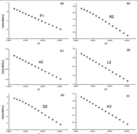
[1], were selected to determine the activation energy of the simulated curve. Thus, from the simulated data, the left hand of Eqs (1) and (2), corresponding to the Arrhenius and Savata methods respectively and shown in the Methods section, are plotted vs. the inverse of the temperature considering several of the most usual models in the literature. The f(α) and g(α) functions are listed in Table 1. The resulting activa-tion energies, as obtained from the slope of the plots, and the regression coefficients showing the quality of the fits are included for the Arrhenius and Savata
Figure 1Kinetic curve simulated according the following kinetic parameters: Ea=150 kJ/mol, A=1010s-1, and a F1 kinetic model.
Table 1 f(α) and g(α) kinetic functions corresponding to the most widely employed kinetic models
Mechanism Symbol f(α) f(α)
Phase boundary controlled reaction (contracting area) R2 2(1−α)1/2 2[1−(1−α)1/2]
Phase boundary controlled reaction (contracting volume) R3 3(1−α)2/3 3[1−(1−α)2/3]
First order kinetics or Random nucleation followed by an instantaneous growth of nuclei. (Avrami-Erofeev eqn.n=1)
F1 (1−α) −ln(1−α)
Random nucleation and growth of nuclei through different nucleation and nucleus growth models. (Avrami-Erofeev eqn≠1.)
An n(1−α) [−ln(1−α)]1−1/n [
−ln(1−α)]1−1/n
Two-dimensional diffusion D2 1/[−ln(1−α)] (1−α)ln(1−α) +α
Three-dimensional diffusion (Jander equation) D3 3 1ðαÞ2=3
2 1½ð1αÞ1=3 [1−(1−α)
1/3
]2
Three-dimensional diffusion (Ginstling-Brounshtein equation) D4 3
2 1ðαÞ1=3 1
½ (1−2α/3)−(1−α)2/3
Random Scission L=2 [10] L2 2(α1/2−α) −2 ln(α1/2−1)
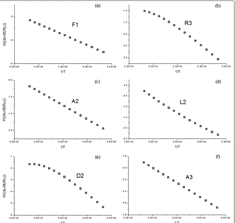
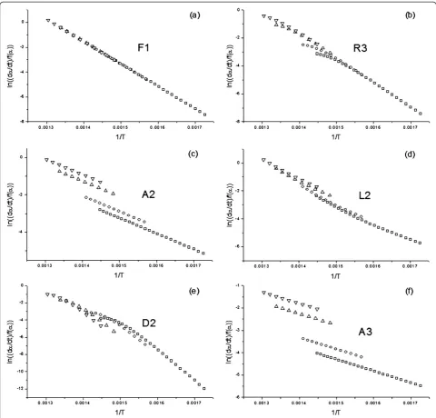
methods in Tables 2 and 3, respectively. Additionally, Figures 2 and 3 shows a selection of the plots resul-ting from the fitresul-ting of the data to the different kinetic models, so that the quality of the fit is clearly
illustrated. Thus, when the simulated curve is
analyzed by the Arrhenius method, six out of nine models deliver excellent fits to the data, with regres-sion coefficients over 0.99. Therefore, it is not really possible to effectively discern the correct model with this procedure. Moreover, as it can be observed by the values in Table 2, the activation energy obtained from the analysis is highly dependent on the kinetic model assumed, with only the fit to F1 yielding the correct value. Consequently, without further evidence regarding the correct kinetic model, the activation en-ergy cannot be established. The results are even more
problematic when the Savata model is employed (Table 3 and Figure 3). Using such method the fit to all models tested are excellent and no clear candidate can be appropriately selected.
Consequently, neither the model nor the activation energy can be deduced from the use of a model-fitting method of kinetic analysis and a single non-isothermal curve. Note that this conclusion is reached after analy-zing simulated, error-free data. When using experimen-tal data it is probable that even a higher percentage of the tested models will adequately fit such data. Thus, in order to unambiguously determine the kinetic parameters by a model-fitting procedure, a set of experimental curves, each recorded under different heating schedules, must be employed [3,6]. Then, a set of four curves simulated assuming the aforemen-tioned kinetic parameters and heating rates of 1, 2,
10 and 20 K min-1 were analyzed simultaneously
using the Arrhenius method. The resulting plots are shown in Figure 4. As it can be clearly noticed, only when the tested model is the right one, F1 in this case, are the plots positioned along a straight line. Therefore, using a set of curves recorded under different heating schedules, it is possible to unambiguously determine the kinetic model and, consequently, the activation energy.
As a final note, it should be considered that these methods are proposed for single step reactions, which can be described by a single kinetic triplet. When more than one process is taking place, each of them is expected to be defined by a different triplet. The
thermogravimetric curves included in Marini’s work
explicitly show a complex, multistep process and, therefore, such model-fitting methods cannot be employed. It is then recommended to resort to iso-conversional methods or attempt the deconvolution of the contributing steps in order to study them independently [3,7-9].
The uncertain results provided by the
Wyden-Widmann method in Marini’s work can be likewise
explained. It is still a model-fitting method since it
assumes the process is driven by an nth order kinetic
model. As it has been reported elsewhere, an nth
order model is described by a mathematical function that cannot replicate the initial induction period typ-ical of the function describing a chain scission model [10]. Thus, being the wrong model to describe the reaction, it is understandable that the required lin-earity is not achieved along the entire temperature range, as described in the paper. Had the experimen-tal data been fitted to the right model, such depend-ence of the activation energy on the number of data points considered would most probably have not been found.
Table 2 Activation energies and regression coefficients obtained from fitting the data from the simulated curve in Figure 1 to some of the most common ideal models employed in the literature, according to the Arrhenius method
Model Corr. Factor r Ea (kJ mol-1)
F1 1.000 150
R2 0.980 122
R3 0.992 131
A1.5 0.999 96
A2 0.999 69
A3 0.999 43
D2 0.982 257
D3 0.989 266
L2 0.993 100
The activation energy is determined form the slope of the plots in Figure2.
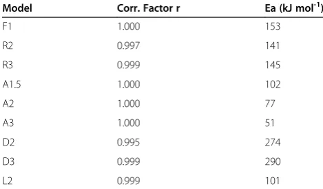
Table 3 Activation energies and regression coefficients obtained from fitting the data from the simulated curve in Figure 1 to some of the most common ideal models employed in the literature, according to the Savata method
Model Corr. Factor r Ea (kJ mol-1)
F1 1.000 153
R2 0.997 141
R3 0.999 145
A1.5 1.000 102
A2 1.000 77
A3 1.000 51
D2 0.995 274
D3 0.999 290
L2 0.999 101
The activation energy is determined form the slope of the plots in Figure3.
Sánchez-Jiménezet al. Chemistry Central Journal2013,7:25 Page 3 of 7
Conclusions
It has been shown that the activation energy cannot be reliably determined by applying model-fitting methods of kinetic analysis to data obtained under non isothermal experimental conditions. Thus, the use of a set of curves recorded under different heating schedules is necessary, as recently recom-mended by the ICTAC Kinetics Committee [3]. It is also important to consider the nature of the reac-tion under study since only one step processes can
be analyzed by this methodology. More complex or multiple step reactions require the use of isocon-versional methods or the deconvolution of the indi-vidual steps.
Methods
The simulated curves were constructed using a
Runge–Kutta 4th order numerical integration method
by means of the Mathcad software (Mathsoft, Needham, MA, USA).
Figure 2Plots obtained from fitting the data from the simulated curve (Ea=150 kJ/mol, A=1010s-1, and a F1 kinetic model) in Figure 1
The Arrhenius method is based in the following equation:
ln d∝=dt fð Þ∝
¼lnA E
RT ð1Þ
where dα/dt is the reaction rate, f(α) is the kinetic model, A the preexponential factor, E the activation energy and T the temperature in Kelvin. The Savata method relies in the following equation, which is
obtained after integrating the expression above and reordenating terms:
log g½ ð Þ∝ ¼ 0:4567 E
RT2:315þlog AE
R ð2Þ
where g(α) is the integral form of the kinetic model.
For determining the activation energy, the left-hand side of Eqs (1) and (2) are plotted against the inverse of the temperature. The value of the activation energy is then deducted from the slope of such plot.
Figure 3Plots obtained from fitting the data from the simulated curve (Ea=150 kJ/mol, A=1010s-1, and a F1 kinetic model) in Figure 1
to some of the most usual kinetic models by means of Savata model-fitting procedure.
Sánchez-Jiménezet al. Chemistry Central Journal2013,7:25 Page 5 of 7
Competing interests
The authors declare that they have no competing interests.
Authors’contribution
PSJ and AP performed the kinetic analysis of the simulated curves presented in this paper. The draft was prepared by PSJ and edited into final form by LPM. JC coordinated the study. All authors read and approved the final manuscript.
Acknowledgements
Financial support from project CTQ2011-27626 (Spanish Ministerio de Economía y Competitividad) and FEDER funds is acknowledged. Additionally, one of the authors (PESJ) is supported by a JAE-Doc grant (CSIC-FSE). We acknowledge support of the publication fee by the CSIC Open Access
Publication Support Initiative through its Unit of Information Resources for Research (URICI).
Received: 21 December 2012 Accepted: 25 January 2013 Published: 5 February 2013
References
1. Marini F, Tomassetti M, Vecchio S:Detailed kinetic and chemometric study of the cellulose thermal breakdown in artificially aged and non aged commercial paper. Different methods for computing activation energy as an assessment model in archaeometric applications.Chem Cent J 2012,6(Suppl 2):S7.
2. Sanchez-Jimenez PE, Perez-Maqueda LA, Perejon A, Pascual-Cosp J, Benitez-Guerrero M, Criado JM:An improved model for the kinetic description of the thermal degradation of cellulose.Cellulose2011,18(6):1487–1498.
Figure 4Plots obtained from fitting a set of simulated curves (Ea=150 kJ/mol, A=1010s-1, and a F1 kinetic model) assuming heating
3. Vyazovkin S, Burnham AK, Criado JM, Perez-Maqueda LA, Popescu C, Sbirrazzuoli N:ICTAC Kinetics Committee recommendations for performing kinetic computations on thermal analysis data.Thermochim Acta2011,520(1–2):1–19.
4. Brown ME:Steps in a minefield - Some kinetic aspects of thermal analysis.J Therm Anal1997,49(1):17–32.
5. Criado JM, Ortega A:Remarks on the discrimination of the kinetics of solid-state reactions from a single non-isothermal trace.J Therm Anal 1984,29(6):1225–1236.
6. Sanchez-Jimenez PE, Perez-Maqueda LA, Perejon A, Criado JM:Combined kinetic analysis of thermal degradation of polymeric materials under any thermal pathway.Polym Degrad Stab2009,94(11):2079–2085.
7. Perejon A, Sanchez-Jimenez PE, Criado JM, PerezMaqueda LA:Kinetic Analysis of Complex Solid State Reactions. A New Deconvolution Procedure.J Phys Chem B2011,115:1780–1791.
8. Vyazovkin S:Model-free kinetics - Staying free of multiplying entities without necessity.J Therm Anal Calorim2006,83(1):45–51.
9. Sanchez-Jimenez PE, Perejon A, Criado JM, Dianez MJ, Perez-Maqueda LA: Kinetic model for thermal dehydrochlorination of poly(vinyl chloride). Polymer2010,51(17):3998–4007.
10. Sanchez-Jimenez PE, Perez-Maqueda LA, Perejon A, Criado JM:A new model for the kinetic analysis of thermal degradation of polymers driven by random scission.Polym Degrad Stab2010,95(5):733–739.
doi:10.1186/1752-153X-7-25
Cite this article as:Sánchez-Jiménezet al.:Clarifications regarding the use of model-fitting methods of kinetic analysis for determining the activation energy from a single non-isothermal curve.Chemistry Central Journal20137:25.
Open access provides opportunities to our colleagues in other parts of the globe, by allowing
anyone to view the content free of charge.
Publish with
Chemistry
Central and every
scientist can read your work free of charge
W. Jeffery Hurst, The Hershey Company.
available free of charge to the entire scientific community peer reviewed and published immediately upon acceptance cited in PubMed and archived on PubMed Central yours you keep the copyright
Submit your manuscript here:
http://www.chemistrycentral.com/manuscript/
Sánchez-Jiménezet al. Chemistry Central Journal2013,7:25 Page 7 of 7