Department of Mathematics
Ph.D. Programme in Mathematics
XXIX cycle
Optimal Codes and
Entropy Extractors
Alessio Meneghetti
University of Trento
Ph.D. Programme in Mathematics Doctoral thesis in Mathematics
OPTIMAL CODES AND
ENTROPY EXTRACTORS
Alessio Meneghetti
Advisor: Prof. Massimiliano Sala
Head of the School: Prof. Valter Moretti Academic years: 2013–2016
Acknowledgements
I thank Dr. Eleonora Guerrini, whose Ph.D. Thesis inspired me and
whose help was crucial for my research on Coding Theory.
I also thank Dr. Alessandro Tomasi, without whose cooperation this
work on Entropy Extraction would not have come in the present form.
Finally, I sincerely thank Prof. Massimiliano Sala for his guidance
and useful advice over the past few years.
This research was funded by the Autonomous Province of Trento,
Call “Grandi Progetti 2012”, project On silicon quantum optics for quantum computing and secure communications - SiQuro.
Contents
List of Figures . . . v
List of Tables . . . vii
Introduction 1 I Codes and Random Number Generation 7 1 Introduction to Coding Theory 9 1.1 Definition of systematic codes . . . 16
1.2 Puncturing, shortening and extending . . . 18
2 Bounds on code parameters 27 2.1 Sphere packing bound . . . 29
2.2 Gilbert bound. . . 29
2.3 Varshamov bound . . . 30
2.4 Singleton bound . . . 31
2.5 Griesmer bound. . . 33
2.6 Plotkin bound. . . 34
2.7 Johnson bounds. . . 36
2.8 Elias bound . . . 40
2.9 Zinoviev-Litsyn-Laihonen bound . . . 42
2.10 Bellini-Guerrini-Sala bounds. . . 43
3.1 Hadamard matrices. . . 50
3.2 Hadamard codes . . . 53
4 Introduction to Random Number Generation 59 4.1 Entropy extractors . . . 62
4.1.1 Von Neumann procedure . . . 63
4.1.2 Binary linear extractors . . . 63
II Main Results 67 5 On optimal systematic codes 69 5.1 The Griesmer bound and systematic codes. . . 72
5.1.1 The cased≤2q . . . 73
5.1.2 The caseqk−1 |d . . . . 73
5.1.3 The caseq = 2,d= 2r−2s . . . 75
5.2 Versions of the Griesmer bound holding for nonlinear codes. . . 81
5.2.1 Bound A . . . 81
5.2.2 Bound B . . . 83
5.2.3 Bound C . . . 84
5.3 Classification of optimal binary codes with 4 codewords 85 5.4 On the structure of optimal binary codes with 8 code-words . . . 87
5.5 A family of optimal systematic codes . . . 90
6 Entropy extractors and Codes 95 6.1 A generalisation of the Von Neumann procedure . . . 96
6.2 New bounds for linear extractors . . . 103
6.2.1 Total variation distance and the Walsh-Hadamard transform . . . 104
6.2.2 W-H bound on binary generator matrices as
ex-tractors . . . 108
6.2.3 Total variation distance and the Fourier transform110 6.2.4 Fourier bound on entropy extractors . . . 119
6.2.5 Non-linear codes . . . 122
7 Other results 125 7.1 An improvement of known bounds on code parameters 126 7.2 The binary M¨obius transform . . . 128
7.3 A probabilistic algorithm for the weight distribution . 134 A Tables of bounds 143 A.1 Bounds for codes in F2 . . . 146
A.2 Bounds for codes in F3 . . . 156
A.3 Bounds for codes in F4 . . . 160
A.4 Bounds for codes in F5 . . . 164
A.5 Bounds for codes in F7 . . . 168
A.6 Bounds for codes in F8 . . . 172
Bibliography 177
List of Figures
4.1 Structure of a RNG: Barker, Elaine, and John Kelsey. NIST DRAFT SP800-90B, Recommendation for the
entropy sources used for random bit generation (2012). 61
7.1 Row values of the characteristic function of the pro-cessed bit stream, as a function of theP(1) of each of
the i.i.d. bits of the stream, compared with powers of χj. These results are obtained using 2000 samples. . . 138
7.2 Row values of the characteristic function of the
pro-cessed bit stream, as a function of theP(1) of each of the i.i.d. bits of the stream, compared with powers of
χj. These results are obtained using 2k = 16 samples. 139
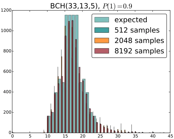
7.3 Application of the weight estimation algorithm by pro-cessing of a bit stream withP(1) = 0.1 by the generator
matrix of the BCH(33, 13, 5) code. . . 140
7.4 Application of the weight estimation algorithm by
pro-cessing of a bit stream withP(1) = 0.9 by the generator matrix of the BCH(33, 13, 5) code. . . 141
List of Tables
5.1 The sequences Ls fors= 1,2,3,4. . . 77
5.2 Bound B. . . 84
7.1 Some values of (d, n) for which Corollary 162 outper-forms some known bounds for binary codes. EB stands for Elias bound, JB for Johnson bound and HB for Hamming bound. . . 129
A.1 Bounds for codes withq = 2,d= 4, 3≤k≤28. . . 146
A.2 Bounds for codes withq = 2,d= 6, 3≤k≤30. . . 147
A.3 Bounds for codes withq = 2,d= 8, 3≤k≤30. . . 148
A.4 Bounds for codes withq = 2,d= 10, 3≤k≤30. . . . 149
A.5 Bounds for codes withq = 2,d= 12, 3≤k≤30. . . . 150
A.6 Bounds for codes withq = 2,d= 14, 3≤k≤30. . . . 151
A.7 Bounds for codes withq = 2,d= 16, 3≤k≤30. . . . 152
A.8 Bounds for codes withq = 2,d= 18, 3≤k≤30. . . . 153
A.9 Bounds for codes withq = 2,d= 20, 3≤k≤30. . . . 154
A.10 Bounds for codes withq = 2,d= 22, 3≤k≤30. . . . 155
A.11 Bounds for codes withq = 3,d= 6, 3≤k≤11. . . 156
A.12 Bounds for codes withq = 3,d= 7, 3≤k≤11. . . 156
A.13 Bounds for codes withq = 3,d= 8, 3≤k≤12. . . 157
A.14 Bounds for codes withq = 3,d= 9, 3≤k≤12. . . 157
A.15 Bounds for codes withq = 3,d= 10, 3≤k≤12. . . . 158
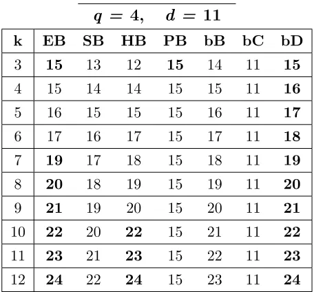
A.16 Bounds for codes withq = 3,d= 11, 3≤k≤12. . . . 158
A.17 Bounds for codes withq = 3,d= 12, 3 k 12. . . . 159
A.18 Bounds for codes withq = 3,d= 13, 3≤k≤12. . . . 159
A.19 Bounds for codes withq = 4,d= 9, 3≤k≤11. . . 160
A.20 Bounds for codes withq = 4,d= 10, 3≤k≤11. . . . 160
A.21 Bounds for codes withq = 4,d= 11, 3≤k≤12. . . . 161
A.22 Bounds for codes withq = 4,d= 12, 3≤k≤12. . . . 161
A.23 Bounds for codes withq = 4,d= 13, 3≤k≤12. . . . 162
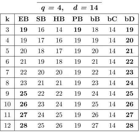
A.24 Bounds for codes withq = 4,d= 14, 3≤k≤12. . . . 162
A.25 Bounds for codes withq = 4,d= 15, 3≤k≤12. . . . 163
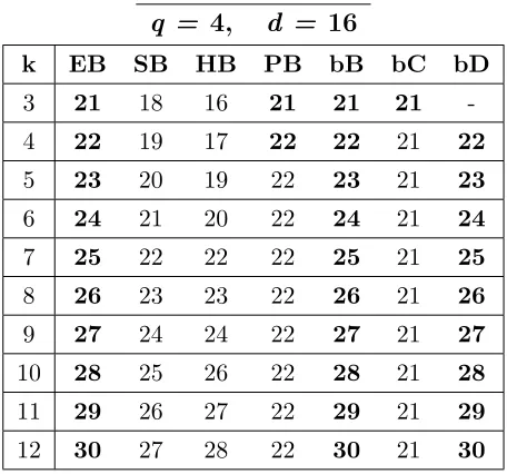
A.26 Bounds for codes withq = 4,d= 16, 3≤k≤12. . . . 163
A.27 Bounds for codes withq = 5,d= 11, 3≤k≤11. . . . 164
A.28 Bounds for codes withq = 5,d= 12, 3≤k≤11. . . . 164
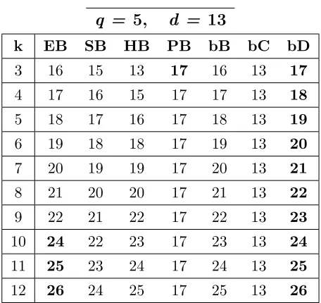
A.29 Bounds for codes withq = 5,d= 13, 3≤k≤12. . . . 165
A.30 Bounds for codes withq = 5,d= 14, 3≤k≤12. . . . 165
A.31 Bounds for codes withq = 5,d= 15, 3≤k≤12. . . . 166
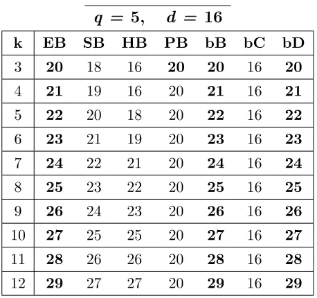
A.32 Bounds for codes withq = 5,d= 16, 3≤k≤12. . . . 166
A.33 Bounds for codes withq = 5,d= 17, 3≤k≤12. . . . 167
A.34 Bounds for codes withq = 5,d= 18, 3≤k≤12. . . . 167
A.35 Bounds for codes withq = 7,d= 15, 3≤k≤11. . . . 168
A.36 Bounds for codes withq = 7,d= 16, 3≤k≤11. . . . 168
A.37 Bounds for codes withq = 7,d= 17, 3≤k≤12. . . . 169
A.38 Bounds for codes withq = 7,d= 18, 3≤k≤12. . . . 169
A.39 Bounds for codes withq = 7,d= 19, 3≤k≤12. . . . 170
A.40 Bounds for codes withq = 7,d= 20, 3≤k≤12. . . . 170
A.41 Bounds for codes withq = 7,d= 21, 3≤k≤12. . . . 171
A.42 Bounds for codes withq = 7,d= 22, 3≤k≤12. . . . 171
A.43 Bounds for codes withq = 8,d= 17, 3≤k≤11. . . . 172
A.44 Bounds for codes withq = 8,d= 18, 3≤k≤11. . . . 172
A.45 Bounds for codes withq = 8,d= 19, 3≤k≤12. . . . 173
A.46 Bounds for codes withq = 8,d= 20, 3≤k≤12. . . . 173
A.47 Bounds for codes withq = 8,d= 21, 3≤k≤12. . . . 174
A.48 Bounds for codes withq = 8,d= 22, 3≤k≤12. . . . 174
A.49 Bounds for codes withq = 8,d= 23, 3≤k≤12. . . . 175
A.50 Bounds for codes withq = 8,d= 24, 3≤k≤12. . . . 175
Introduction
“
Information is the resolution of uncertainty.”
Claude Shannon
“
Truth emerges more readily from error than from confusion.”
Francis Bacon
Coding Theory deals with the problem of safe communication:
signals sent through a noisy channel can indeed be corrupted and
therefore reach their destination with some errors. In order to protect
the information content, some redundancy is added to the message,
so that the original data can be retrieved from corrupted signals. The
first example of a code is what is commonly known asrepetition code. Each symbol is repeated several times during transmission, in such a
way that the receiver can reconstruct the original message by selecting
the most probable one. A fundamental aspect, that arises from the
example above, is therefore how to achieve the desired correction
ca-pability while keeping the number of redundancy symbols small. This
problem is far from simple. We still do not fully know optimal codes,
and the study of what is possible to achieve is normally carried on by
presenting bounds on code parameters.
Another aspect of communication is privacy. Proofs of security
usu-ally rely on the utilisation of randomly picked keys which are used
to encrypt the data and have to be kept secret. The first step to
al-low secure communication is therefore to produce these random keys.
The most basic example of random number generator is the flip of a balanced coin. In the ideal case, each of the values associated to
the two sides of the coin can be generated with equal probability.
However, real world generators are not ideal and their outcomes are
not balanced. To improve the quality of the random keys we rely on
entropy extractors, compression functions designed to output random numbers from unbalanced sequences of bits.
In this work we deal with both safety and security of
communica-tion as introduced above.
Regarding Coding Theory, we start from a thorough analysis of known
bounds on code parameters and a study of the properties of Hadamard
codes. We find of particular interest the Griesmer bound, which is a
3
it to all codes, and we can determine many parameters for which the
Griesmer bound is true also for nonlinear codes. In case of systematic
codes, a class of codes including linear codes, we can derive stronger
results on the relationship between the Griesmer bound and optimal
codes. For example, we prove that the Griesmer bound holds for all
binary systematic codes whose distance is either a power of 2 or the
difference between two powers of 2. On the other hand, we construct a
family of optimal binary systematic codes contradicting the Griesmer
bound. Finally, we obtain new bounds on the size of optimal codes.
As for the study of random number generation, we analyse linear
ex-tractors and their connection with linear codes. The main result on
this topic is a link between code parameters and the entropy rate
ob-tained by a processed random number generator. More precisely, to
any linear extractor we can associate the generator matrix of a linear
code. Then, we link the total variation distance between the uniform
distribution and the probability mass function of a random number
generator with the weight distribution of the linear code associated to
the linear extractor.
Finally, we present a collection of results derived while pursuing a way
to classify optimal codes, such as a probabilistic algorithm to compute
the weight distribution of linear codes and a new bound on the size
of codes.
This work is organised as follows. Chapters1to4contain the back-ground on Coding Theory and Random Number Generation needed
for the research presented in Chapters5,6 and7.
Chapter 1 describes basic results and definitions on Coding Theory, with focus on nonlinear codes. In Chapter2we present an overview of
the most known bounds on code parameters, such as the Sphere
pack-ing bound, the Gilbert bound, the Varshamov bound, the Spack-ingleton
bound, the Griesmer bound, the Plotkin bound, the Johnson bound,
Bellini-Guerrini-Sala bounds. Then in Chapter3 we discuss Hadamard ma-trices and their link with optimal nonlinear codes. In Chapter 4 we introduce the theory behind Random Number Generation and entropy
extraction, following the definitions proposed by NIST.
Chapters5 to7 contain results on optimal codes and on entropy
ex-traction. Chapter 5 deals with optimal nonlinear systematic codes. In this chapter we study properties on codes useful to understand
the applicability of the Griesmer bound. These properties lead to a
classification of parameters for which we can apply the bound. Some
examples are:
• all codes whose distance is d≤2q,
• all codes for which the dimension k and the distance d satisfy
qk−1|d,
• all binary codes for which the minimum distance is either 2r or
2r−2s for any choice of positive integerss < r.
In the same chapter we analyse optimal binary codes with small
di-mension. Our main results are a complete classification of optimal
codes of dimension 2 and a collection of properties of codes of
dimen-sion 3. The analysis of optimal codes with respect to the Griesmer
bound is then concluded by presenting a new family of optimal
non-linear systematic binary codes contradicting the bound. This family
is obtained by using similar methods to the Levenshtein’s
construc-tion of optimal codes from Hadamard matrices. For eachk >3 these
codes are 2k+1+ 2,2k,2k+ 22 systematic codes, while the Gries-mer bound for codes of dimensionk and distance 2k+ 2 gives length
n≥2k+1+k−1.
Chapter 6 deals with entropy extractors. Previously known results showed a link between linear extractors and the minimum distance
of the codes generated by the same matrix used for the extraction
5
spectrum of the output of a binary random number generator and
the bias of individual bits, and use this to explain how previously
known bounds on the performance of linear binary codes as RNG
post-processing functions can be derived as a special case. We then
extend this framework to the case of output in non-binary finite fields
by use of the Fourier transform.
In Chapter7 we describe a probabilistic algorithm for computing the weight distribution of linear codes obtained by using methods derived
from our study on entropy extractors. Then we present some results
on polynomials in F2[X], such as a closed formula to compute the
binary M¨obius transform of a Boolean function and an equivalent
formulation of the Hilbert’s Nullstellensatz for the particular case of
Part I
Codes and Random
Chapter 1
Introduction to Coding
Theory
“
Frequently the messages have meaning; that is they re-fer to or are correlated according to some system withcertain physical or conceptual entities. These
seman-tic aspects of communication are irrelevant to the
en-gineering problem. The significant aspect is that the
actual message is one selected from a set of possible
messages.
”
Claude Shannon
In this chapter we introduce all concepts and notations we need
to present the main results of this work. Most of the definitions and
statements presented here are well known in literature and form the
basics of Coding Theory.
The theory presented in this work is not a complete introduction to
Coding Theory and we take for granted that readers have a basic
knowledge of linear algebra and finite fields. Therefore we list here
only some relevant properties and definitions, for a thorough
under-standing of the subject see e.g. [32]. Regarding Coding Theory, over this entire work we refer to classical books, as for example [22], [23],
[33] and [42].
We use as notation q to denote a prime power pm, Fq to denote
the finite field of sizeq and (Fq)n for the vector space of dimensionn
overFq. Whenever not otherwise specified, all vectors are considered
to be row vectors. This implies for example that linear maps between
vector spaces can be thought as right-multiplications by matrices.
Given two vectors u, v ∈ (Fq)n, we denote with w(u) the Hamming
weight ofu and with d(u, v) the Hamming distance between uand v.
We often call them simplyweight and distance. Proper definitions of weight and distance are the following.
Definition 1. Let u ∈ (Fq)n. The Hamming weight w(u) is the
number of non-zero coordinates ofu.
Definition 2. Letuandvbe in (Fq)n. The Hamming distance d(u, v)
betweenu andv is the number of coordinates in which they differ.
From Definition2it follows that d(u, v) = w(u−v). On the other
hand, w(u) can be seen as the distance betweenuand the zero vector.
Definition 3. Given a vectoru∈(Fq)nof weights, thesupportofuis
the set ofsindices supp(u) ={j1, . . . , js}for which the corresponding
11
The support of a vector u is therefore linked to its weight by the
formula w(u) =|supp(u)|.
Consider now two vectors u ∈ (Fq)n1 and v ∈ (Fq)n2. We define
the concatenation of u and v as the vector (u|v) ∈ (Fq)n1+n2 whose
firstn1 coordinates are the coordinates ofu while the lastn2 are the
coordinates ofv.
Definition 4. A code C is a set of M vectors in the vector space (Fq)n, whereFq is the finite field withq elements. We refer to each of
these vectors as acodeword c∈C, to nor len(C) as the length of C
and toM or |C|as its size.
We denote with d(C) or simply withd the minimum distance of C,
i.e. the minimum among the Hamming distances between any two
distinct codewords inC. A code C with such parameters is denoted
by the four parameters (n, M, d)q, or as an (n, M)q code whenever its
distance is unknown or not relevant.
Given a code, we can define its weight distribution and distance
distribution as follows.
Definition 5. Let C be an (n, M, d)q code. The weight distribution
ofC is the sequence of integers{Ai}i=0,...,n, where
Ai=|{c∈C : w(c) =i}|.
In the same way, thedistance distribution {Bi}i=0,...,n of C is defined
as
Bi=|{(c1, c2) : c1, c2 ∈C, d(c1, c2) =i}|.
We say that two codesCandC0are equivalent if there is a bijection
ϕ:C→C0which preserves the distances between any two codewords:
C∼C0 ⇐⇒ d (c1, c2) = d (ϕ(c1), ϕ(c2)), ∀c1, c2∈C.
In particular, translations by fixed vectors, multiplications by
permu-tation matrices and field permupermu-tations are maps which preserve the
Lemma 6. Let θbe a permutation of Fq and letϕ: (Fq)n→(Fq)n be
• a translation by a constant vector v∈(Fq)n,
• the multiplication by a permutation matrix P or
• the application of θ to the first coordinate of (Fq)n.
ThenC0 =ϕ(C) is a code equivalent to C.
Proof. By applying Definition2it is straightforward to prove the first two items. For the third point, let observe that for any bijectionθwe
haveα6=β if and only if θ(α)6=θ(β).
By combining functions as in Lemma 6 we obtain the following
proposition.
Proposition 7. Let θ1, . . . , θn be permutations of Fq, P an n×n permutation matrix andv∈(Fq)n a chosen vector. Then ϕ: (Fq)n→
(Fq)n defined by
ϕ(c) = (θ1(c1), . . . , θn(cn))·P+v,
withc= (c1, . . . , cn)∈(Fq)n, is a map which preserves the Hamming distances between vectors.
Let us denote with kthe minimum integer allowing the existence
of a mapF between (Fq)k and (Fq)n whose image isC itself, and let
us call it thecombinatorial dimension of C. Sometimes we also use dim(C) to denote the combinatorial dimension of the codeC. Clearly,
dim(C) is equal to
logqM
.
SinceF is a vectorial function, we can write
F(X) = (f1(X), . . . , fn(X)).
Definition 8. We callF agenerator function of the code. The maps
13
In the general case, the number of possible generator functions of
a code is given by
(
qk
M
)
·M!,
where
(
a
b
)
is the Stirling number of the second kind
(
a
b
)
= 1
b!
b
X
j=0
(−1)b−j
b j
ja.
In the particular case ofM =qk, the number of functions reduces to
M!.
Definition 9. C is alinear code ifCis a vector subspace of (Fq)n. In
this case,M =qkfor a certain positive integerkcalled thedimension
of the code. Notice thatkcoincides with the combinatorial dimension
ofC.
A linear code is denoted as an [n, k]q code, and with [n, k, d]q code
whenever its distance is known.
The number of generator functions of a linear code is therefore
M! = qk!, and among these there is at least a map F for which all
f1, . . . , fn are linear maps. In this case F becomes the multiplication
by ak×nmatrix Gwith coefficients in the field, which is known as thegenerator matrix ofC.
Example 1. LetC be the [3,2,2]2 linear code
C={c0, c1, c2, c3}={(0,0,0), (1,1,0), (0,1,1), (1,0,1)}.
A possible generator function is given by
F(0,0) = (1,1,0), F(1,0) = (0,0,0), F(0,1) = (0,1,1), F(1,1) = (1,0,1),
which is the vectorial Boolean function
wheref1, f2 andf3 are therefore defined by
f1(0,0) = 1, f2(0,0) = 1, f3(0,0) = 0,
f1(1,0) = 0, f2(1,0) = 0, f3(1,0) = 0,
f1(0,1) = 0, f2(0,1) = 1, f3(0,1) = 1,
f1(1,1) = 1, f2(1,1) = 0, f3(1,1) = 1,
and can be explicitly obtained through the binary Moebius transform, as shown in Section7.2. We have
F(x1, x2) = ( 1 +x1+x2, 1 +x1, x2).
Notice now that even thoughCis linear,F is a not a linear function. How-ever, given σa permutation of (F2)
2
, the image of the function ¯F =F ◦σ
is again a generator function for the same code C, since the image of ¯F
coincides with the image ofF.
By choosing for exampleσ(x1, x2) = (x1+ 1, x2) we obtain
¯
F(x1, x2) = (x1+x2, x1, x2),
to which is associated the generator matrix
G=
"
1 1 0 1 0 1
# .
Notice that in example 1 the map F was an affine function. In the general caseF could be a nonlinear map, even though its image
is a linear code. This however cannot happen with binary codes of
dimension 2 in which the evaluation vectors of the functionsf1, . . . , fn
have even weight.
Definition 10. A code which is not equivalent to any linear code is called astrictly nonlinear code.
Proposition 11. The evaluation vectors of the non-constant compo-nents of a linear code are balanced, namely each α ∈ Fq appears Mq times. MoreoverM has to be a power ofq.
When considering linear codes, there is no need to consider both
the weight distribution and the distance distribution. The first
15
code. This follows directly from Definition9. Moreover, the minimum distance of a linear code coincides with the minimum of the weight
distribution. The proof relies again on the definition itself of linear
code: ifc1 andc2 are two codewords at minimum distance, their
dif-ference is a codeword at minimum distance from the zero codeword,
namely a codeword of minimum weight.
Since a linear codeCis a vector subspace of (Fq)nwe can consider
its dual, which is the vector subspace of (Fq)n whose elements are
orthogonal toC. The dual code of C coincides with the kernel of any its generator matrix, hence its dimension isn−dim(C).
Example 2. LetC be the binary linear code generated by the matrix
G=
"
1 1 0 1 0 1
# ,
as in Example1. The kernel ofGis the vector subspaceh(1,1,1)i, meaning that the dual ofC is the code generated by the matrix
H =h1 1 1
i .
Definition 12. Thedual of a linear codeC is the linear code whose codewords are orthogonal to C. The dual of C is denoted as C⊥
and its generator matrix is usually denoted as H. H is called the
parity-check matrix of C,
By using the parity-check matrix, it is possible to prove several
interesting properties of linear codes. Other than the following known
result, we will use parity-check matrices also to show the link between
puncturing and shortening of codes in Section1.2.
Proposition 13. Let C be an [n, k]q linear code and let H be its parity-check matrix. Then d(C) = d if and only if the minimum number of linear dependent columns ofH is d.
Proof. Ifc∈C is a codeword of minimum weight d, then H·ct= 0. This means that there is a linear relation between the columns of H
For notation purposes, we will often use the following non standard
definition.
Definition 14. Let C be an (n, M)q code. We call codebook of C
any M ×n table whose M rows are the codewords of C. With a
slight abuse of notation, we will often denote a codebook of C with
the symbolC itself.
Codebooks are usually associated to nonlinear codes for encoding
procedures. Indeed, we remark that the choice of a codebook forC is
equivalent to order its codewords. Clearly, permutations of the rows
of a codebook lead to other codebooks of the same code, in the same
manner in which there exist several generator functions for the same
code. Field permutations applied to the columns ofC, permutations
of its columns and translations of its rows by a single fixed vector of
(Fq)n lead to equivalent codes.
Once a codebook has been chosen we have a table
C={ci,j}i=0,...,M−1, j=1,...,n,
so we will denote with ci the i-th codeword of C, which is the i-th
row of its codebook, and withci,j its j-th coordinate.
In the next section we present systematic codes, a family of codes
containing linear codes.
1.1
Definition of systematic codes
Systematic codes form an important family of nonlinear codes. As
we will show in Chapter 5, in the general case systematic codes can achieve better error correction capability than any linear code with
the same parameters. On the other hand, due to their particular
structure, systematic codes can achieve faster encoding and decoding
procedures than nonlinear non-systematic codes. Moreover, many
1.1. Definition of systematic codes 17
Definition 15. An (n, qk, d)qsystematic codeCis the image of an
in-jective mapF : (Fq)k→(Fq)n,n≥k, s.t. a vectorX= (x1, . . . , xk)∈
(Fq)k is mapped to a vector
(x1, . . . , xk, fk+1(X), . . . , fn(X))∈(Fq)n,
where the fi are maps from (Fq)k toFq. The coordinates from 1 to
k are called systematic, while those from k+ 1 to n are called non-systematic.
A more general statement defines systematic codes as nonlinear
codes equivalent to those described in Definition15.
Definition 16. LetCbe an (n, qk, d)qcode, and let F = (f1, . . . , fn)
be a generator function ofC. C is a systematic code if there exist k
indicesi1, . . . , ikfor which the function (fi1, . . . , fik) is a permutation
of (Fq)k.
According to Definition15, any linear code is equivalent to a sys-tematic code. The proof involves permutation of the columns of its
generator matrix and application of the Gauss reduction to its rows.
In this way we can find an equivalent code for which the generator
matrixGis in the form
G=hIk | Rn−k
i
,
whereIk is the identity of order kand Rn−k is ak×(n−k) matrix.
By applying instead Definition 16, each linear code can directly be
called a systematic code.
Proposition 17. Let C be a systematic code as in Definition 15. ThenC is a linear code if and only if the componentsfk+1, . . . , fn are linear functions.
Proof. If fk+1, . . . , fn are linear maps and c1, c2 are in C, then both
On the other hand, if a componentfjis not linear, then there exist two
vectorsa= (a1, . . . , ak) andb= (b1, . . . , bk) for whichfj(a) +fj(b)6=
fj(a+b) and this implies that C is not a linear code.
1.2
Puncturing, shortening and extending
The three most simple and common ways of obtaining new codes
starting from known ones are
• puncturing,
• shortening and
• extending.
In this section we briefly describe these methods and we discuss some
of the properties of the obtained code with respect to the parameters
of the known code.
Definition 18. Puncturing a code C in the j-th coordinate means deleting from all codewords of C the j-th coordinate. We denote
with ˙Cj1,...,js the code obtained by puncturing C in the coordinates
j1, . . . , js, or simply with ˙Cwhenever we do not need to specify which
coordinates were punctured.
The following proposition links the generator functions of ˙Cj to
the generator function ofC, and follows directly from Definition18.
Proposition 19. Let F = (f1, . . . , fj−1, fj, fj+1, . . . , fn) be a gener-ator function of a codeC.
ThenF˙j = (f1, . . . , fj−1, fj+1, . . . , fn) is a generator function for C˙j.
Given two codewordsc1, c2∈Cand the corresponding codewords
˙
c1 and ˙c2 in ˙Cj, we have
d( ˙c1,c˙2) = d(c1, c2) ifc1,j=c2,j
1.2. Puncturing, shortening and extending 19
As a consequence, by puncturingC in a single coordinate, we find ˙C
whose distance is either equal to d(C) or to d(C)−1. In particular,
d( ˙Cj) = d(C) if and only if the componentfj is a constant function.
Let us consider now two codewords c1 and c2 in C at minimum
distance d, and let supp(c1 −c2) = {j1, . . . , jd}. The puncturing of
C in the coordinates j1, . . . , jd is a code with strictly less than M
codewords. The proof of this is a straightforward consequence of the
fact that both c1 and c2 are equal in all coordinates non indexed by
elements in supp(c1−c2), namely in ˙Cj1,...,jd we have ˙c1 = ˙c2. Let C
be an [n, k, d]q linear code, and c,c¯∈ C with ¯c of minimum weight
d. From the linearity of C it holds that c+αc¯∈C for each α∈Fq,
and these q codewords become the same after puncturing C in the
coordinates supp(¯c). It follows that, by puncturing a linear code C
in the support of a codeword of minimum weight, we obtain a new
linear code whose dimension is strictly less than dim(C).
Definition 20. Let C be an (n, M, d)q code. Shortening C in the j-th coordinate means to consider the subset S of C containing all
codewords whosej-th coordinate is equal zero, and then puncturing
S in thej-th coordinate.
We denote with ¨Cj1,...,js the code obtained by shortening C in the
coordinatesj1, . . . , js, or simply with ˙C whenever we do not need to
specify which coordinates were shortened.
Similar to puncturing, shortening a code C produces a new code
whose length is len(C)−1. On the other hand, the definition of
short-ening implies that the distance of ¨C is at least equal to the distance
ofC. Any pair of codewords in ¨Cj correspond to a pair of codewords
in C whose j-th coordinates are equal, hence the shortening cannot
have decreased their mutual distance.
Regarding the size of ¨C, things are more complicated than with
punc-turing. First, if the j-th component of C is the constant 0, then
code. On the other hand, if thej-th coordinate is different from 0 for
all codewords, then ¨Cj =∅.
In the general case, we have the following result.
Proposition 21. Let C be an (n, M)q code with distance larger than
1, and letθα be a permutation of Fq which map α to 0.
We consider the set {Cα} of equivalent codes obtained from C by applyingθα to thej-th coordinate ofC for each α∈Fq. We consider the set of codesS=nC¨α
o
α∈Fq
obtained by shortening the codes{Cα} in the j-th coordinate. Then
1. the codes in S are disjoint, meaning that a codeword cannot belong to more than one code in the set.
2. The union of all codes in S is the codeC˙j.
3. There is at least anα∈Fq such that
¨
Cα
≥
M q . Proof. Without loss of generality, let us assume that j=n.
1. If a codeword ¨c belongs to more than a single code in S, then
the concatenation (¨c|0) belongs to more than a code in {Cα},
sayCα and Cβ. This means that both (¨c|α) and (¨c|β) are inC,
hence the minimum distance of C is 1.
2. If ¨cis in ¨Cα, then (¨c|α)∈C. Moreover, if (¨c|α) is a codeword of
C, then ¨c∈C¨α. This implies that by joining the codes inS we
obtain the set of all codewords in C to which we have removed
the last coordinate, and this is the definition of ˙C.
3. Follows directly from |C| = M and points 1. and 2. of this
proposition.
If we consider linear codes we have a deeper characterisation given
1.2. Puncturing, shortening and extending 21
Proposition 22. Let C be an [n, k, d]q linear code and let D =C⊥ the dual of C. Then
1. len( ¨C) =n−1;
2. d( ¨C)≥d;
3. if the j-th component of C is the constant 0, then C¨j = ˙Cj. In particular the dimension of C¨ is k.
4. if the j-th component of C is not constant, then the dimension of C¨j isk−1.
5. C¨j =
˙
Dj
⊥
.
Proof. 1. It follows directly from the definition of shortening.
2. The codewords in ¨C are obtained by puncturing a subset of
C containing elements whosej-th coordinate is equal 0. Since
this set is contained in C, its codewords are at distance at least
d, hence by deleting a coordinate which is constantly 0 their
pairwise distances cannot decrease.
3. ¨Cj is by definition the puncturing of the subcode ofC consisting
of codewords whose j-th coordinate is 0. If all codewords in C
possess this property, then shortening and puncturing lead to
the same code. Moreover, the size of ¨C is equal to the size ofC.
4. Since thej-th component ofCis linear, then its evaluation
vec-tor is balanced, namely each α ∈ Fq appears the same amount
of times, i.e. |Cq| = qk−1. This holds in particular for α = 0,
hence |C¨j|=qk−1.
5. Dcontains all vectors in (Fq)nwhich are orthogonal to the
code-words in C. Let us consider a codewordc∈C whosej-th
does not depend on thej-th coordinate of ¯c, hence by
punctur-ing both c and ¯cin the j-th coordinate we still obtain a pair of
orthogonal vectors. This imply that by puncturing in the j-th
coordinate both the set of codewords inCwhosej-th coordinate
is 0 andDwe obtain two orthogonal codes. To prove that these
two codes, namely ¨Cj and ˙Dj, are dual codes we observe that
dim ¨Cj = dim
˙
Dj
⊥
.
Proposition 23. Let C be an (n, qk, d)q systematic code, and C0 be the code obtained by shortening C in a systematic coordinate. Then C0 is an (n−1, qk−1, d0)q systematic code withd0 ≥d.
Proof. To obtainC0, consider the code
C00 =nF(X)|X= (0, x2, . . . , xk)∈(Fq)k
o
,
i.e. the subcode ofC which is the image of the set of messages whose
first coordinate is equal to 0. ThenC00 is such that dim(C00) =k−1
and d(C00) ≥ d. Since, by construction, all codewords have the first
coordinate equal to zero, we obtain the codeC0 by puncturingC00 on
the first coordinate, so that
(
len(C0) =n−1
d0= d(C0) = d(C00)≥d.
Lemma 24. For any (n, qk, d)
q systematic code C, there exists an
(n, qk,d¯)q systematic code C¯ for any1≤d¯≤d.
Proof. Since n > k, we can consider the code C1 obtained by punc-turing C in a non-systematic coordinate. C1 is an (n−1, qk, d(1))q
systematic code. Of course, eitherd(1) =dord(1) =d−1.
By puncturing at mostn−knon-systematic coordinates, we will find
1.2. Puncturing, shortening and extending 23
that the codeCi, obtained by puncturing C in the lasticoordinates,
has distance equal to ¯d. Once the (n−i, qk,d¯) codeCi has been found,
we can obtain the claimed code ¯Cby paddingizeros to all codewords
inCi.
The proofs of Proposition23and Lemma24rely on the systematic
property of C, hence they hold for linear codes as well. For
non-systematic codes we have the following more general statement.
Lemma 25. For any (n, M, d)q code C, there exists an (n, M,d¯)q code C¯ for any 1≤d¯≤d.
Proof. By proceeding in a similar manner as in the proof of Lemma
24, we punctureC till we reach a code whose distance is ¯d. Then ¯C is
obtained by padding the necessary amount of zeros to all codewords
of the punctured code.
We conclude this section with the notion of extension of a code.
The idea is to add a new coordinate to a codeC, hopefully increasing
its distance. The definition of the new component is given in terms of
the components ofC, so in general it is a map (Fq)n →Fq evaluated
at the components of C. The result is therefore a map (Fq)k → Fq
which is used as the new component.
By the definition above, there are several possible ways to define an
extension of a code - as much as the maps (Fq)k→Fq - however the
new-added component is usually defined by
fn+1 =−
X
j
fj. (1.1)
In this work we will always refer to this particular type of extension
as the extension ofC.
Definition 26. Let C be a code with length n, let f1, . . . , fn be its
components and let fn+1 be as in equation (1.1). We denote with
E(C) the extension ofC defined by the components
Notice thatfn+1 is the composition between a linear function and
the components ofC. This lead to the following results.
Proposition 27. E(C) is linear if and only if C is a linear code.
Proof. IfE(C) is linear then its components are linear. In particular
f1, . . . , fn are linear functions, so the components of C are all linear
functions. For the other way around, iff1, . . . , fnare linear, then also
fn+1 =−Pnj=1fj is a linear function, makingE(C) a linear code.
Proposition 28. The distance of E(C) is either equal to d(C) or
d(C) + 1.
Proof. The distance ofC cannot decrease after an extension, and by adding a single coordinate it cannot increase by more than 1.
Proposition 29. The sum of the coordinates of each codeword in E(C) is 0.
Proof. It follows directly from the definition ofE(C).
Proposition 29 lead to very interesting properties, mainly in the case of binary codes, as stated by the following results.
Corollary 30. Let C be a binary code. Then E(C) contains only codewords of even weight.
Proof. It follows from Proposition 29. A binary codeword has even weight if and only if the sum of its coordinates is 0.
Proposition 31. Let C be an (n, M, d)2 code with odd distance d. ThenE(C) has distance equal tod+ 1.
Proof. By Corollary 30 in E(C) there are only codewords with even weight, and the distance between two such codeword cannot be odd.
1.2. Puncturing, shortening and extending 25
In the general case, extending and puncturing do not commute,
i.e. while it is true that by extending and then puncturing a code
C we obtain againC, it is not true that extending a punctured code
will lead to the original code. In the following proposition we assume
without loss of generality that both extending and puncturing are
referred to the last coordinate of the code.
Proposition 32. Let C be a code. Then
1. E˙(C) =C ,
2. E( ˙C)6=C , and
3. in the linear binary case E( ˙C) = C if and only if C has only codewords of even weight.
Chapter 2
Bounds on code
parameters
“
It may seem surprising that we should define a defi-nite capacity C for a noisy channel since we can neversend certain information in such a case. [...]
Na-ture takes payment by requiring just that much
uncer-tainty, so that we are not actually getting any more
than C through correctly.
”
Claude Shannon
A classical problem in coding theory is to determine the
parame-ters of optimal codes, and this characterisation is usually carried on
by presenting bounds on the minimum distance, on the size, or on the
length of codes. Since two equivalent codes have the same parameters,
we can always assume that the zero codeword belongs toC.
In this chapter we present an overview of the most common bounds
on the size of a code. Most bounds estimate the maximum number
of codewords in a code whose length and distance are known. This
is not the case for the Griesmer bound, whose classical description
gives a lower-bound on the length of a linear code with given size and
minimum distance. We will discuss extensively the Griesmer bound
in Chapter5.
Definition 33. We denote with
• Aq(n, d) the maximum size of a nonlinear code whose length is
n and whose distance isd.
• Bq(n, d) the maximum size of a linear code whose length is n
and whose distance is d.
• Nq(M, d) the minimum length of a nonlinear code whose size is
M and whose minimum distance isd.
• Sq(k, d) the minimum length of a nonlinear systematic code with
dimension kand minimum distance d.
• Lq(k, d) the minimum length of a linear code with dimensionk
and minimum distance d.
Clearly there exist some relations between these values, as
ex-plained by the following proposition.
Proposition 34. Bq(n, d) ≤ Aq(n, d) and Nq(M, d) ≤ Sq(k, d) ≤ Lq(k, d).
2.1. Sphere packing bound 29
Definition 35. We denote with Sr(x) the Hamming sphere centred
atxof radiusr, and with Volq(n, r) =
Pr i=0
n i
(q−1)i the volume of
a sphere in (Fq)n of radius r.
2.1
Sphere packing bound
The sphere packing bound, also known as Hamming bound, is a
first and very important bound on the size of a code and was
pro-posed in 1950 by R. W. Hamming [19]. Codes meeting the sphere packing bound are calledperfect codes. In a perfect code the spheres of radiust=n−1
2
centred at codewords cover the entire space (Fq)n,
or equivalently for each vector v in the space the sphere or radius t
contains a codeword. This imply that each vector can be successfully
decoded without ambiguity.
Theorem 36 (Sphere packing bound).
Bq(n, d)≤Aq(n, d)≤ qn
Volq(n, t) ,
where t=d−21.
Proof. Given an (n, M, d)q code, theM spheres of radiustcentred at
theM codewords are pairwise disjoint.
2.2
Gilbert bound
The following result is a lower bound on the size of a code proposed
in 1952 by E. N. Gilbert [12]. The covering radiusρ(C) of an (n, M, d)q
code is the minimum integer r such that the union of the spheres of
radiusrcentred at theM codewords is equal to the entire space (Fq)n.
An argument similar to the proof of the Sphere packing bound leads
Theorem 37 (Gilbert bound).
Aq(n, d)≥Bq(n, d)≥
qn
Volq(n, d−1)
Proof. The covering radius of an [n, Bq(n, d), d]q linear code C is at
mostd−1. The proof of this fact is by contradiction. Suppose there
exists an element of (Fq)n at distance at least d from any codeword
inC. In this case we could construct another linear code ¯C with the
same length and distance as C, and dimension strictly larger than
Bq(n, d), which leads to the claimed contradiction.
Since the spheres of radiusd−1 centred at the codewords ofC cover
(Fq)n, it follows thatBq(n, d) is at least equal to the number of such
spheres, and the result follows.
2.3
Varshamov bound
Another lower bound forBq(n, d) was proposed in 1957 by R. R.
Varshamov [50].
Lemma 38. Let n, k and d be integers such that 2 ≤ d ≤ n and
1≤k≤n, and let q be a prime power. If
d−2
X
i=0
n−1
i
(q−1)i< qn−k, (2.1)
then there exists ann−k×nmatrixH over Fq such that every d−1 columns ofH are linearly independent.
Proof. We use the following algorithm to find thencolumnsh1, . . . , hn
ofH. Notice that each column is a vector in (Fq)n−k. Choose:
• h1 to be any nonzero vector;
• h2 to be any vector which is not a multiple ofh1;
• hj to be any vector which is not a linear combination ofd−2
2.4. Singleton bound 31
If we can carry out this algorithm to completion, then h1, . . . , hn are
the columns of ann−kby nmatrix with the wanted property.
Suppose we have found h1, . . . , hj, with 1 ≤ j ≤ n. The number of
linear combinations ofd−2 or fewer ofh1, . . . , hj is
d−2
X i=0 j i
(q−1)i≤ d−2
X
i=0
n−1
i
(q−1)i.
Hence if equation (2.1) holds, then there is some vectorhj+1 which is not a linear combination ofd−2 (or fewer) ofh1, . . . , hj. By induction
we conclude.
H can be considered as the parity check matrix of a linear codeC
of lengthnand dimension at leastk. Since everyd−1 columns ofH
are linear independent,C has distance at leastdby Proposition 13.
Corollary 39. Let n, k and d be integers such that 2 ≤d ≤n and
1 ≤ k ≤ n. Then there exists an [n, k]q linear code with minimum distance at least d, provided that
1 +
d−2
X
i=0
n−1
i
(q−1)i≤qn−k. (2.2)
Theorem 40 (Varshamov bound).
Bq(n, d)≥qn−dlogq(1+
Pd−2
i=0(
n−1
i )(q−1) i)e
.
Proof. The largest integerk satisfying equation (2.2) is equal to
$
n−logq 1 +
d−2
X
i=0
n−1
i
(q−1)i
!%
,
hence the theorem follows from Corollary39.
2.4
Singleton bound
One of the most commonly used bounds was presented in 1964 by
Maximum Distance Separable (MDS) codes, and are of great
impor-tance in both Coding Theory and Cryptography.
Theorem 41 (Singleton bound).
Aq(n, d)≤qn−d+1.
Proof. By puncturing an (n, M, d)q code in d−1 coordinates, we
obtain an (n, M)q code with distance at least 1, henceM is at most
qn−d+1.
By applying the Singleton bound to linear codes we obtain the
following corollary.
Corollary 42(Singleton bound for linear codes). LetCbe an[n, k, d]q linear code. Then
k≤n−d+ 1.
Let consider now an [n, k, d]qcodeC. IfDis any subcode ofC, we
define the support supp(D) of D as the set of coordinates where not
all the codewords ofDare zero. Equivalently, the support ofDis the
set of indices corresponding to the nonzero columns of the generator
matrix ofD.
For 1≤r≤k, the r-th-generalized Hamming Weight of C is defined
as
dr(C) =dr= min{|supp(D)| |Dis an [n, r] subcode of C}.
Notice that
d=d1< d2 < . . . < dk≤n,
and the set {d1, . . . , dk} is called the weight hierarchy of C. The
weight hierarchy is invariant under any monomial map applied toC.
Theorem 43 (Generalized Singleton bound). Let C be an [n, k, d]q linear code. For1≤r≤k
2.5. Griesmer bound 33
Proof. It follows by induction onk−r, starting withdk≤nand using d1 < . . . < dk.
2.5
Griesmer bound
The Griesmer bound, which can be seen as an extension of the
Singleton bound [23, Section 2.4] in the linear case, was introduced by Griesmer [14] in the case of binary linear codes and then
general-ized by Solomon and Stiffler [45] in the case of q-ary linear codes. It is known that the Griesmer bound is not always sharp [34], [35], [49]. Important examples of linear codes meeting the Griesmer bound are
the simplex code [23, Section 1.3] and the [11,5,6]3 Golay code [13], [23, Section 1.12].
Definition 44. Let C be a linear code, and let c ∈ C. We denote with Res(C, c) the residual code of C with respect to c, namely the
linear code obtained by puncturingC in the nonzero coordinates ofc.
Lemma 45. If C is an [n, k, d]q code and c ∈C has weight d, then
Res(C, c) is an [n−d, k−1,d˙]q code where d˙≥
l
d q
m
.
Proof. By replacing C with an equivalent code, we can assume c = (1, . . . ,1,0, . . . ,0), namely, the nonzero coordinates of c are the first
dcoordinates.
First, we prove that the dimension of Res(C, c) is k−1. Assume
that this is not true, which means that the dimension is strictly less
thank−1. Then there exists a nonzero codeword x∈C of the form
x= (x1, . . . , xd,0, . . . ,0), and x is not a multiple of c. Observe that
x1, . . . , xdare nonzero, otherwise the weight ofxwould be strictly less
thand. We consider now the codeword x1·c= (x1, . . . , x1,0, . . . ,0)
which belongs toCdue to the linearity ofC. Thend(x, x1·c)< d, and
we have a contradiction. Hence the dimension of Res(C, c) is k−1.
Res(C, c), and letu∈(Fq)dbe such that the concatenation (u|v)∈C.
Observe that there exists anα∈Fqsuch that at leastd/qcoordinates
ofu equalα. Then
d≤d((u|v), α·c)≤d−d
q +w(v),
from which it follows that
w(v)≥ d q.
Since this is true for all codewords in Res(C, c), then ˙d≥ dq.
Theorem 46 (Griesmer bound). Let k≥1. Then
Lq(k, d)≥ k−1
X
i=0
d qi
.
Proof. Consider an [n, k, d]q code. The proof is by induction on k. If k = 1 the conclusion holds. Assume that k > 1 and let c ∈ C be
a codeword of weight d. By Lemma 45 the residual code Res(C, c)
is an [n−d, k −1,d˙]q code with ˙d ≥
l
d q
m
. Applying the inductive
assumption, we have
n−d≥ k−2
X
i=0
d qi+1
.
2.6
Plotkin bound
The following is an upper bound due to M. Plotkin, first present
in 1960 [39]. Binary codes meeting the Plotkin bound are of great importance for several reasons. First, it seems that for each (n, d)
pair there exists a code whose size meets the bound. Furthermore,
optimal codes in the Plotkin range are equidistant codes, i.e. each
pair of codewords is at distance exactly d. Finally, as we will see in
2.6. Plotkin bound 35
Theorem 47(Plotkin bound). Let C be an (n, M, d)q code such that rn < d, withr= 1−q−1. Then
M ≤
d d−rn
Proof. Consider S = P
x∈C
P
y∈Cd(x, y). Since d(x, x) = 0, while d(x, y)≥dfor each pairx6=y, it follows that
M(M−1)d≤S. (2.3)
LetA be a codebook forC. For 1≤i≤n, let ni,α be the number of
timesα∈Fq occurs in the i-th column ofA. We have
S = n X i=1 X α
ni,α(M −ni,α) =nM2− n
X
i=1
X
α n2i,α.
Using the Cauchy-Schwartz inequality, we observe that
X
α
n2i,α=q−1 X α
n2i,α
! X
α
1
!
≥q−1 X α
ni,α
!2
,
hence
S≤nM2− n
X
i=1
q−1 X α
ni,α
!2
.
SinceP
αni,α=M, we have
S≤nM2−nq−1M2=nM2 1−q−1=nrM2. (2.4)
Combining equations (2.3) and (2.4) we obtain
M(M −1)d≤nrM2,
from which we have
M(d−rn)≤d.
• If dis even and n <2d, A2(n, d)≤2
j
d 2d−n
k
.
• If dis even, A2(2d, d) = 4d.
• if d is odd andn <2d+ 1, A2(n, d)≤2
j
d+1 2d+1−n
k
.
• If dis odd, A2(2d+ 1, d) = 4d+ 4.
2.7
Johnson bounds
Another remarkable result is due to S. Johnson [24]. In 1962 he
presented a new upper bound by examining binary constant-weight
codes, namely codes in which all codewords have the same Hamming
weight. DefineA2(n, d, w) to be the maximum number of binary
code-words of lengthnand weightwwhich are distant at leastdapart. In
the following we consider upper bounds on A2(n, d, w) and A2(n, d)
due to Johnson.
Theorem 49. Let C be an (n, M)2 constant-weight binary code with codewords of weightw. Suppose that every pair of distinct codewords have at most λones in common positions. If w2 > nλ, then
M ≤
n(w−λ)
w2−nλ
.
Proof. Let A= [ci,j] be the codebook of C. We prove the bound by
estimating the sum
S = M X i=1 M X
j=1, j6=i
n
X
k=1
ci,kcj,k.
By hypothesis,
S≤M(M −1)λ. (2.5)
For 1≤ k ≤n, let mk be the number of ones in the k-th column of
A. Then
S =
n
X
k=1
2.7. Johnson bounds 37
and sincePn
k=1mk=wM, it follows that
S=
n
X
k=1
m2k−wM.
By Cauchy-Schwartz inequality we have that
n
X
k=1
m2k≥n−1 n
X
k=1
mk
!2
,
hence
S≥n−1 n
X
k=1
mk
!2
−wM =n−1(wM)2−wM. (2.6)
Equations (2.5) and (2.6) lead to
w2M2−wM n≤M2λn−M λn,
and the theorem follows.
Corollary 50 (Restricted Johnson bound forA2(n, d, w)).
A2(n,2e−1, w) =A2(n,2e, w)≤
ne w2−nw+ne
,
provided that w2−nw+ne >0.
Proof. The corollary follows from Theorem 49: ifC is an (n, M,2e)2 constant-weight code with codewords of weight w, then every pair
of distinct codewords have at most w−e ones in common positions.
Moreover, since any pair of binary vectors of the same weight are an
even distance apart,A2(n,2e−1, w) =A2(n,2e, w).
Using Theorem49 withλ=w−e, the claim follows.
The name restricted Johnson bound for A2(n, d, w) comes from
the fact that the hypothesisw2−nw+ne >0 is necessary. Another
bound due to Johnson remove this hypothesis.
1. ifw < e, then A2(n,2e−1, w) =A2(n,2e, w) = 1 .
2. ifw≥e, then A2(n,2e−1, w) =A2(n,2e, w)0, and
A2(n,2e, w)≤
n w
n−1
w−1
· · ·
n−w+e e
· · ·
.
Proof. Part 1. comes from the fact that two codewords of weight w
are at most at distance 2wapart.
For part 2. we consider a binary codeC of lengthn and distance at
least 2e having M =A2(n,2e, w) codewords each of weight w.
Simi-larly to the proof of Theorem49 we count the number s=Pn
k=1mk
of ones in the codebookAof C.
SinceC is a constant-weight code we obtain
s=wM =wA2(n,2e, w). (2.7)
On the other hand we observe that each column of A contains at
mostA2(n−1,2e, w−1) ones. In fact, by considering the ˙M×(n−1)
submatrix ofA obtained by removing a column from A and keeping
only the rows in which there is a 1 in the removed column, we find a
table corresponding to a constant-weight code with lengthn−1 and
distance 2e, in which every codeword has weightw−1. Together with
equation (2.7) we obtain
wA2(n,2e, w) =s≤n·A2(n−1,2e, w−1),
which leads us to
A2(n,2e, w)≤
jn
wA2(n−1,2e, w−1)
k
.
Part 2. follows by induction with part 1. being used as final step.
Observe thatA2(n+ 1,2e) =A2(n,2e−1). Due to this, to obtain
2.7. Johnson bounds 39
Theorem 52 (Johnson bound forA2(n, d)). Let d= 2e+ 1. Then
A2(n, d)≤
2n Pe i=0 n k +( n e+1)−(
d
e)A2(n,d,d)
b n e+1c
(2.8)
and
A2(n, d)≤
2n Pe i=0 n k +( n e)(
n−e e+1−b
n−e e+1c)
b n e+1c
. (2.9)
Proof. The second bound is implied by the first one and by Theorem
51, in fact
d e
A2(n, d, d)≤
n e
n−e e+ 1
.
To prove bound (2.8), let C be an (n, M, d)2 code. Let N = {x ∈ (F2)n | d(C, x) = e+ 1}. Since the spheres of radius e centred at
codewords are disjoint,
M e X i=0 n i
+|N| ≤2n. (2.10)
To complete the proof we need a lower bound on|N|.
We denote withX the set of codeword-vector pairs at distancee+ 1,
namely
X={(c, x) ∈ C×N |d(c, x) =e+ 1}.
In the following we will obtain lower and upper estimates for|X|. To
obtain the lower bound, we fix c ∈ C, and, since we can replace C
with its translate c+C, we assume c = 0. The distance d is equal
to 2e+ 1, hence all vectors x ∈ (F2)n of weight e+ 1 satisfy either
d(C, x) =e ord(C, x) =e+ 1. The vectors x of weight e+ 1 which
have distance e from C must be at distance e from a codeword of
weight d = 2e+ 1. Because C has at most A2(n, d, d) codewords of
weightd, there are at most deA2(n, d, d) such vectors x. Thus, there are at least e+1n − de
A2(n, d, d) vectorsx∈N such that (0, x)∈X.
Therefore
M
n e+ 1
− d e
A2(n, d, d)
To obtain instead an upper bound on |X|, we fix x ∈ N, and by
replacingC with its translatex+C we assumex = 0. Two distinct
codewordsc1 andc2 both at distancee+ 1 from 0 must have disjoint
supports, since d(c1, c2) ≥ 2e+ 1. Thus there are at most
j
n e+1
k
codewords at distancee+ 1 from 0, and therefore
|X| ≤ |N|
n e+ 1
.
Combining the obtained lower and upper bound on|X|we obtain
M n e+1
− de
A2(n, d, d)
j
n e+1
k ≤ |N|.
By replacing |N| in equation (2.10) with its lower bound, we obtain
(2.8).
2.8
Elias bound
The following bound was first presented by Elias, and nowadays
it is mainly known as Elias-Bassalygo bound [5].
Lemma 53. Let C be an (n, M, d)q code, and let 0 ≤ e ≤ n be a positive integer. Then there exists a Hamming ball of radiusr with at least MVolq(n,r)
qn codewords in it.
Proof. Randomly pick an element y of (Fq)n. The expected size of
overlapped region between C and the Hamming ball centred at y
with radiusr is
Volq(n, r)· M
qn, (2.11)
since y is randomly selected. Therefore there is at least one y such
that the Hamming ball of radiusrcentred in yhas size at least equal
2.8. Elias bound 41
Lemma 54. Let θ= q−q1, and letr ≤θn. LetC be an(n, K, d)q code such that its minimum weight is at most r. Then
d≤ Kr K−1
2− r θn
.
Proof. Letmi,α denote the number of occurrences of the symbolα in
theith column of the codebook of C. We recall that we denote with
F∗q=Fqr{0}the multiplicative subgroup ofFq. We know that
X
α∈Fq
mi,α=K
and
n
X
i=1
mi,0=S≥K(n−r),
because every row of the codebook has weight at mostr. Therefore
X
α∈F∗q
m2i,α ≥(q−1)−1
X
α∈F∗q
mi,α
2
= (q−1)−1(K−mi,0)2
and
n
X
i=1
m2i,0 ≥n−1 n
X
i=1
mi,0
!2
=n−1S2.
As in the proof of the Plotkin bound, we compute the sum of the
distances of all ordered pairs of rows of the codebook, obtaining that
n
X
i=1
X
α∈Fq
mi,α(K−mi,α)≤nK2−(q−1)−1(qn−1S2+nK2−2KS).
In this inequality, we substituteS≥K(n−r), where we pickr≤θn,
and henceS≥q−1nK. We find
n
X
i=1
X
α∈Fq
mi,α(K−mi,α)≤K2r
2− r θn
.
Since the number of pairs of rows isK(K−1), we have
K(K−1)d≤K2r
2− r θn
,
Theorem 55 (Elias Bound). Let θ = 1−q−1, let r be a positive integer such thatr ≤θn and r2−2θnr+θnd >0. Then
Aq(n, d)≤
θnd
r2−2θnr+θnd ·
qn
Volq(n, r) .
Proof. Given an (n, M, d)q code C0, consider the (n, K, d)q code C
consisting of all the codewords in C0 of weight at most r. Applying
Lemma53 we may assume that
K≥Volq(n, r)· M qn.
We can now apply Lemma54 toC. This yields
Volq(n, r)· M qn ≤
θnd
r2−2θnr+θnd.
Remark 56. Note that if r =θn and d > θn, we obtain the Plotkin bound.
2.9
Zinoviev-Litsyn-Laihonen bound
In this section we show a bound first introduced by Zinoviev and
Litsyn in 1984 [53] and then applied by Laihonen and Litsyn in 1998 [30]. The proof of the bound is based on the same ideas behind the Elias bound, hence we will make use of previous results instead of the
entire original proof, which can be found in [30].
Theorem 57 (Zinoviev-Litsyn-Laihonen bound). Let 1 ≤ d ≤ n, d−2r ≤n−t, 0≤r≤t and 0≤r≤ 1
2d. Then
Aq(n, d)≤ qt Vq(t, r)
Aq(n−t, d−2r).
Proof. Let C be an (n, M, d)q code with M = Aq(n, d). Let us
2.10. Bellini-Guerrini-Sala bounds 43
keeping only those codewords in which the chosen t components
be-long to a Hamming sphere of radiusr. Ct is an (n−t, Mt, dt)q code
in which
Mt≥ M
qtVq(t, r) and dt≥d−2r.
The fact that the length ofCtis n−tcomes directly from the
punc-turing of C in t positions, while dt ≥ d−2r follows from the fact
that the deleted parts of the selected codewords differ at most in 2r
components.
To prove the bound on the number of codewords in Ct, we denote
with y1, . . . , yM the M vectors in (Fq)t corresponding to the
punc-tured coordinates ofC.
By Lemma53, there exists a Hamming sphereSt(x) containing at least M
qtVq(t, r) vectors among y1, . . . , ym and so the claim follows.
2.10
Bellini-Guerrini-Sala bounds
In this last section we show two bounds by E. Bellini, G.
Guer-rini and M. Sala [7], which are specialized to systematic-emdedding codes. The first of these two bound is actually an improvement of the
Zinoviev-Litsyn-Laihonen bound.
Definition 58. LetC be an (n, M, d)q code, and let k=
logq(M)
.
We say that C is systematic embedding if C contains a systematic
codeD with|D|=qk.
We remark that systematic-embedding codes are a generalization
of systematic codes, and every systematic code C is systematic
em-bedding with D = C. Several known families of maximal codes are
either systematic or systematic-embedding codes (see e.g. [1], [26] and [40]).
We remark thatA∗q(n, d)≤Aq(n, d). To our knowledge there are
no explicit counterexamples toA∗q(n, d) =Aq(n, d) prior to this work.
We will discuss systematic codes in Chapter5and provide a proof that
there exist values n and d for which A∗q(n, d) < Aq(n, d) by explicit
computation in the casen= 19 and d= 10.
Proposition 60. Let C be an(n, M, d)q code. Letε≥1 be a positive integer such that for any c∈C we have w(c)≥d+ε. Then
M ≤Aq(n, d)−
Volq(n, ε)
Volq(n, d−1) .
Proof. LetCbe a code satisfying our hypothesis. Cbelongs to the set of all codes with distance dthat are contained in (Fq)nrSd+ε−1(0).
LetDbe any code of the largest size in this set, then |C| ≤ |D|.
Clearly, any codewordc of Dhas weight w(c)≥d+ε. Consider also ¯
D, the largest code in (Fq)n of distance dand such that D⊆D¯. By
definition, the only codewords of ¯D of weight greater than d+ε−1
are those ofD, while all other codewords of ¯Dare confined to the ball
Sd+ε−1(0). Thus:
M ≤ |D| ≤ |D| ≤¯ Aq(n, d)
and
¯
DrD⊆Sd+ε−1(0).
Letρ=d−1 andr=d+ε−1, so thatr−ρ=ε, and letN = ¯D∩Sr(0).
We have thatD= ¯DrN and |D|=|D| − |N¯ |. By providing a lower
bound onN we obtain an upper bound on |D|.
We start by proving Sr−ρ(0) ⊆
S
x∈NSρ(x). Indeed, assume there
exists a vectorynot contained in the latter. Such vector is at distance
at least ρ + 1 = d from any codeword in N. Moreover, since y ∈
Sr−ρ(0), its distance from ¯DrN is at leastd. We can therefore obtain
a new code ¯D∪ {y} containingD and with distanced, contradicting
2.10. Bellini-Guerrini-Sala bounds 45
As a consequence, we have that
|N| ·Volq(d, ρ)≥Volq(n, r−ρ),
which gives
|N| ≥ Volq(n, ε)
Volq(n, d−1) .
Using previous observations, we obtain
M ≤ |D|=|D| − |N¯ | ≤Aq(n, d)−
Volq(n, ε)
Volq(n, d−1) .
Theorem 61 (Bellini-Guerrini-Sala upper bound). Let 2 ≤ d ≤ n, let t be a positive integer such that t ≤ min(n − d, k) with k =
logq(A∗q(n, d))
, let r ∈ N be such that 0 ≤ r ≤ min(t,d2), and let ρ= Volqt
q(t,r). Then
A∗q(n, d)≤ρ·
Aq(n−t, d−2r)−
Volq(n−t, r)
Volq(n−r, d−2r−1)
+ 1
.
Proof. We consider an (n, M, d)q systematic-embedding code C such
thatM =A∗q(n, d). We number all words in C in any order:
C={ci|1≤i≤M}.
We indicate thei-th codeword withci = (ci,1, . . . , ci,n). We puncture
Cin a similar way as in proof of the Zinoviev-Litsyn-Laihonen bound:
(i) we choose anytcolumns among thekcolumns of the systematic
part of C, 1≤j1, . . . , jt≤n; since any two codes are equivalent
w.r.t. column permutations we can suppose j1= 1, . . . , jt=t.
Let us split each codewordci in two parts,ci = (˜ci,¯ci), where ˜ci
correspond to the firstt components, ¯ci to the remainingn−t.
(ii) We choose a z∈(Fq)t.
(iv) We delete the first tcomponents of {ci |i∈I}.
In this way the obtained ¯Cz consists of the puncturing of the
code-words whose distance in the first tcomponents from a chosen z is at
mostr:
¯
Cz ={c¯i |1≤i≤A∗q(n, d), d(z,˜ci)≤r}.
We claim that we can choosezin such a way that ˜Cz is equivalent to
a code with the following properties:
1. ¯n=n−t
2. ¯d≥d−2r
3. |C¯z| ≥ MqtVolq(t, r)
4. w(¯ci)≥d−r for all ¯ci6= 0.
Properties 1. − 3. comes from the proof of the
Zinoviev-Litsyn-Laihonen bound. We claim that 4.holds if 0∈C and z = 0. In fact
w(c) = d(0, c) ≥ d for each nonzero codeword c, and z = 0 implies
that
y∈Sr(z) ⇐⇒ w(y)≤r.
As a consequence, any nonzero codeword ci = (˜ci,¯ci) of weight at
mostr in ˜ci has weight at leastd−r in the othern−tcomponents.
If 0∈/ C or z 6= 0, we can translate C and we obtain an equivalent
code in which 0∈C and z= 0, and 4.follows.
We denote withX the largest (¯n,|X|, d−2r) code containing the zero
codeword and such that w(¯x)≥d−r= (d−2r) +r,∀x¯∈X. Since
X satisfies the properties 1. − 4., |X| ≥ |C¯z|. Then we can apply
Proposition60 toXr{0} and ε=r, and obtain the following chain
of inequalities:
|C|
qt Volq(t, r)≤ |C¯z| ≤ |X| ≤Aq(¯n, d−2r)−
Volq(¯n, r)
Volq(¯n, d−2r−1)
+ 1,
2.10. Bellini-Guerrini-Sala bounds 47
Theorem 62 (Bellini-Guerrini-Sala lower bound). Let k≥1, d≥2
and0≤r≤ d
2. Letnbe such that there exists an(n, q
k, d) systematic code. Then
Aq(n−k, d−2r)≥Volq(k, r) +
Volq(n−k, r)
Volq(n−k, d−2r−1) −1.
Proof. If we restrict ourselves to systematic codes, we can replace
A∗q(n, d) in the Bellini-Guerrini-Sala upper bound withqkfor