R E S E A R C H
Open Access
Positive solutions to second-order singular
nonlocal problems: existence and sharp
conditions
Shiqi Ma
1and Xuemei Zhang
1**Correspondence:[email protected] 1School of Mathematics and
Physics, North China Electric Power University, Beijing, People’s Republic of China
Abstract
In this paper we consider sharp conditions on
ω
and
f
for the existence of
C
1[0, 1]
positive solutions to a second-order singular nonlocal problem
u
(t) +
ω
(t)f
(t,
u(t)) = 0,
u(0) =
u(1) =
01g(t)u(t)
dt; it turns out that this case is more difficult to handle than
two point boundary value problems and needs some new ingredients in the
arguments. On the technical level, we adopt the topological degree method.
Keywords:
Sharp conditions; Singular boundary value problems with integral
boundary conditions; Hölder’s inequality; Fixed point theorems; Positive solutions
1 Introduction
We consider sharp conditions for the second-order singular differential equation with
in-tegral boundary conditions
⎧
⎨
⎩
u
(
t
) +
ω
(
t
)
f
(
t
,
u
(
t
)) = 0,
t
∈
J
,
u
(0) =
u
(1) =
01g
(
t
)
u
(
t
)
dt
,
(1.1)
where
J
= (0, 1),
ω
is
L
p-integrable on [0, 1] for some 1
≤
p
≤
+∞,
f
may be singular at
t
= 0 and/or 1.
In addition,
ω
and
f
satisfy the following conditions:
(
H
1)
ω
∈
L
p[0, 1]
and there exists
ζ
> 0
such that
ω
(
t
)
≥
ζ
a.e. on
J
;
(
H
2)
f
(
t
,
u
) :
J
×
[0, +
∞
)
→
[0, +
∞
)
is continuous;
(
H
3)
g
∈
L
1[0, 1]
is positive with
μ
∈
[0, 1)
, where
μ
=
10
g
(
t
)
dt
.
The theory of boundary value problems with positive solutions originates from various
real life problems, such as plasma physics, gas dynamics, and chemical reaction. The study
of boundary value problems with positive solutions has attracted recently the attention of
different researchers, and it is a topic of current interest, see [
1
–
28
] and the references
therein. Problems with integral boundary conditions come naturally from thermal
con-duction problems [
29
] and hydrodynamic problems [
30
]. In recent years there has been
a lot of investigation of boundary value problems with integral boundary conditions (see
for instance [
31
–
43
]). In particular, Boucherif [
44
] used the fixed point theorem in cones
to consider the following problem:
⎧
⎪
⎪
⎨
⎪
⎪
⎩
u
(
t
) =
f
(
t
,
u
(
t
)),
0 <
t
< 1,
u
(0) –
cu
(0) =
01g
0(
t
)
u
(
t
)
dt
,
u
(1) –
du
(1) =
01g
1(
t
)
u
(
t
)
dt
.
(1.2)
The author obtained several excellent results on the existence of positive solutions to
prob-lem (
1.2
).
Recently, Feng [
45
] studied the following boundary value problem:
⎧
⎪
⎪
⎨
⎪
⎪
⎩
(
g
(
t
)
x
(
t
))
+
w
(
t
)
f
(
t
,
x
(
t
)) = 0,
0 <
t
< 1,
ax
(0) –
b
lim
t→0+g
(
t
)
x
(
t
) =
10
h
(
s
)
x
(
s
)
ds
,
ax
(1) +
b
lim
t→1–g
(
t
)
x
(
t
) =
10
h
(
s
)
x
(
s
)
ds
.
(1.3)
The author got the existence results of symmetric positive solutions to problem (
1.3
) by
applying the theory of fixed point index in cones. For other related results on problem
(
1.1
), we refer the reader to [
46
–
61
] and the references cited therein.
At the same time, we notice that a type of problem on sharp conditions has received
much attention, for instance, see [
62
–
69
] and the references cited therein. Specially, by the
compressing fixed point theorem, Yang [
65
] gave the sharp conditions for the existence of
positive solutions for the following second-order differential equation:
⎧
⎪
⎪
⎨
⎪
⎪
⎩
u
(
t
) +
f
(
u
(
t
)) = 0,
0 <
t
< 1,
αu
(0) –
β
u
(0) = 0,
γ
u
(1) +
δu
(1) = 0,
where
α
,
β
,
γ
,
δ
≥
0,
ρ
=
αβ
+
αδ
+
γ β
> 0,
f
is singular at
t
= 0 or
t
= 1.
In [
66
], Pouso considered the following initial value problem:
⎧
⎨
⎩
u
(
t
) =
f
(
u
(
t
)),
u
(0) =
u
0,
u
(0) =
u
1.
The author obtained sharp conditions for local and global uniqueness and for the existence
of periodic solutions for the above problem which is based on a detailed analysis of time
maps. The other recent results concerning sharp condition problems can be found in [
70
–
75
].
(
H
4)
f
(
t
, 1) > 0
,
t
∈
J
, and there exist constants
λ
1≥
λ
2> 1
and
0 <
λ
3≤
λ
4< 1
such that,
for all
t
∈
J
,
u
∈
[0, +∞)
,
l
λ1f
(
t
,
u
)
≤
f
(
t
,
lu
)
≤
l
λ2f
(
t
,
u
),
∀
l
∈
J
= [0, 1];
(1.4)
l
λ4f
(
t
,
u
)
≤
f
(
t
,
lu
)
≤
l
λ3f
(
t
,
u
),
∀
l
∈
J
.
(1.5)
(
H
5)
0 <
10
H
(
s
,
s
)
f
(
s
, 1)
ds
< +
∞
,
where
H
(
s
,
s
)
is defined in (
2.2
).
Remark
1.1 It is not difficult to see that
(i) (
1.4
) is equivalent to
l
λ2f
(
t
,
u
)
≤
f
(
t
,
lu
)
≤
l
λ1f
(
t
,
u
),
∀
l
≥
1.
(1.6)
(ii) (
1.5
) is equivalent to
l
λ3f
(
t
,
u
)
≤
f
(
t
,
lu
)
≤
l
λ4f
(
t
,
u
),
∀
l
≥
1.
(1.7)
Remark
1.2 If
f
(
t
,
u
) satisfies (
H
4), then it follows from (
1.4
) that, for every
t
∈
J
,
f
(
t
,
u
) is
nondecreasing with regard to
u
∈
[0, +
∞
), and
lim
u→+∞t
min
∈[ξ,η]f
(
t
,
u
)
u
= +∞,
∀[
ξ
,
η
]
⊂
J
.
Similarly by (
1.5
), for every
t
∈
J
,
f
(
t
,
u
) is nondecreasing with regard to
u
∈
[0, +∞), and
lim
u→0t
max
∈[ξ,η]f
(
t
,
u
)
u
= 0,
∀
[
ξ
,
η
]
⊂
J
.
The rest of the present paper is structured as follows. In the next section, we
intro-duce some notation and preliminary results. In particular, we give some properties of the
Green’s function related to problem (
1.1
). In Sect.
3
, by applying Hölder’s inequality and
combining the fixed point theorem, we analyze the sharp conditions for the existence of
positive solutions for problem (
1.1
). Finally, in Sect.
4
, we present a few of related remarks
and comments.
2 Preliminaries
In this part, we prove a few lemmas and collect some known results for the convenience of
later use and reference. The following definitions can be found in Guo and
Lakshmikan-tham [
76
], or in Papageorgiou, Rădulescu, and Repovs [
77
].
Definition 2.1
Let
E
be a real Banach space over
R
. A nonempty closed set
K
⊂
E
is said
to be a cone provided that
(ii)
u
, –
u
∈
K
implies
u
= 0
.
Every cone
K
⊂
E
induces an ordering in
E
given by
u
≤
v
if and only if
v
–
u
∈
K
.
Lemma 2.1
Assume that
(
H
1)
–
(
H
3)
hold and
μ
= 1.
Then
,
for any y
∈
E
,
the boundary
value problem
⎧
⎨
⎩
–
u
(
t
) =
y
(
t
),
0 <
t
< 1,
u
(0) =
u
(1) =
01g
(
t
)
u
(
t
)
dt
(2.1)
has a unique solution u given by
u
(
t
) =
10
H
(
t
,
s
)
y
(
s
)
ds
,
(2.2)
where
H
(
t
,
s
) =
G
(
t
,
s
) +
1
1 –
μ
10
G
(
τ
,
s
)
g
(
τ
)
dτ
,
(2.3)
G
(
t
,
s
) =
⎧
⎨
⎩
s
(1 –
t
),
0
≤
s
≤
t
≤
1,
t
(1 –
s
),
0
≤
t
≤
s
≤
1.
(2.4)
Proof
First, suppose that
u
is a solution of (
2.1
). It is easy to see by integration of (
2.1
) that
u
(
t
) –
u
(0) = –
t0
y
(
s
)
ds
.
(2.5)
This shows
u
(
t
) =
u
(0) –
t0
y
(
s
)
ds
.
(2.6)
Integrating again, we obtain
u
(
t
) =
u
(0) +
u
(0)
t
–
t0
τ0
y
(
s
)
ds dτ
=
u
(0) +
u
(0)
t
–
t0
ts
y
(
s
)
dτ
ds
=
u
(0) +
u
(0)
t
–
t0
y
(
s
)(
t
–
s
)
ds
.
(2.7)
Letting
t
= 1 in (
2.6
), we get
u
(1) =
u
(0) +
u
(0) –
10
(1 –
s
)
y
(
s
)
ds
.
Combining the boundary condition
u
(0) =
u
(1), we find
u
(0) =
10
Substituting the boundary condition
u
(0) =
01g
(
t
)
u
(
t
)
dt
and (
2.8
) into (
2.6
), we get
u
(
t
) =
10
g
(
t
)
u
(
t
)
dt
+
10
(1 –
s
)
y
(
s
)
ds t
–
t0
(
t
–
s
)
y
(
s
)
ds
=
10
g
(
t
)
u
(
t
)
dt
+
t0
s
(1 –
t
)
y
(
s
)
ds
+
1t
t
(1 –
s
)
y
(
s
)
ds
=
10
g
(
t
)
u
(
t
)
dt
+
10
G
(
t
,
s
)
y
(
s
)
ds
,
(2.9)
where
G
(
t
,
s
) is defined by (
2.4
). Multiplying the above equation by
g
(
t
) and integrating it
again, we obtain
10
g
(
t
)
u
(
t
)
dt
=
10
g
(
t
)
10
g
(
t
)
u
(
t
)
dt
+
10
G
(
t
,
s
)
y
(
s
)
ds
dt
=
10
g
(
t
)
u
(
t
)
dt
10
g
(
t
)
dt
+
10
g
(
t
)
G
(
t
,
s
)
dt
10
y
(
s
)
ds
.
Then we have
(1 –
μ
)
10
g
(
t
)
u
(
t
)
dt
=
10
g
(
t
)
G
(
t
,
s
)
dt
10
y
(
s
)
ds
and
10
g
(
t
)
u
(
t
)
dt
=
10
g
(
t
)
G
(
t
,
s
)
dt
1 0y
(
s
)
ds
1 –
μ
.
(2.10)
Therefore, we have
u
(
t
) =
1
1 –
μ
10
g
(
τ
)
dτ
10
y
(
s
)
G
(
τ
,
s
)
ds
+
10
G
(
t
,
s
)
y
(
s
)
ds
=
10
G
(
t
,
s
) +
1
1 –
μ
10
g
(
τ
)
G
(
τ
,
s
)
dτ
y
(
s
)
ds
.
(2.11)
Let
H
(
t
,
s
) =
G
(
t
,
s
) +
1
1 –
μ
10
G
(
τ
,
s
)
g
(
τ
)
dτ
.
(2.12)
Then
u
(
t
) =
10
H
(
t
,
s
)
y
(
s
)
ds
.
(2.13)
The proof of Lemma
2.1
is complete.
We can show that
G
(
t
,
s
) and
H
(
t
,
s
) have the following properties.
Lemma 2.2
Let
θ
∈
(0,
12)
and define J
0= [
θ
, 1 –
θ
].
If
μ
∈
[0, 1),
then for all t
∈
J
0,
s
∈
J
,
we
have
0
≤
θ
e
(
s
)
≤
G
(
t
,
s
)
≤
e
(
s
)
≤
1
H
(
t
,
s
)
≤
H
(
s
,
s
)
≤
γ
e
(
s
)
≤
1
4
γ
,
(2.15)
H
(
t
,
s
)
≥
θ
H
(
s
,
s
),
H
(
t
,
s
)
≥
θ γ
e
(
s
),
(2.16)
where
γ
=
1
1 –
μ
,
e
(
s
) =
s
(1 –
s
).
Proof
It is clear to see from the definition of
G
(
t
,
s
) that
G
(
t
,
s
)
≤
e
(
s
)
≤
14. Now, we show
that
θ
e
(
s
)
≤
G
(
t
,
s
) also holds.
In fact, for any
t
∈
J
0,
s
∈
J
, we have the following.
Case 1.
If 0 <
s
≤
t
≤
1 –
θ
, then
G
(
t
,
s
)
G
(
s
,
s
)
=
s
(1 –
t
)
s
(1 –
s
)
=
1 –
t
1 –
s
≥
1 –
t
≥
θ
.
Case 2.
If
θ
≤
t
≤
s
< 1, then
G
(
t
,
s
)
G
(
s
,
s
)
=
t
(1 –
s
)
s
(1 –
s
)
=
t
s
≥
t
≥
θ
.
Case 3.
If
s
∈ {
0, 1
}
, then it naturally follows from the definition of
G
(
t
,
s
) and
G
(
s
,
s
) that
G
(
t
,
s
) =
G
(
s
,
s
) = 0.
This shows that
θ
e
(
s
)
≤
G
(
t
,
s
),
t
∈
J
0,
s
∈
J
.
It is not difficult to see that the inequality
H
(
t
,
s
)
≤
H
(
s
,
s
) holds. Next, we show that
H
(
s
,
s
)
≤
γ
e
(
s
) also holds.
H
(
s
,
s
)
≤
G
(
s
,
s
) +
1
1 –
μ
10
G
(
s
,
s
)
g
(
τ
)
dτ
=
G
(
s
,
s
)
1 +
1
1 –
μ
10
g
(
τ
)
dτ
=
γ
e
(
s
).
Therefore, the proof of (
2.15
) is complete.
Due to (
2.14
), we find
H
(
t
,
s
)
≥
θ
G
(
s
,
s
) +
θ
1 –
μ
10
G
(
s
,
s
)
g
(
τ
)
dτ
≥
θ
H
(
s
,
s
);
H
(
t
,
s
)
≥
θ
G
(
s
,
s
)
1 +
10
g
(
τ
)
dτ
1 –
μ
=
θ
1 –
μ
G
(
s
,
s
) =
θ γ
e
(
s
).
So, for all
t
∈
J
0,
s
∈
J
, (
2.16
) is established.
Definition 2.2
If a function
u
satisfies (
1.1
) and
u
(
t
) > 0,
t
∈
J
, then it is said that
u
∈
C
[0, 1]∩
C
2(0, 1) is a positive solution of problem (
1.1
); If the positive solution
u
∈
C
1[0, 1],
namely
u
(0
+) and
u
(1
–) exist, then
u
is said to be a
C
1[0, 1] positive solution of problem
(
1.1
).
Let
E
=
C
[0, 1]. Then
E
is a real Banach space with norm
·
defined by
u
=
sup
t∈J
u
(
t
)
,
u
∈
E
.
To establish the existence of positive solutions to problem (
1.1
), we consider the cone
K
defined by
K
=
u
∈
E
:
u
(
t
)
≥
θ
u
,
t
∈
J
,
(2.17)
where
θ
is a constant as in Lemma
2.2
. It is easy to see that
K
is a convex cone of
E
.
Also, define, for a given positive number
r
, the set
Ω
rby
Ω
r=
u
∈
K
:
u
<
r
,
∂Ω
r=
u
∈
K
:
u
=
r
.
To get some norm inequalities in our main results, we employ Hölder’s inequality.
Lemma 2.3
(Hölder)
Let e
∈
L
p[
a
,
b
]
with p
> 1,
h
∈
L
q[
a
,
b
]
with q
> 1,
and
1p+
1q= 1.
Then
eh
∈
L
1[
a
,
b
],
and
eh
1≤
e
ph
q.
Let e
∈
L
1[
a
,
b
]
and h
∈
L
∞[
a
,
b
].
Then eh
∈
L
1[
a
,
b
]
and
eh
1≤
e
1h
∞
.
Lemma 2.4
Assume that
(
H
1)
–
(
H
5)
hold
.
Define T
:
K
→
E by
(
Tu
)(
t
) =
10
H
(
t
,
s
)
ω
(
s
)
f
s
,
u
(
s
)
ds
,
∀
u
∈
K
.
(2.18)
Then u
∈
C
[0, 1]
is a C
[0, 1]
∩
C
2(0, 1)
positive solution of
(
1.1
)
if and only if u is a fixed
point of T
.
Proof
Suppose that (
H
1)–(
H
5) hold. For fixed
u
∈
E
,
u
(
t
)
≥
0,
t
∈
J
, taking a constant
0 <
a
< 1 such that
a
u
< 1, then it follows from (
1.4
) and (
1.5
) that
f
t
,
u
(
t
)
≤
1
a
λ1f
t
,
au
(
t
)
≤
1
a
λ1f
t
,
a
u
≤
a
λ2–λ1u
λ2f
(
t
, 1).
Consequently, for all
t
∈
J
, we get
0 <
10
H
(
t
,
s
)
ω
(
s
)
f
s
,
u
(
s
)
ds
≤
a
λ2–λ1u
λ2ω
1 10
It is obvious that the operator
(
Tu
)(
t
) =
10
H
(
t
,
s
)
ω
(
s
)
f
s
,
u
(
s
)
ds
,
∀
u
∈
K
is defined well. And hence the definition of
T
and the properties of
G
(
t
,
s
) and
H
(
t
,
s
) yield
that
u
∈
C
[0, 1] is a
C
[0, 1]
∩
C
2(0, 1) positive solution of (
1.1
) if and only if
u
is a positive
fixed point of operator
T
. This finishes the proof of Lemma
2.4
.
Lemma 2.5
((Theorem 2.3.4 of [
76
]) (Fixed point theorem of cone expansion and
com-pression of norm type))
Let
Ω
1and
Ω
2be two bounded open sets in a real Banach space
E such that
0
∈
Ω
1and
Ω
¯
1⊂
Ω
2.
Let the operator T
:
K
∩
(
Ω
¯
2\
Ω
1)
→
K be completely
continuous
,
where K is a cone in E
.
Suppose that one of the two conditions
(i)
Tx
≤
x
,
∀
x
∈
K
∩
∂Ω
1and
Tx
≥
x
,
∀
x
∈
K
∩
∂Ω
2,
and
(ii)
Tx
≥
x
,
∀
x
∈
K
∩
∂Ω
1,
and
Tx
≤
x
,
∀
x
∈
K
∩
∂Ω
2,
is satisfied
.
Then T has at least one fixed point in K
∩
(
Ω
¯
2\
Ω
1).
Lemma 2.6
If u is a C
1[0, 1]
positive solution of problem
(
1.1
),
then there exists b
> 0
sat-isfying u
(
s
)
≥
bH
(
s
,
s
),
s
∈
J
.
Proof
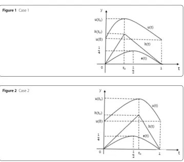
Let
u
take its maximum at
t
0. Then we discuss Lemma
2.6
under the following two
cases.
Case 1.
If 0 <
t
0≤
12, then let
h
(
t
) =
⎧
⎨
⎩
1–t0
t0
t
,
0
≤
t
≤
t
0,
–
t
+ 1,
t
0<
t
≤
1.
Case 2.
If
12
<
t
0< 1, then let
h
(
t
) =
⎧
⎨
⎩
t
,
0
≤
t
≤
t
0,
–
t01–t0
t
+
t0
1–t0
,
t
0<
t
≤
1.
Due to the concavity of
u
and since
h
(
t
0) < 1, we have
u
(
t
)
≥
u
(
t
0)
h
(
t
).
Next we show that
h
(
t
) >
e
(
t
) on
J
holds.
It is easy to see by calculating that
e
(0) = 1,
e
(1) = –1.
On the one hand, when 0 <
t
0≤
12, we have
h
(
t
) =
⎧
⎨
⎩
1–t0
It is obvious that
1 –
t
0t
0> 1,
so by the concavity of
e
we have that
h
(
t
) >
e
(
t
) on
J
.
On the other hand, when
12
<
t
0< 1, we have
h
(
t
) =
⎧
⎨
⎩
1,
0
≤
t
≤
t
0,
–
1–t0t0
,
t
0<
t
≤
1.
It can be easily seen that
–
1 –
t
0t
0< –1,
similarly we can obtain that
h
(
t
) >
e
(
t
) on
J
.
At the same time, by Lemma
2.2
, we have
u
(
t
)
≥
u
(
t
0)
h
(
t
)
≥
u
(
t
0)
e
(
t
)
≥
u
(
t
0)
γ
H
(
t
,
t
) =
bH
(
t
,
t
),
t
∈
J
,
where
b
=
u(γt0).
In order to better understand the above two cases, we draw Figs.
1
and
2
.
This gives the proof of Lemma
2.6
.
Figure 1Case 1
3 Sharp conditions for the existence of positive solutions
In this section, we establish sharp conditions for the existence of positive solutions for
problem (
1.1
) by Lemmas
2.1
–
2.6
. We analyze the following three cases for
ω
∈
L
p[0, 1] :
p
> 1,
p
= 1, and
p
=
∞. Case
p
> 1 is treated in Theorem
3.1
.
Theorem 3.1
Suppose that
(
H
1)
–
(
H
5)
hold
.
Then problem
(
1.1
)
admits a u
∈
C
1[0, 1]
pos-itive solution if and only if
0 <
10
ω
(
s
)
f
(
s
, 1)
ds
< +∞.
Proof
(1) Necessity.
Let
u
∈
C
1[0, 1] be a positive solution of problem (
1.1
), then
u
(0) and
u
(1) exist and are
finite.
On the one hand, we know that
u
(
t
) is a concave function on
J
by
u
≤
0. Therefore,
by Lemma
2.6
, there exists
b
> 0 satisfying
u
(
s
)
≥
bH
(
s
,
s
),
s
∈
J
. Setting
l
=
min
{
b
, 1}, then
u
(
s
)
≥
lH
(
s
,
s
),
s
∈
J
. And by (
1.4
) and Remark
1.2
, we have
10
ω
(
s
)
f
s
,
H
(
s
,
s
)
ds
≤
10
ω
(
s
)
f
s
,
1
l
u
(
s
)
ds
≤ ¯
l
10
–
u
(
s
)
ds
≤ ¯
l
u
(0) –
u
(1)
< +
∞
,
where
¯
l
= (
1l)
λ1.
On the other hand, if we assume that
f
(
s
,
u
(
s
))
≡
0, which shows that
ω
(
s
)
f
(
s
,
u
(
s
))
≡
0
by (
H
1). Then, by Lemma
2.4
, it is obvious that
u
= 0, which contradicts
u
is a positive
solution of problem (
1.1
).
Hence there exists
t
1∈
J
such that
f
(
t
1,
u
(
t
1)) > 0.
And then it follows from (
H
1), Remarks
1.2
and (
1.6
) that
Case 1.
If
ω
(
t
1) > 0, then
0 <
ω
(
t
1)
f
t
1,
u
(
t
1)
≤
ω
(
t
1)
f
t
1,
u
t1≤
ω
(
t
1)
u
t1λ
f
(
t
1
, 1),
where
λ
∈ {
λ
2,
λ
3}.
Case 2.
If
ω
(
t
1) = 0, then it follows from (
H
1) that there exists a small neighborhood
[
a
1,
b
1]
⊂
J
of
t
1such that
ω
(
t
) > 0 for
t
∈
[
a
1,
b
1].
Hence it is easy to see by integration of
f
and
ω
that
b1a1
So,
10
ω
(
s
)
f
(
s
, 1)
ds
≥
10
ω
(
s
)
f
s
,
u
(
s
)
u
ds
≥
1
u
λ∗ 10
ω
(
s
)
f
s
,
u
(
s
)
ds
≥
1
u
λ∗ b1a1
ω
(
s
)
f
s
,
u
(
s
)
ds
> 0,
where
λ
∗∈ {
λ
1,
λ
4}
.
(2) Sufficiency.
(i) First, we prove that the operator
T
:
K
→
K
is completely continuous. For all
u
∈
K
,
T
(
u
)
≥
0 on
J
0, it follows from (
2.18
) and Lemma
2.2
that
(
Tu
)(
t
) =
10
H
(
t
,
s
)
ω
(
s
)
f
s
,
u
(
s
)
ds
≥
θ
10
H
(
t
,
s
)
ω
(
s
)
f
s
,
u
(
s
)
ds
=
θ
Ty
,
∀
t
∈
J
.
So we have that
Tu
∈
K
,
∀
u
∈
K
. Thus
T
(
K
)
⊂
K
.
Next, it follows from Arzelà–Ascoli theorem that
T
:
K
→
K
is completely continuous.
It is clear that
T
is continuous.
Let
B
r=
{
u
∈
E
|
u
≤
r
}
be a bounded set. Then, for all
u
∈
B
r, by the definition of
Tu
and by Lemma
2.2
and Lemma
2.3
, we get
Tu
=
max
t∈J
10
H
(
t
,
s
)
ω
(
s
)
f
s
,
u
(
s
)
ds
≤
γ
10
G
(
s
,
s
)
ω
(
s
)
ds L
≤
γ
G
qω
pL
=
Γ
,
where
L
=
max
t∈J,u∈Brf
(
t
,
u
),
Γ
=
γ
G
qω
pL
.
Therefore, the operator
T
:
K
−→
K
is uniformly bounded.
On the other hand, since
H
(
t
,
s
) is continuous on
J
×
J
, we can see that
H
(
t
,
s
) is
uni-formly continuous on
J
×
J
. Therefore, for any
ε
> 0, there exists
r
> 0, when
|
t
1–
t
2|
<
r
,
we get
H
(
t
1,
s
) –
H
(
t
2,
s
)
<
ε
Accordingly, for all
u
∈
B
r, when
|
t
1–
t
2|
<
r
, we have
(
Tu
)(
t
1) – (
Tu
)(
t
2)
=
10
H
(
t
1,
s
)
ω
(
s
)
f
s
,
u
(
s
)
ds
–
10
H
(
t
2,
s
)
ω
(
s
)
f
s
,
u
(
s
)
ds
=
10
H
(
t
1,
s
) –
H
(
t
2,
s
)
ω
(
s
)
f
s
,
u
(
s
)
ds
≤
ω
1·
L
·
ε
ω
1·
L
≤
ε
.
This shows that the set
{
T
(
u
) :
u
∈
B
r}
is equicontinuous, and it follows from Arzelà–
Ascoli theorem that operator
T
is completely continuous.
(ii) Next, we prove that
T
has at least one fixed point in
K
.
For
u
∈
K
,
u
≤
1, we get
u
(
t
)
≤
u
≤
1, and by (
1.4
) and Remark
1.2
, we obtain
f
t
,
u
(
t
)
≤
u
λ2(
t
)
f
(
t
, 1).
Hence,
Tu
≤
10
γ
G
(
s
,
s
)
ω
(
s
)
u
λ2(
s
)
f
(
s
, 1)
ds
≤
γ
u
λ2G
q
ω
p 10
f
(
s
, 1)
ds
≤
A
u
λ2,
where
A
=
γ
G
qω
p 10
f
(
s
, 1)
ds
.
If (
1A
)
1
λ2–1
≤
1, setting
r
∗ 1= (
A1)
1
λ2–1
, then
Tu
≤
u
,
∀
u
∈
K
,
u
=
r
∗ 1.
If (
A1)
λ2–11> 1, we have
A
< 1. Letting
r
∗∗1
= 1, similarly we have
Tu
≤
u
,
∀
u
∈
K
,
u
=
r
∗∗1.
Set
r
1=
max
{
r
∗1,
r
1∗∗}. Then we obtain
Tu
≤
u
,
∀
u
∈
K
,
u
=
r
1.
Moreover, by Remark
1.2
, there exists
R
>
r
1for
u
≥
R
such that
f
(
t
,
u
(
t
))
u
(
t
)
≥
min
t∈J0f
(
t
,
u
(
t
))
u
(
t
)
≥
N
,
t
∈
J
0,
that is,
f
(
t
,
u
(
t
))
≥
Nu
(
t
),
t
∈
J
0,
u
≥
R
, where
N
> 0 satisfies
N
≥
1
ζ θ
min
t∈J0 1–θθ
H
(
t
,
s
)
ds
.
So, for
u
∈
K
with
u
=
R
, we get
Tu
≥
min
t∈J0
(
Tu
)(
t
)
≥
min
t∈J0
1–θθ
H
(
t
,
s
)
ω
(
s
)
f
s
,
u
(
s
)
ds
≥
min
t∈J0
1–θθ
≥
Nζ
min
t∈J0 θ
H
(
t
,
s
)
u
θ
ds
≥
Nζ θ
min
t∈J0
1–θθ
H
(
t
,
s
)
ds
u
≥
u
.
Thus,
Tu
≥
u
,
∀
u
∈
K
,
u
=
R
.
Lemma
2.5
yields that
T
admits at least one fixed point
u
∗such that
r
1≤
u
∗≤
R
. Since
u
∗(
t
)
≥
u
∗θ
≥
r
1θ
> 0, 0 <
t
< 1, we see that
u
∗is a positive solution of problem (
1.1
).
Moreover, for any
u
∗∈
K
, we have
u
∗(
s
)
≤
u
∗,
s
∈
J
, and then, for
λ
∈ {
λ
2,
λ
3}, we get
10
u
∗(
s
)
ds
=
10
ω
(
s
)
f
s
,
u
∗(
s
)
ds
≤
10
ω
(
s
)
f
s
,
u
∗ds
≤
u
∗λ 10
ω
(
s
)
f
(
s
, 1)
ds
< +
∞
,
that is,
u
∗is absolutely integrable on
J
. This shows that (
u
∗)
(0
+) and (
u
∗)
(1
–) exist, then
u
∗∈
C
1[0, 1]. The proof above shows that
u
∗∈
C
1[0, 1] is a positive solution of (
1.1
). This
completes the proof of Theorem
3.1
.
The following corollary handles the case
p
=
∞
.
Corollary 3.1
Assume that
(
H
1)
–
(
H
5)
hold
.
Then problem
(
1.1
)
admits a u
∈
C
1[0, 1]
pos-itive solution if and only if
0 <
10
ω
(
s
)
f
(
s
, 1)
ds
< +
∞
.
Proof
Let
G
1ω
∞
replace
G
qω
pand repeat the argument of Theorem
3.1
. Then
we can complete the proof of Corollary
3.1
.
At last, we analyze the case of
p
= 1.
Corollary 3.2
Assume that
(
H
1)
–
(
H
5)
hold
.
Then problem
(
1.1
)
has a u
∈
C
1[0, 1]
positive
solution if and only if
0 <
10
ω
(
s
)
f
(
s
, 1)
ds
< +∞.
Proof
Let
14ω
1replace
G
qω
pand repeat the argument of Theorem
3.1
. Then we
can complete the proof of Corollary
3.2
.
Theorem 3.2
Assume f
(
t
,
u
) =
h
1(
t
,
u
) +
h
2(
t
,
u
),
where h
1(
t
,
u
)
and h
2(
t
,
u
)
satisfy
(
H
4),
and the other main hypothesis is also needed
0 <
γ
G
qω
p 10
f
(
s
, 1)
ds
< 1.
Then problem
(
1.1
)
admits at least two C
1[0, 1]
positive solutions if and only if
0 <
10
ω
(
s
)
f
(
s
, 1)
ds
< +∞.
Proof
We first prove that the operator
(
Tu
)(
t
) =
10
H
(
t
,
s
)
ω
(
s
)
f
s
,
u
(
s
)
ds
=
10
H
(
t
,
s
)
ω
(
s
)
h
1s
,
u
(
s
)
+
h
2s
,
u
(
s
)
ds
admits at least two fixed points in
K
.
Choosing
J
1= [
ξ
1,
η
1]
⊂
J
,
τ
1=
min
t∈J1h
1(
t
, 1) and taking a constant
l
> 1 such that
lθ
> 1,
for
u
> 1,
u
∈
K
,
t
∈
J
1, we obtain
lu
(
t
)
≥
lθ
u
>
lθ
> 1,
h
1t
,
u
(
t
)
≥
l
λ2–λ1u
(
t
)
λ2h
1(
t
, 1).
Consequently,
(
Tu
)(
t
)
≥
η1ξ1
H
(
t
,
s
)
ω
(
s
)
h
1s
,
u
(
s
)
+
h
2s
,
u
(
s
)
ds
≥
η1ξ1
G
(
t
,
s
)
ω
(
s
)
h
1s
,
u
(
s
)
+
h
2s
,
u
(
s
)
ds
≥
θ
λ2τ
1
l
(λ2–λ1)ζ
η1ξ1
G
(
ξ
1,
s
)
ds
u
λ2≥
A
u
λ2,
where
A
=
θ
λ2τ
1
l
(λ2–λ1)ζ
η1ξ1
G
(
ξ
1,
s
)
ds
.
Due to
u
> 1,
λ
2> 1, there exists arbitrarily large
R
2> 1 such that
Tu
≥
u
,
∀
u
∈
K
,
u
=
R
2.
When
u
< 1, taking
J
2= [
ξ
2,
η
2]
⊂
J
and
τ
2=
min
t∈J2h
2(
t
, 1), we also get that
(
Tu
)(
t
)
≥
η2ξ2
G
(
t
,
s
)
ω
(
s
)
h
1s
,
u
(
s
)
+
h
2s
,
u
(
s
)
ds
≥
θ
λ4τ
2ζ
η2ξ2
G
(
ξ
2,
s
)
ds
u
λ4≥
A
1u
λ4,
where
A
1=
θ
λ4τ
2ζ
η2Similarly, due to
u
< 1,
λ
4< 1, there exists arbitrarily small
r
2< 1 such that
Tu
≥
u
,
∀
u
∈
K
,
u
=
r
2.
Moreover, because of
u
∈
K
,
u
= 1 and
u
(
t
)
≤
u
= 1
≤
1, we can obtain
h
1t
,
u
(
t
)
+
h
2t
,
u
(
t
)
≤
u
(
t
)
λ2h
1
(
t
, 1) +
u
(
t
)
λ3h
2(
t
, 1)
≤
h
1(
s
, 1) +
h
2(
s
, 1)
.
Accordingly,
(
Tu
)(
t
)
≤
10
γ
G
(
s
,
s
)
ω
(
s
)
h
1s
,
u
(
s
)
+
h
2s
,
u
(
s
)
ds
≤
γ
G
qω
p 10
h
1(
s
, 1) +
h
2(
s
, 1)
ds
< 1 =
u
.
(3.1)
That is,
Tu
<
u
,
∀
u
∈
K
∩
∂Ω
=
{
u
∈
K
:
u
= 1
}
.
Consequently, Lemma
2.5
yields that the operator
T
admits at least two fixed points
u
1(
t
) and
u
2(
t
) in
K
, and
u
1(
t
)
=
u
2(
t
) by (
3.1
).
On the other hand, the proof of necessity is similar to that of Theorem
3.1
, so we omit
it here. The proof of Theorem
3.2
is complete.
4 Remarks and comments
In this section, we provide some remarks and comments related to problem (
1.1
).
Remark
4.1 The proof of Theorems
3.1
–
3.2
is directly inspired by Theorem 1.1 of [
63
],
but there are no papers analyzing sharp conditions of positive solution for second-order
boundary value problems with integral boundary conditions, particularly under the case
ω
is
L
p-integrable.
Remark
4.2 In general, it is difficult to analyze sharp conditions of positive solutions for
nonlinear second-order differential equations (see, e.g., [
1
–
28
] and their references).
Remark
4.3 Similar to the proof of Theorems
3.1
–
3.2
, one can prove sharp conditions of
positive solution for the following problems:
⎧
⎨
⎩
u
(
t
) +
ω
(
t
)
f
(
t
,
u
(
t
)) = 0,
u
(0) =
01g
(
t
)
u
(
t
)
dt
,
u
(1) = 0,
(4.1)
⎧
⎨
⎩
u
(
t
) +
ω
(
t
)
f
(
t
,
u
(
t
)) = 0,
u
(0) = 0,
u
(1) =
01g
(
t
)
u
(
t
)
dt
,
(4.2)
Acknowledgements
We wish to express our thanks to Prof. Meiqiang Feng, School of Applied Science, Beijing Information Science & Technology University, Beijing, PR China, for his kind help, careful reading, and making useful comments on the earlier version of this paper. The authors are also grateful to anonymous referees for their constructive comments and suggestions which have greatly improved this paper.
Funding
This work is sponsored by the National Natural Science Foundation of China (11301178) and the Beijing Natural Science Foundation of China (1163007).
Availability of data and materials
Not applicable.
Ethics approval and consent to participate
Not applicable.
Competing interests
The authors declare that there is no conflict of interests regarding the publication of this manuscript. The authors declare that they have no competing interests.
Consent for publication
Not applicable.
Authors’ contributions
The authors contributed equally in this article. They have all read and approved the final manuscript.
Publisher’s Note
Springer Nature remains neutral with regard to jurisdictional claims in published maps and institutional affiliations.
Received: 27 March 2019 Accepted: 21 October 2019
References
1. Hao, X., Zuo, M., Liu, L.: Multiple positive solutions for a system of impulsive integral boundary value problems with sign-changing nonlinearities. Appl. Math. Lett.82, 24–31 (2018)
2. Mao, J., Zhao, Z.: The existence and uniqueness of positive solutions for integral boundary value problems. Bull. Malays. Math. Sci. Soc.34, 153–164 (2011)
3. Jiao, L., Zhang, X.: A class of second-order nonlocal indefinite impulsive differential systems. Bound. Value Probl.2018, 163 (2018)
4. Zhang, X.: Exact interval of parameter and two infinite families of positive solutions for anth order impulsive singular equation. J. Comput. Appl. Math.330, 896–908 (2018)
5. Hao, X., Liu, L., Wu, Y.: Positive solutions for second order impulsive differential equations with integral boundary conditions. Commun. Nonlinear Sci. Numer. Simul.16, 101–111 (2011)
6. Wang, Y., Liu, L., Zhang, X., Wu, Y.: Positive solutions of an abstract fractional semipositone differential system model for bioprocesses of HIV infection. Appl. Math. Comput.258, 312–324 (2015)
7. Autuori, G., Cluni, F., Gusella, V., Pucci, P.: Mathematical models for nonlocal elastic composite materials. Adv. Nonlinear Anal.6, 355–382 (2017)
8. Zhang, X., Ge, W.: Symmetric positive solutions of boundary value problems with integral boundary conditions. Appl. Math. Comput.219, 3553–3564 (2012)
9. Hao, X., Liu, L., Wu, Y.: Positive solutions for singular second order differential equations with integral boundary conditions. Math. Comput. Model.57, 836–847 (2013)
10. Hao, X., Liu, L., Wu, Y., Sun, Q.: Positive solutions for nonlinearnth-order singular eigenvalue problem with nonlocal conditions. Nonlinear Anal., Theory Methods Appl.73, 1653–1662 (2010)
11. Hao, X., Wang, H., Liu, L., Cui, Y.: Positive solutions for a system of nonlinear fractional nonlocal boundary value problems with parameters andp-Laplacian operator. Bound. Value Probl.2017, 182 (2017)
12. Zhang, X., Feng, M.: Existence of a positive solution for one-dimensional singularp-Laplacian problems and its parameter dependence. J. Math. Anal. Appl.413, 566–582 (2014)
13. Hao, X., Xu, N., Liu, L.: Existence and uniqueness of positive solutions for fourth-orderm-point boundary value problems with two parameters. Rocky Mt. J. Math.43, 1161–1180 (2013)
14. Hao, X., Liu, L., Wu, Y.: On positive solutions of anm-point nonhomogeneous singular boundary value problem. Nonlinear Anal., Theory Methods Appl.73, 2532–2540 (2010)
15. Zhang, X., Feng, M.: Double bifurcation diagrams and four positive solutions of nonlinear boundary value problems via time maps. Commun. Pure Appl. Anal.17, 2149–2171 (2018)
16. Zhang, X., Liu, L., Wu, Y.: The uniqueness of positive solution for a fractional order model of turbulent flow in a porous medium. Appl. Math. Lett.37, 26–33 (2014)
17. Zhong, Q., Zhang, X.: Positive solution for higher-order singular infinite-point fractional differential equation with p-Laplacian. Adv. Differ. Equ.2016, 11 (2016)
18. Dong, X., Bai, Z., Zhang, S.: Positive solutions to boundary value problems ofp-Laplacian with fractional derivative. Bound. Value Probl.2017, 5 (2017)
20. Wu, J., Zhang, X., Liu, L., Wu, Y., Cui, Y.: Convergence analysis of iterative scheme and error estimation of positive solution for a fractional differential equation. Math. Model. Anal.23, 611–626 (2018)
21. He, J., Zhang, X., Liu, L., Wu, Y., Cui, Y.: Existence and asymptotic analysis of positive solutions for a singular fractional differential equation with nonlocal boundary conditions. Bound. Value Probl.2018, 189 (2018)
22. Zhang, X., Mao, C., Liu, L., Wu, Y.: Exact iterative solution for an abstract fractional dynamic system model for bioprocess. Qual. Theory Dyn. Syst.16, 205–222 (2017)
23. Zhang, X., Zhong, Q.: Triple positive solutions for nonlocal fractional differential equations with singularities both on time and space variables. Appl. Math. Lett.80, 12–19 (2018)
24. Hao, X., Zhang, L., Liu, L.: Positive solutions of higher order fractional integral boundary value problem with a parameter. Nonlinear Anal., Model. Control24, 210–223 (2019)
25. Hao, X., Wang, H.: Positive solutions of semipositone singular fractional differential systems with a parameter and integral boundary conditions. Open Math.16, 581–596 (2018)
26. Mao, J., Zhao, Z., Wang, C.: The exact iterative solution of fractional differential equation with nonlocal boundary value conditions. J. Funct. Spaces2018, Article ID 8346398 (2018)
27. Guan, Y., Zhao, Z., Lin, X.: On the existence of positive solutions and negative solutions of singular fractional differential equations via global bifurcation techniques. Bound. Value Probl.2016, 141 (2016)
28. Feng, M., Li, P., Sun, S.: Symmetric positive solutions for fourth-ordern-dimensionalm-Laplace systems. Bound. Value Probl.2018, 63 (2018)
29. Cannon, J.R.: The solution of the heat equation subject to the specification of energy. Q. Appl. Math.21, 155–160 (1963)
30. Chegis, R.Yu.: Numerical solution of a heat conduction problem with an integral boundary condition. Liet. Mat. Rink.
24, 209–215 (1984)
31. Qin, P., Feng, M., Li, P.: Positive solutions to one-dimensional quasilinear impulsive indefinite boundary value problems. Adv. Differ. Equ.2018, 421 (2018)
32. Jiang, J., Liu, L., Wu, Y.: Positive solutions for second order impulsive differential equations with Stieltjes integral boundary conditions. Adv. Differ. Equ.2012, 124 (2012)
33. Zhang, X., Feng, M., Ge, W.: Existence result of second-order differential equations with integral boundary conditions at resonance. J. Math. Anal. Appl.353, 311–319 (2009)
34. Zhang, X., Ge, W.: Symmetric positive solutions of boundary value problems with integral boundary conditions. Appl. Math. Comput.219, 3553–3564 (2012)
35. Guo, L., Liu, L., Wu, Y.: Iterative unique positive solutions for singularp-Laplacian fractional differential equation system with several parameters. Nonlinear Anal., Model. Control22, 182–203 (2018)
36. Zhang, X., Liu, L., Wu, Y., Wiwatanapataphee, B.: The spectral analysis for a singular fractional differential equation with a signed measure. Appl. Math. Comput.257, 252–263 (2015)
37. Zhang, X., Liu, L., Wu, Y.: Variational structure and multiple solutions for a fractional advection-dispersion equation. Comput. Math. Appl.68, 1794–1805 (2014)
38. Zhang, X., Liu, L., Wu, Y.: The uniqueness of positive solution for a fractional order model of turbulent flow in a porous medium. Appl. Math. Lett.37, 26–33 (2014)
39. Kong, L.: Second order singular boundary value problems with integral boundary conditions. Nonlinear Anal., Theory Methods Appl.72, 2628–2638 (2010)
40. Wei, Y., Bai, Z., Sun, S.: On positive solutions for some second-order three-point boundary value problems with convection term. J. Inequal. Appl.2019, 72 (2019)
41. Jiang, J., Liu, L., Wu, Y.: Second-order nonlinear singular Sturm–Liouville problems with integral boundary problems. Appl. Math. Comput.215, 1573–1582 (2009)
42. Zhang, X., Liu, L., Wiwatanapataphee, B., Wu, Y.: The eigenvalue for a class of singularp-Laplacian fractional differential equations involving the Riemann–Stieltjes integral boundary condition. Appl. Math. Comput.235, 412–422 (2014) 43. Li, P., Feng, M., Qin, P.: A class of nonlocal indefinite differential systems. Bound. Value Probl.2018, 81 (2018) 44. Boucherif, A.: Second-order boundary value problems with integral boundary conditions. Nonlinear Anal., Theory
Methods Appl.70, 364–371 (2009)
45. Feng, M.: Existence of symmetric positive solutions for a boundary value problem with integral boundary conditions. Appl. Math. Lett.24, 1419–1427 (2011)
46. Yan, F., Zuo, F., Hao, X.: Positive solution for a fractional singular boundary value problem withp-Laplacian operator. Bound. Value Probl.2018, 51 (2018)
47. Karakostas, G.L., Tsamatos, P.Ch.: Multiple positive solutions of some Fredholm integral equations arisen from nonlocal boundary-value problems. Electron. J. Differ. Equ.2002, 30 (2002)
48. Zhang, X., Liu, L., Wu, Y.: The eigenvalue problem for a singular higher fractional differential equation involving fractional derivatives. Appl. Math. Comput.218, 8526–8536 (2012)
49. Feng, M., Ge, W.: Positive solutions for a class ofm-point singular boundary value problems. Math. Comput. Model.
46, 375–383 (2007)
50. Jiang, J., Liu, L., Wu, Y.: Positive solutions forp-Laplacian fourth-order differential system with integral boundary conditions. Discrete Dyn. Nat. Soc.2012, Article ID 293734 (2012)
51. Lan, K.: Multiple positive solutions of semilinear differential equations with singularities. J. Lond. Math. Soc.63, 690–704 (2001)
52. Zhang, X., Liu, L., Wu, Y.: Existence results for multiple positive solutions of nonlinear higher order perturbed fractional differential equations with derivatives. Appl. Math. Comput.219, 1420–1433 (2012)
53. Guo, L., Liu, L., Wu, Y.: Existence of positive solutions for singular fractional differential equations with infinite-point boundary conditions. Nonlinear Anal., Model. Control21, 635–650 (2016)
54. Zhang, X., Liu, L., Wu, Y., Lu, Y.: The iterative solutions of nonlinear fractional differential equations. Appl. Math. Comput.219, 4680–4691 (2013)
55. Zhang, X., Liu, L., Wu, Y., Wiwatanapataphee, B.: Nontrivial solutions for a fractional advection dispersion equation in anomalous diffusion. Appl. Math. Lett.66, 1–8 (2017)
57. Li, P., Feng, M.: Denumerably many positive solutions for an-dimensional higher-order singular fractional differential system. Adv. Differ. Equ.2018, 145 (2018)
58. Ahmad, B., Alsaedi, A.: Existence of approximate solutions of the forced Duffing equation with discontinuous type integral boundary conditions. Nonlinear Anal., Real World Appl.10, 358–367 (2009)
59. Sun, F., Liu, L., Zhang, X., Wu, Y.: Spectral analysis for a singular differential system with integral boundary conditions. Mediterr. J. Math.13, 4763–4782 (2016)
60. Liu, L., Sun, F., Zhang, X., Wu, Y.: Bifurcation analysis for a singular differential system with two parameters via to topological degree theory. Nonlinear Anal., Model. Control22, 31–50 (2017)
61. Zhang, X., Liu, L., Wu, Y.: Multiple positive solutions of a singular fractional differential equation with negatively perturbed term. Math. Comput. Model.55, 1263–1274 (2012)
62. Zhang, Y.: Positive solutions of singular sublinear Emden–Fowler boundary value problems. J. Math. Anal. Appl.185, 215–222 (1994)
63. Zhao, Z.: A necessary and sufficient condition for singular nonlinear second-order boundary value problems to have positive solutions. Annal. Math. JCU13B, 15–24 (1998)
64. Zhang, X., Tian, Y.: Sharp conditions for the existence of positive solutions for a second-order singular impulsive differential equation. Appl. Anal., 1–13 (2017)
65. Yang, F.: Necessary and sufficient conditions for existence of positive solutions to a class of singular second order boundary value problems. Chin. J. Eng. Math.25, 281–287 (2008)
66. Pouso, R.: Necessary and sufficient conditions for existence and uniqueness of solutions of second-order autonomous differential equations. J. Lond. Math. Soc.2, 397–414 (2005)
67. Du, X., Zhao, Z.: A necessary and sufficient condition for the existence of positive solutions to singular sublinear three-point boundary value problems. Appl. Math. Comput.186, 404–413 (2007)
68. Cid, J., Pouso, R., Enguiça, R.: Sharp conditions for the existence of solutions of second-order autonomous differential equations. Mediterr. J. Math.42, 191–214 (2007)
69. Zhao, J., Wang, L., Ge, W.: Necessary and sufficient conditions for the existence of positive solutions of fourth order multi-point boundary value problems. Nonlinear Anal.72, 822–835 (2010)
70. Zhang, X., Feng, M.: The existence and asymptotic behavior of boundary blow-up solutions to thek-Hessian equation. J. Differ. Equ.267, 4626–4672 (2019)
71. Zhang, X., Du, Y.: Sharp conditions for the existence of boundary blow-up solutions to the Monge–Ampère equation. Calc. Var. Partial Differ. Equ.57, 30 (2018)
72. Zhang, X., Feng, M.: Boundary blow-up solutions to thek-Hessian equation with a weakly superlinear nonlinearity. J. Math. Anal. Appl.464, 456–472 (2018)
73. Feng, M., Zhang, X.: On ak-Hessian equation with a weakly superlinear nonlinearity and singular weights. Nonlinear Anal.190, 111601 (2020)
74. Zhang, X., Feng, M.: Boundary blow-up solutions to the Monge–Ampère equation: sharp conditions and asymptotic behavior. Adv. Nonlinear Anal.9, 729–744 (2020)
75. Feng, M., Zhang, X.: On ak-Hessian equation with a weakly superlinear nonlinearity and singular weights. Nonlinear Anal.190, 111601 (2020)
76. Guo, D., Lakshmikantham, V.: Nonlinear Problems in Abstract Cones. Academic Press, New York (1988)