Modeling and Optimization of Turning Duplex Stainless Steels

Stainless Steels

Von der Fakultät Konstruktions-, Produktions- und Fahrzeugtechnik der Universität Stuttgart zur Erlangung der

Würde eines Doktors der Ingenieurwissenschaften (Dr.-Ing.) genehmigte Abhandlung

Vorgelegt von

M. Sc. Rastee Dalshad Ali (Koyee) aus Erbil, Kurdistan-Irak

Hauptberichter: Univ.-Prof. Dr.-Ing. Prof. h. c. mult. Dr. h. c. mult. Uwe Heisel i. R. Mitberichter: Prof. Dr. rer. nat. Siegfried Schmauder

Tag der mündlichen Prüfung: 14.04.2015

Vorwort

Hiermit möchte ich all denen meinen Dank aussprechen, die mich bei der Entstehung dieser Arbeit unterstützt und zu ihrem Gelingen beigetragen haben. In diesem Zusammenhang sei dem Deutsche Akedemische Austauschdienst für die finanzielle Unterstützung und Förderung gedankt.

Dem Leiter des Institutes, Univ.-Prof. Dr.-Ing. Prof. h. c. mult. Dr. h. c. mult. Uwe Heisel i. R. gilt mein besonderer Dank für die Möglichkeit zur Durchführung der Arbeit und den dafür notwendigen Freiraum ebenso wie für die Übernahme des Hauptberichtes und die dabei ent-standenen Anregungen.

Herrn Prof. Dr. rer. nat. Siegfried Schmauder danke ich sehr herzlich für die teilweise Betreu-ung meiner Arbeit. Seine freundliche UnterstützBetreu-ung meiner wissenschaftlichen Tätigkeit, sei-ne ständige Bereitschaft zu fachlichen Diskussiosei-nen mit vielen wertvollen Ratschlägen und konstruktiven Anregungen haben maßgeblich zur Realisierung dieser Arbeit beigetragen. Herrn Dipl.-Ing Dipl.-Gwl. Rocco Eisseler, meinem langjährigem Kollege und Gruppenleiter, danke ich für zahlreiche konstruktive fachliche Diskussionen, die ebenso wie seine Tipps zu formalen Aspekten der schriftlichen Ausarbeitung eine wertvolle Hilfe geleistet haben.

Ein herzlicher Dank gebührt weiterhin meinen Kollegen und Freunden, durch die ich meine Promotionszeit in schöner Erinnerung behalten werde. Frau Inge Özdemir, Herrn Dr.-Ing. Michael Schaal, Herrn Dipl.-Ing. Atanas Mishev, Herrn Dipl.-Ing. (FH) Jens Großmann, Herrn Rolf Bauer und Herrn Dr.-Ing. Johannes Rothmund vielen Dank für Ihre Freundschaft und Hilfsbereitschaft.

Mein ganz besonderer Dank gilt letztlich meinem Vater Dalshad sowie meinen Geschwistern, Dipl. Rasper, Dipl.-Ing. Rawand, Dr. Rawa, Dipl.-Ing. Rawen und B.Sc. Suham, und meinen Cousinen Dr. Narmin Koye, Dr. Bahzad Koye und Dr. Kurdo Koye für ihre fortwährende liebevolle Unterstützung. Ihr Verständnis, ihre oft endlose Geduld sowie ihre unermüdliche moralische Aufbauarbeit haben mir den notwendigen familiären Rückhalt zur Durchführung dieser Arbeit gegeben.

Für die Seele meiner Mutter

Ehrenwörtliche Erklärung

Hiermit erkläre ich, dass ich die vorliegende Arbeit selbstständig verfasst und keine anderen als die angegebenen Hilfsmittel genutzt habe. Alle wörtlich oder inhaltlich übernommenen Stellen habe ich als solche gekennzeichnet. Ich versichere außerdem, dass ich die vorliegende Arbeit keiner anderen Prüfungsbehörde vorgelegt habe und, dass die Arbeit bisher auch auf keine andere Weise veröffentlicht wurde. Ich bin mir der moralischen und gesetzlichen Kon-sequenzen einer falschen Aussage bewusst.

Legal statement

I solemnly declare that I have produced this work all by myself. Ideas taken directly or indi-rectly from other sources are marked as such. This work has not been shown to any other board of examiners so far and has not been published yet. I am fully aware of moral and legal consequences of making a false declaration.

Contents

Nomenclature X 

Extended Abstract XIX 

1  Einleitung XIX 

2  Forschungsmethodik XX 

2.1  Hypothesen XXI 

2.2  Gliederung der Dissertation XXI 

2.3  Die Vorgehensweisen XXII 

3  Zusammenfassung XXIX 

Summary XXXI 

1  Introduction 1 

1.1  Frame of reference 4 

1.1.1  Metal cutting 5 

1.2  Background and aim 24 

1.3  Research approach 25 

1.4  Research hypothesis 26 

1.5  Research questions 27 

1.6  Research delimitations 28 

1.7  Outline of the dissertation 28 

2  State of the art in machining modeling and optimization: A review 32  2.1  Input-output parameter relationship of modeling tools 33 

2.1.1  Statistical regression 34 

2.1.2  Neural network 39 

2.1.3  Fuzzy set theory 43 

2.2  Finite element modeling of chip formation processes 47  2.2.1  Basics of FEM formulations and remeshing techniques 49 

2.2.3  Scales of the machining modeling 52  2.2.4  Simulation software & phases of metal cutting FEA 53  2.2.5  Advantages and problems associated with numerical cutting modeling 54  2.2.6  Input models and identification of input parameters 56  2.3  Determination of optimal or near-optimal cutting conditions 62 

2.3.1  Taguchi Method 63 

2.3.2  Response surface methodology (RSM) 68 

2.3.3  Nature-inspired meta-heuristic algorithms 73 

2.3.4  Multiple Attribute Decision Making (MADM) methods 86  2.4  A systematic methodology for modeling and optimization of cutting processes 102 

3  Experimental details 106 

3.1  Workpiece materials 106 

3.1.1  Mechanical properties and chemical compositions 106  3.1.2  Temperature-dependent physical and mechanical properties of the workpiece materials 107 

3.2  Machine tool and cutting tool 110 

3.3  Design of experiments (DOE) 112 

3.3.1  Full factorial design 112 

3.3.2  Taguchi designs 113 

3.3.3  D-Optimal design 115 

3.4  Measurement of the machining performance characteristics 116  3.4.1  Measurement of cutting forces and effective cutting power 116  3.4.3  Measurement of surface quality characteristics 117 

3.4.4  Measurement of the flank wear 118 

3.4.5  Infrared temperature measurement system 120 

3.4.6  Chip thickness and chip serration ratio 121 

4  Experimental investigation and multi-objective optimization of turning DSSs: A case

study 122 

4.2  Performance characteristics 123 

4.2.1  Specific cutting pressures 123 

4.2.2  The width of maximum flank wear land (VB_max) 125  4.3  Bat Algorithm for multi-objective optimization of turning DSSs. 130 

4.4  Interim conclusions 132 

5  Universal Characteristics Index 134 

5.1  Estimation of the chip volume ratio 135 

5.2  Universal characteristics index 137 

5.2.1  TOPSIS 138 

5.2.2  VIKOR method 139 

5.2.3  GRA 139 

5.2.4  UC 139 

5.2.5  Fuzzy-MADM 140 

5.3  Optimization 142 

5.4  Interim conclusions 145 

6  Taguchi-MADM-Meta-heuristic concept 146 

6.1  Taguchi method 146 

6.2  VIKOR method 150 

6.3  Meta-heuristic optimization 152 

6.4  Interim conclusions 155 

7  Application of Fuzzy–MADM approach in optimizing surface quality of stainless

steels 157 

7.1  Proposed methodology 157 

7.2  Results and discussions 160 

7.2.1  Computation of the MSQCIs 160 

7.2.2  Fuzzy-MADM method 162 

7.3  Confirmation tests 166 

8  Sustainability-based multi-pass optimization of cutting DSSs 169 

8.1  Performance characteristics 170 

8.2  Phase I: Parametric cutting investigations 172 

8.2.1  Effect of control factors on performance characteristics 173  8.2.2  Parametric optimization of performance characteristics 178 

8.3  Phase II: Economics of cutting DSSs 180 

8.4  Phase III: Operational sustainability index 182 

8.4.1  Optimization of OSI using CSNNS 185 

8.5  Interim conclusions 189 

9  Numerical modeling and optimization of turning DSSs 193 

9.1  3D FEM prediction of the chip serration 194 

9.2  3D FEM prediction of the chip serration 198 

9.3  Inverse identification of 3D FEM input parameters 202 

9.3.1  Proposed methodology 207 

9.3.2  Extension of FANNS: a case study 215 

9.4  Inverse identification of Usui’s wear model constants 215 

9.5  Numerical optimization of turning DSSs 217 

9.5.1  Selective control factors 218 

9.5.2  Results and discussions 220 

9.5.3  Numerical machining performance measure 227 

9.6  Interim conclusions 230 

10 Conclusions 233 

11 References 238 

Nomenclature

List of Latin symbols:

Symbol Unit Definition

A MPa Initial yield strength



A Negative ideal solution

*

A Positive ideal solution

a

A €/(m2_{.Month) Monthly rent} c

A mm2 _{Cutting area}

l

A Loudness

p

a mm Depth of cut

b Bias

B Strain hardening coefficient

C Strain rate coefficient

*

C Closeness to the ideal solution

CB Chip-breaker type

f

C A constant function of cutting length

CI Consistency Index

CM Cooling medium

n

c Coefficient of regression equations

p

C J/kg. K _{Heat capacity}

CR Consistency Ratio

2

%C Percentage of ON state of the machine

d mm Outside diameter

D MPa Cockcroft-Latham material constant

. crit

D MPa _{Critical damage value}

DV Degree of diversification

e Error terms in regression and neural network analyses

E J Energy

c

Symbol Unit Definition

c

E €/kWh _{Electricity cost}

j

E Entropy of attribute j

E

% Percentage error

c

F N _{Main cutting force}

f

F N _{Feed cutting force}

q

f Frequency

r

f mm/rev Feed rate

t

F N _{Thrust cutting force}

t F

% Percentage increase in thrust cutting force *

g Global best

.

Geo Insert shape

GRG Grey relational grade

H Chip serration ratio

h mm Chip thickness

tc

h N/(mm.sec.K) Thermal contact conductance

I Intensity of light of a firefly

c

I A _{Line current}

JAS hrs Annual operating hours

k Order of neural network layers

1

K € _{Main time-related costs}

1 . 1

k MPa _{Specific cutting pressure for 1mm}2 _{cutting area} 2

K € _{Fixed or the workpiece-related costs}

3

K € _{Tool-related costs}

b

k m2 _kg/(sec2 _{K) Boltzmann constant} bB

k € _{Procurement cost}

bE

k € _{Operational cost}

bR

k € _{Space cost}

bW

Symbol Unit Definition

c

k MPa _{Specific cutting pressure}

ET

k € _{Cost of the spare parts}

f

k MPa _{Specific feed pressure}

F

K € Total production cost

k

k €/hrs _{Coolant cost}

L

K € Labor cost

M

K € Machine hour-rate cost

ML

K € Machine and wage rate cost

n

K Number of control factors

r

K degree Cutting edge anle

KT µm Depth of the crater wear

t

k MPa _{Specific thrust pressure}

th

k W/(m2.K) _{Thermal conductivity} WH

k € _{Cost of the tool holder}

WP

k € _{Cost of the cutting insert}

L Number of levels

c

L mm _{Length of cut}

m

L €/hrs _{Hourly wage of labor}

r

l mm _{Approach length}

s

L mm _{Sample length}

t

L mm _{Travel length}

m units Number of the production units

m Thermal softening exponent in JC model

MRR mm3/min Material removal rate

N rpm Rotational speed

p

n _{Number of cutting passes}

t

N Number of experimental trials

Symbol Unit Definition

a

P Probability

c

P W _{Cutting power}

e

P W _{Effective pwer}

M

P W Motor power

PN Preference number

r

P Pulse emission

sp

P W _{Net spindle power}

p p

% Percentage of the procurement cost

r p

% Percentage decrease in flow stress

m

Q m2 _{Machine-tool basement area}

NN

Q VIKOR index predicted by neural networks

V

Q VIKOR index

i q

% Percentage of the interest rate

R Chip volume ratio

r € Amount of non-wage costs of the machine operator 2

R Coefficient of determination

Ra µm Arithmetic average roughness

adj.

R Adjusted coefficient of determination

c

R N _{Resultant cutting force}

RI Random Index

i

R Regret measure

Rt µm Highest roughness point from the mean

Rz µm Average absolute value of five peaks and valleys 

r mm _{Nose radius}

R~ Centroid



S Negative ideal alternative

*

S Positive ideal alternative

i

S Utility measure

Symbol Unit Definition

a

t hrs _{Working time}

bB

t hrs _{Machine utilization time}

c

t min _{Cutting time}

e

t min _{Production time or time per unit} g

t min _{Basic time}

h

t min _{Main process time}

i

t min _{Idle time}

l

t years _{Economic machine life}

m

T °C _{Melting temperature}

r

T °C _{Reference temperature}

n

t min _{Auxiliary process time} q

t Target of the neural network

rB

t min set-up time

rV

t min _{Nonproductive set-up activities time} rW

t min _{Tool change time}

vM

t min _{Machine set-up time}

WZ

t min _{Time that passes till a single tool is changed} c

U Utility constant

l

U V _{Line voltage}

V Mean square of neural network error

VB µm Average width of the flank wear land max

VB µm _{Maximum width of the flank wear land}

n

VB µm _{Average width of the notch wear land} c

v m/min Cutting speed

s

v m/sec _{Sliding velocity}

w Weight of the attributes

W µm Wear

Symbol Unit Definition *

x Individual best

s

Z Number of cutting edges per insert

List of Greek symbols:

Symbol Unit Definition

n

 degree Normal rake angle

rand

 Randomization parameter

z

 Step size scaling factor in Cuckoo Search algorithm a

 Firefly attractiveness

r

 Random vector drawn from a uniform distribution

w

 degree Wedge angle

r

 Euclidean distance between fireflies

 Deviation squence

c

 degree _{Chip flow angle}

 Equivalent plastic strain

 Equivalent plastic strain rate

0

 sec-1 Reference plastic strain rate f

 Effective strain

p

 _{Von Mises equivalent plastic strain}

 N/(mm.sec) Heat flux

 J Conducted heat

n

 degree _{Normal shear angle}

s

 degree _{Shear angle}

p

 W/m3 _{Volumetric heat generation} a

 Randomization parameter in Firefly Algorithm

c

 degree Relief or clearance angle

 dB Signal to Noise ratio

t

 Taylor-Quinney coefficient

 Expectation of occurrence

Symbol Unit Definition

i

 degree _{Inclination angle}

w

 Wavelength in Bat Algorithm

 _{Friction coefficient}

A

 Membership function of set A

c

 Coulomb friction coefficient

s

 Shear friction coefficient

T

 °C _{Mean tool face temperature}

m

 kg/m3 _Density

 _{Degree of uncertainty}

1

 MPa Principal stress

n

 MPa _{Normal stress}

 MPa Von Mises equivalent stress

 _{Learning parameter}

f

 MPa _{Frictional stress}

 Random number drawn from a uniform distribution

 Acceleration constant

 Weight of the strategy

 _{Activation function of neurons}

g

 Random number drawn from Gaussian distribution

 Learning rate

g

 Grey relational coefficient

List of abbreviations:

Abbreviation Description

AAD Absolute Average Deviation

AHP Analytical Hierarchy Process

ALE Arbitrary Lagrangian-Eulerian

ANN Artificial Neural Networks ANOM Analysis of Means

ANOVA Analysis of Variance

Abbreviation Description

BUE Built-up edge

CS Cuckoo Search

CSNNS Cuckoo Search Neural Network Systems

CV Crisp Value

DC Discontinuous Chips

DOE Design of Experiment DOF Degree of Freedom DSS Duplex Stainless Steel

FA Firefly Algorithm

FANNS Firefly Algorithm Neural Network System FEM Finite Element Method

FIS Fuzzy Inference System GRA Grey Relational Analysis

GTMA Graph Theory and Matrix Approach JMatPro Java-based Material Properties

LB Lower Bound

LCFC Long Cylindrical and Flat helical Chips LHCS Long Helical Chip Segments

LM Lower Medium

LRSC Long Ribbon and Snarled Chips

LSC Long Spiral Chips

MADM Multiple Attribute Decision Making

MH Moderately High

ML Moderately Low

MLP Multi-Layer Perceptron

MOBA Multi-Objective Bat Algorithm

MOO Multi-Objective Optimization

MPCI Multi-Performance Characteristics Index MSE Mean Square Error

MSQCI Multi-Surface Quality Characteristics Index

OA Orthogonal Array

OSI Operational Sustainability Index

Abbreviation Description

RMSE Root Mean Square Errors RSM Response Surface Methodology

SA Simulated Annealing

SCFC Short Cylindrical and Flat helical Chips SHCS Short Helical Chip Segments

SRSC Short Ribbon and Snarled Chips

SS Sum of Squares

SSC Short Spiral Chips

STDV Standard Deviation

TOPSIS Technique for Order Preference by Similarity to Ideal Solution

UB Upper Bound

UC Utility Concept

UCI Universal Characteristics Index

UM Upper Medium

VH Very High

Extended Abstract

1 Einleitung

Der Mensch nutzt seit rund 5000 Jahren das Metall Eisen. Aber erst im 18. Jahrhundert stoßen Wissenschaftler in kurzer Folge auf eine ganze Reihe zuvor unbekannter Metalle. Im Jahr 1751 entdeckte z.B. der schwedische Wissenschaftler Axel Cronstedt das Element Nickel. 1778 folgte sein Landsmann Karl Wilhelm Scheele mit dem Element Molybdän. 1797 fand der Franzose Nicola-Louis Vauquelin ein neues Metall, das er Chrom nannte. Im 19. Jahrhun-dert experimentierten mehrere Metallurgen erfolgreich mit Eisen-Chrom Legierungen. Zwar zeigt sich, dass sie besonderes rostbeständig sind, allerdings waren die Gründe hierfür noch nicht bekannt.

1912 wurde den beiden Deutschen Edward Maurer und Beno Strauß ein Patent auf austeneti-sche Chrom-Nickel-Stähle erteilt. Noch heute machen die austenitiausteneti-schen Sorten rund 65% der Weltproduktion an rostfreiem Stahl aus. 1913 wurde in England erstmals martensitischer rost-freier Stahl hergestellt. Der Entdecker dieser Neuerung war Harry Brearley. Ungefähr zur selben Zeit, nämlich 1915, entwickelten die US-Amerikaner Becket und Dantsaizen ferriti-sche rostfreie Stähle. Auf sie entfallen 30% der weltweiten Erzeugung. Bis 1920, also in we-niger als einem Jahrzehnt, bildete sich auf diese Weise der hauptsächliche Anwendungsgebie-te.

1930 entwickelten schwedische Metallurgen Stahlsorten, die sowohl ein ferritisches als auch ein austenitisches Gefüge in einer Legierung vereinen, und bezeichneten diese als rostfreie Duplexstähle. Duplexstähle revolutionierten zunächst die Zellstoff- und Papierindustrie durch die Verfügbarkeit beständiger Bauteile. Heute bewähren sie sich in einer ganzen Reihe von Anwendungen, z.B. in der petrochemischen Industrie oder bei der Meerwasser-Entsalzung, also dort wo sowohl eine besondere Korrosionsbeständigkeit als auch eine hohe Festigkeit erforderlich sind.

Seit 1990 findet eine zweite Generation von rostfreien Duplexstähle immer mehr breiteren Einsatz als Alternative zu den konventionellen rostfreien Stählen. Die Gründe hierfür sind:

3. Deutlich höhere Korrosionsbeständigkeit gegen durch Chlorid induzierte Spannungs-korrosion als dies bei austenitischen rostfreien Stählen der Fall ist.

Andererseits sind die rostfreien Duplexstähle normalerweise schwerer zerspanbar als austeni-tische Sorten mit einer vergleichbaren Korrosionsbeständigkeit. Die Gründe sind: große Zä-higkeit, niedrige WärmeleitfäZä-higkeit, hohe Streckgrenzwerte (ca. zweimal höher als austeniti-sche rostfreie Stähle), spezielle Mikrostruktur (weiches Ferrit neben hartem Austenit), gerin-ger Schwefel- und Phosphorgehalt, starke Tendenz zu Bildung von Aufbauschneiden und eine hohe Kaltverfestigungsrate.

Aufgrund der hohen Zähigkeit bilden sich oftmals beim Zerspanen lange Band- oder Wirr-späne aus, die sich um das Werkstück oder den Werkzeughalter wickeln können. Die Proble-matik verschärfte sich besonders bei Schlichtoperationen mit geringen Vorschüben und Schnitttiefen. In der automatisierten Fertigung verringert dies die Produktivität aufgrund von Maschinenstillstandszeiten sowie geringer Prozesssicherheit in erheblichem Maße.

2 Forschungsmethodik

rechnerischer Modellierungs- sowie Optimierungsverfahren dar. Diese werden im Rahmen der Ansätze zur Zerspanungsoptimierung effektiv angewendet.

2.1 Hypothesen

Ausgehend von der Frage, wie die Verwendung von neu entwickelten Modellierungs- und Optimierungsverfahren für eine effektive Ableitung von optimierten Zerspanungslösungen ermöglicht werden kann, werden systematische Untersuchungen unter Einsatz von neuentwi-ckelten Modellierungs- und Optimierungsverfahren durchgeführt. Zunächst sollen jedoch die folgenden Hypothesen vorgestellt werden:

1. Statistische Regression und metaheuristische Optimierungsverfahren können zu einer Reihe von nicht dominanten Zerspanungslösungen führen.

2. Fuzzylogik ist vorteilhaft zur Beseitigung der Diskrepanz in der Rangordnung von Alter-nativen unter dem Einsatz von MKES.

3. Das Taguchi-MKES-metaheuristisches Konzept kann praktischerweise für Mono- und Mehrzieloptimierungen verwendet werden.

4. Merkmale der Oberflächenqualität können effizient optimiert werden, wenn MKES mit der Fuzzy-Set-Theorie gekoppelt werden.

5. Die Multipass-Zerspanung kann nachhaltig optimiert werden, wenn eine systematische Hybridisierung des Modells der Ein- und Ausgangkenngrößen sowie der Optimierung und der MKES durchgeführt wird.

6. Es ist ausreichend, die JMatPro Software, MKES und Modelle sowie Optimierungsansät-ze für Ein- und Ausgangkenngrößen zur Rückwärtsidentifikation von FEM-Eingangskenngrößen zu benutzen.

2.2 Gliederung der Dissertation

Kapitel 4 befasst sich mit experimentellen Untersuchungen zum Längsdrehen von rostfreien Duplexstählen mit beschichteten Wendeschneidplatten. In Kapitel 5 wird die Beseitigung von Diskrepanzen bei der MKES-Rangordnung durch die Ableitung eines allgemeinen Eigen-schafts-Zeiger-Index behandelt. In Kapitel 6 wird die Anwendung eines neuen Taguchi-VIKOR- metaheuristischen Konzepts als angemessener Ansatz für die Mono- und Mehrzielo-ptimierung der Bearbeitung von rostfreien Duplexstählen aufgeführt. In Kapitel 7 wird die Taguchi-Methode in Verbindung mit der Fuzzy-MKES für die Optimierung von Merkmalen der Oberflächengüte angewandt. In Kapitel 8 wird ein systematischer Ansatz vorgelegt, der unterschiedliche Modellierungs- und Optimierungsverfahren integriert, um die Multipass-Zerspanung von rostfreien Duplexstählen nachhaltig zu optimieren. Kapitel 9 befasst sich mit der Rückwärtsidentifikation der FEM-Eingangskenngrößen und der Anwendung der Finite-Elemente-Simulationen, um damit eine hypothetische Optimierungsstudie durchzuführen. In Kapitel 10 werden die Forschungsfragen, welche der vorliegenden Arbeit zugrunde lagen, beantwortet und abschließenden besprochen.

2.3 Die Vorgehensweisen

2.3.1 Die Fledermaus-Mehrzieloptimierung

Im Zusammenhang mit der Haupthypothese stellt sich die erste Forschungsfrage wie folgt: Kann durch die Anwendung der statistischen Regression und des Metaheuristischen Optimie-rungsverfahren in Mehrzieloptimierungen eine Reihe von nichtdominierten Zerspanungslö-sungen effektiv gewonnen werden? Um diese Frage angemessen zu beantworten, wird eine experimentelle Untersuchung des Längsdrehens von rostfreien Duplexstählen EN 1.4462 und EN 1.4410 mit beschichteten Wendelschneidplatten durchgeführt. Mit Hilfe des Fledermaus-Mehrziel-Algorithmus (MOBA) werden Bewertungskriterien wie beispielsweise die Zerspan-kraftkomponenten und die maximale Verschleißmarkenbreite optimiert und die Pareto Gren-zen der nicht dominierten Optimierungslösungen ermittelt. Die parametrischen Einflüsse von Größen wie Schnittgeschwindigkeit, Vorschub und Kühlmedium auf die Bewertungskriterien werden mit Hilfe von dreidimensionalen Diagrammen dargestellt.

Steigerung der Werkzeugstandzeit. Drittens wird nach der Regressionsanalyse ein MOBA zur Modellierung eingesetzt. Ergebnisse zeigen, dass der MOBA sehr effizient und sehr zuverläs-sig ist. Er führt effizient zu vielen optimalen Lösungen. Abhängig vom Entscheidungsträger-vorzug wird die optimale Schnittbedingung identifiziert.

2.3.2 Der allgemeine Eigenschaftenzeiger

Die zweite Forschungsfrage lautet: Ist die Anwendung von Fuzzylogik vorteilhaft zur Besei-tigung von Widersprüchlichkeiten in der Rangordnung beim Einsatz von MKES? Als bei-spielhafter Zerspanungsprozess wird hierzu das Plandrehen bei konstanter Schnittgeschwin-digkeit herangezogen. Das Plandrehen zeichnet sich im Vergleich zum Außenlängsdrehen durch eine bessere Wirtschaftlichkeit, höhere Oberflächengüte und kürzere Hauptzeit aus. Leistungsmerkmale wie Spanraumzahl, resultierende Schnittkraft, spezifische Schnittkraft und Netto-Spindelleistung sollen gleichzeitig optimiert werden.

Unter den vielen maßgeblichen Leistungsmerkmalen ist die Spanraumzahl eine der wichtigs-ten. Die Spanraumzahl gibt Auskunft über die Sperrigkeit der Späne. Sie wird aus dem Ver-hältnis von Spänevolumen zu Spanungsvolumen gebildet. Allerdings ist die messtechnische Erfassung des Spänevolumens in der Praxis nicht einfach. Um dieses zumindest hinreichend abschätzen zu können, wird deshalb eine neue Methode vorgeschlagen. Zunächst werden qua-litative Informationen über die Späne in einer Spanbruchtabelle dargestellt. Anschließend werden die Späne gemäß den bekannten Standardspanformen klassifiziert. Dann kommt die Fuzzylogik zum Einsatz, wobei Regeln formuliert werden, um die qualitativen Informationen zu fuzzifizieren. Abschließend werden die fuzzifizierten Daten im Fuzzy-Inferenz-System zu quantitativen Daten defuzzifiziert und zur Vorhersage der Spanrauzahl genutzt.

Die unterschiedlichen Leistungsmerkmale werden zudem mit Hilfe von MKES wie TOPSIS, VIKOR, GRA und UA in einem einzelnen MKES-Index zusammengeführt. Basierend auf einer unterschiedlichen MKES-Präferenz und der Tatsache, dass keine MKES als optimales Verfahren anzusehen ist, wird schließlich die Mamdani-Fuzzy-Begründung genutzt, um den Widerspruch zwischen den MKES aufzulösen und einen allgemeinen Index abzuleiten. Dieser Index wird als allgemeiner Eigenschaftenzeiger (UCI) bezeichnet. Der optimierte UCI wird anhand der Ergebnisse von zwei weiteren Optimierungsverfahren validiert.

Bei diesen Verfahren handelt es sich um:

2. Statistische Regression ergänzt durch eine simulierte Abkühlung.

Die Ergebnisse zeigen, dass mit diesem Ansatz die aus anderen anderen Optimierungsverfah-ren resultieOptimierungsverfah-rende, durchschnittliche Verbesserung der Leistungsmerkmale übertroffen werden kann. Im Allgemeinen sind durchschnittliche Verbesserungen zwischen 10% und 40% mög-lich.

Aus diesen Ergebnissen kann geschlossen werden, dass der neue Ansatz wirkungsvoller ist, als die anderen klassischen Ansätze.

2.3.3 Das Taguchi-VIKOR-metaheuristische Konzept

Kann das Taguchi-VIKOR-metaheuristische Konzept praktischerweise für Monoziel- und Mehrzieloptimierungen der Zerspanung von rostfreien Stählen verwendet werden? Dies ist die dritte Frage in der Folge des Erkenntnisgewinns. Zunächst werden hierzu die Schnittbe-dingungen als Einflussgrößen und das Plandrehen mit konstanter Schnittgeschwindigkeit als Zerspanprozess festgelegt.

Anschließend wurden Zerspanversuche gemäß der Taguchi-Methode durchgeführt. Bei der Taguchi-Methode werden im Wesentlichen orthogonale Felder eingesetzt. Orthogonale Felder sind Teilfaktorpläne, d.h. es werden nicht alle möglichen Kombinationen von Faktorstufen durchgespielt, sondern nur eine genau ausgewählte Teilmenge. Durch diesen Ansatz kann man die Zahl der erforderlichen Experimente erheblich reduzieren. Im konkreten Fall müssen so anstelle von 125 Experimenten nur 25 Experimente durchgeführt werden. Die Leistungs-merkmale, die gleichzeitig optimiert werden sollen, sind die Schnittleistung, die resultieren-den Schnittkräfte, die spezifische Schnittenergie und der arithmetische Mittenrauwert. Die Vorgehensweise ist wie folgt:

Im zweiten Schritt wird die Mehrzieloptimierung durchgeführt und hierzu die VIKOR-Methode eingesetzt. VIKOR gehört zu einer Kompromissklassifizierung der MKES. Sie be-ginnt mit einer Datennormalisierung auf Werte zwischen 0 und 1. Anschließend werden die Gewichte der einzelnen Leistungsmerkmale mit Hilfe der Entropiegewichtsmethode berech-net. Anschließend erfolgt die statistische Kalkulation der Utility, Regret und des VIKOR-Index und der entsprechenden Rangordnung der Alternativen. Man kann diesen VIKOR-Index auch als Schwerzerspanbarkeitsindex bezeichnen. Je kleiner der Wert des VIKOR-Index desto bes-ser. Es handelt sich um einen Index, der genau darauf hinweist, wo sich der optimale Schnitt-parameterbereich befindet.

Der dritte Schritt, um die wirkungsvollsten metaheuristischen Optimierungsverfahren zu er-mitteln und die exakten Schnittbedingungen zu bestimmen, besteht darin, drei neuentwickelte, metaheuristische Algorithmen anzuwenden und ihre Leistung zu verglichen. Die betrachteten drei neuentwickelten, metaheuristischen Optimierungsverfahren sind der Glühwürmchen-Algorithmus, die beschleunigte Partikel-Schwarm-Optimierung und der Kuckuck-Suchalgorithmus. Diese Algorithmen wurden entsprechend der gegebenen Entscheidungsva-riablen, Zielfunktionen und Zwänge eingesetzt. Die Ergebnisse zeigten, dass der Kuckuck-Suchalgorithmus die anderen Optimierungsalgorithmen übertrifft.

Zusammenfassen wird bewiesen, dass das Taguchi-VIKOR-metaheuristische Konzept prakti-scherweise für Monoziel- und Mehrzieloptimierung der Zerspanung rostfreier Stähle verwen-det werden kann.

2.3.4 Die Optimierung von Merkmalen der Oberflächengüte

Die vierte Frage befasst sich mit der Optimierung von Merkmalen der Oberflächengüte. Unter Zuhilfenahme von MKES und Fuzzy-Set-Theorie werden die Größen zur Bewertung der Oberflächengüte namentlich der arithmetische Mittenrauwert, die gemittelte Rautiefe und die maximale Rautiefe parallel optimiert. Zu diesem Zweck wird ein neuer Ansatz dargestellt. Der Zerspanungsprozess wird wiederum das Plandrehen mit konstanter Schnittgeschwindig-keit und als Eingangsgrößen die Schnittbedingungen festgelegt. Taguchi-Versuchspläne wer-den verwendet, um wer-den gesamten Hauptparameterraum mit einer geringen Anzahl von Versu-chen abarbeiten zu können.

Festle-gung der Leistungsmerkmale. Im zweiten Schritt werden MKES, wie GTMA und AHP-TOPSIS benutzt, um einen allgemeinen Index für die Merkmale der Oberflächengüte zu be-stimmen. Es stellt sich die Frage, warum hier zwei MKES genutzt werden: Es gibt kein MKES als globales Verfahren, das für alle Arten von Mehrzieloptimierungsproblemen geeig-net ist. Aus diesem Grund ist der Entscheidungsablauf immer mit Unsicherheiten behaftet. Um dieses Problem zu lösen, wird im zweiten Schritt die Fuzzy-Set-Theorie herangezogen. Alle Merkmale der Oberflächengüte müssen in Fuzzy-Trapenznummern überführt werden und unter Einhaltung von 10%-Unsicherheit im Entscheidungsablauf konvertieren. Dann wird die Methode der Gewichteten Summen zur Ableitung von Kompromisslösungen verwendet und die geometrischen Eigenschaften der Trapenznummern werden zur Defuzzifizierung der Indizes genutzt. Schließlich werden die defuzzifizierten Zahlen nachbearbeitet. Die Nachbe-arbeitung befasst sich mit der Anwendung der Mittelwert- und Varianzanalyse sowie der Ve-rifikation der optimierten Ergebnisse.

Nach der Anwendung und Verifikation des Ansatzes, wird die erreichte Verbesserung der Merkmale der Oberflächengüte ermittelt. Hier zeigt sich, dass Verbesserungen von bis zu 30% bei der Oberflächengüte möglich sind. Deshalb kann zusammenfasst werden, dass die beschriebene Vorgehensweise zielführend ist.

2.3.5 Die nachhaltige Optimierung der Multipass-Zerspanung

Im Zusammenhang mit den Hypothesen stellt sich die fünfte Frage: ist es möglich, durch eine systematische Hybridisierung des Modells und der Optimierung der Ein- und Ausgangkenn-größen und durch die MKES die Multipass-Zerspanung nachhaltig zu optimieren?

Stu-fenabstände wesentlich größer, als die Nachteile, wie beispielsweise zu wenig Versuchspunk-te in der MitVersuchspunk-te des Versuchsraumes und die Abhängigkeit von Rechenalgorithmen.

Die Steuerungsfaktoren sind hier numerisch und kategorisch. Erstmalig werden Leistungs-merkmale, wie die prozentuale Erhöhung der radialen Schnittkraft, die Spanraumzahl, die Wirkleistung und die maximale Verschleißmarkenbreite, in der Zerspanungsoptimierung der rostfreien Duplexstähle genutzt.

Die Vorgehensweise des Studiums vollzieht sich systematisch in drei Phasen. In Phase 1 wer-den mathematische Modelle für die Leistungsmerkmale mit der Response-Surface-Methode (RSM) entwickelt, die Wechselwirkungseffekte zwischen Schnittbedingungen und Leis-tungsmerkmalen mit Hilfe von dreidimensionalen Diagrammen analysiert und eine parametri-sche Optimierung der Leistungsmerkmale unter Verwendung des Kuckuck-Suchalgorithmus durchführt. In der Phase 2 werden umfassende Modelle zur Kalkulation von Produktionskos-ten und ProduktionsraProduktionskos-ten entwickelt. Um den Konflikt zwischen dem Wunsch nach minimier-ten Produktionskosminimier-ten und maximierter Produktionsrate überwinden zu können, wird TOPSIS als Optimierungsansatz vorgeschlagen. Die Betriebsmittel-belegungszeit, die Hauptzeitkosten, die Werkzeug- und Werkzeugwechselkosten werden für die Herstellung einer Zahl von 12.000 Stück optimiert und hieraus die beste Alternativ identifiziert. Ein Ansatz zur Modellie-rung und OptimieModellie-rung eines Betriebsnachhaltigkeitsindexes (BNI) wird in der dritten Phase der Vorgehensweise präsentiert. Zuerst wird durch die Anwendung der Mamdani-Implikation ein neuer Index für die nachhaltige Mehrschnitt-Zerspanung von rostfreien Stählen abgeleitet. Durch das BNI kann genau bestimmt werden, wo der Bereich nachhaltiger Zerspanungspara-meter liegt. Der nächste Schritt beinhaltet die Modellierung und Optimierung. Ein neues Ver-fahren nutzt ein künstliches neuronales Netz mit integriertem Kuckuck-Suchalgorithmus (CSNNS). Das BNI kann gleichzeitig und effizient durch den entwickelten CSNNS modelliert und optimiert werden.

Schließlich kann festgehalten werden, dass die systematische Hybridisierung des Modells und der Optimierung der Ein- und Ausgangkenngrößen sowie die MKES Methoden die Zer-spanung der rostfreien Duplexstähle nachhaltig optimieren können.

2.3.6 Die Rückwärtsidentifikation der FEM-Eingangskenngrößen

Vorteil, Eingangskenngrößen wie die Thermokontakt-Leifähigkeit, den Coulombschen Reib-koeffizienten, den Schub-ReibReib-koeffizienten, den Taylor-Quinney-Koeffizienten, die Festig-keitsabnahme und das Cockcroft-Latham-Schadenskriterium und deren Wechselwirkung mit den gegebenen Schnittbedingungen zu kennen.

Bevor die FEM-Simulation erstellt wird, werden die mechanischen und physikalischen Eigen-schaften der Werkstoffe als Funktion der Temperatur ermittelt. Zu diesem Zweck wurde JMatPro eine Java-basierte Software zur Herleitung von Materialeigenschaften genutzt. Phy-sikalische Eigenschaften, wie die Wärmleitfähigkeit, der thermische Ausdehnungs-koeffizient und die spezifische Wärmekapazität, werden als Funktionen der Temperatur dargestellt. Auch wurden die mechanischen Eigenschaften, wie Fließkurven, Elastizitätsmodul und Poissonzahl als Funktion der Temperatur ausgedrückt. Aus diesen wichtigen Informationen wird zunächst ein Textfile erzeugt, um dieses dann in die Keyword-Datei der aktuellen Simulation kopieren zu können.

Um die Eignung von JMatPro für Bereitstellung von Daten für Zerspanungssimulationen zu bewerten, wurde die FE-Simulation unter ähnlichen Eingangsgrößen mit dem Cook-Model verglichen. Die Ergebnisse zeigen, dass die JMatPro-basierte Simulation die Johnson-Cook Simulation übertrifft, besonders wenn die Späne-Morphologie als Bewertungskriterium herangezogen wird.

Zur Rückwärtsidentifikation von FEM-Eingangskenngrößen wird ein L18 -Taguchi-Versuchsplan verwendet. Nach den experimentellen Untersuchungen und Simulationsrech-nungen werden für beide Fälle die prozentualen Fehler zwischen Schnittkraft, Temperatur an der Werkzeugspitze und Spandicke gerechnet und als Leistungsmerkmale definiert. Dann wird die VIKOR-Methode verwendet, um alle prozentualen Fehleranteile zu einem Index zu konvertieren. Dieser Index ist eine Funktion der Eingangsgrößen und wird mit dem neuent-wickelten FANNS (Firefly Algorithm Neural Network System) optimiert. Am Ende dieser Phase werden die Ergebnisse validiert.

Es kann deshalb gesagt werden, dass die vorgeschlagene Vorgehensweise die Eingangskenn-größen sehr effektiv identifiziert und die Fehleranteile der FEM-Rechnung zehn bis zwanzig-fach reduziert.

2.3.7 Hypothetische FEM-Optimierung

In der zweiten Phase der FEM-Studie wird eine neue Vorgehensweise zur FEM-basierten Optimierung beschrieben. Einflussgrößen wie Spänebrecher, die Form der Wendeschneidplat-te, das Kühlschmiermedium, die Schnittgrößen und Neigungswinkel werden durch den inten-siven Einsatz von Taguchi-Optimierungsmethoden und Fuzzylogik optimiert. Die Bewer-tungskriterien sind in diesem Fall resultierende Schnittkraft, Spannung, Schnitttemperatur und Verschleißrate. Eine neue Maßnahme wird von diesen Merkmalen abgeleitet. Es werden 81 Regeln je Werkstoff formuliert und in das Mamdani-Fuzzy-Inferenz-System integriert. Die Ausgabe der Defuzzifizierung wird als numerischer Zerspanungsleistungsindex (NZLI) be-zeichnet.

Nach der Durchführung der FEM-Simulationen und Ableitung des NZLI, wird eine Mittel-wertanalyse des NZLI durchgeführt. Je größer der Wert des NZLI ist, desto besser. Abschlie-ßend zeigen die Ergebnisse, dass die Vorgehensweise für die weitere Entwicklung und Ver-besserung des Zerspanungsprozesses verwenden werden kann.

3 Zusammenfassung

Summary

The global production of stainless steel nearly doubles every ten years and a high growth rate, which has exceeded that of other metals and alloys, indicate the importance of such alloy classes. While there is no controversy over the significant contribution of stainless steels to the well-being of humanity, there is still a lot of room for research works intended to optimize the application of alloys to the manufacturing processes. Owing to the importance of machin-ing as one of the most important classes of manufacturmachin-ing processes, the cuttmachin-ing of stainless steels attracted a lot of attention long ago. However, there still remain some families of alloys of which their machining has not been thoroughly investigated yet. Belonging to the family of alloys and combining properties such as high strength, high corrosion resistance and a rela-tively low price of modern duplex stainless steels have made the material an attractive alterna-tive to the more widely used family of austenitic stainless steels. In spite of the importance and popularity potential, investigations on the machining of modern duplex stainless steels have attracted little attention until very recently.

On the other hand, with the onset of more and more powerful computers and superior soft-ware, enthusiasm for computer modeling and the optimization of machining processes has continued to grow. The interest in computer modeling and optimization is justified by the fact that perceptive achievement of the optimal process performance is rarely possible, even for a highly skilled operator. Moreover, the large number of variables as well as the complex and stochastic nature of the machining process make the decision-making process more difficult. Therefore, an alternative approach is frequently used to identify the relationship between the performance characteristics of the process and the control factors via mathematical models and/or to represent the dynamics of the system via simulation, after the performance of the process has been optimized using a suitable optimization algorithm.

1 Introduction

There is no doubt that stainless steels are an important class of alloys. Their importance is manifested in the plenitude of applications that rely on their use. From low-end applications, like cooking utensils and furniture, to very sophisticated ones, such as space vehicles, the use of stainless steels is indispensable. In fact, the omnipresence of stainless steels in our daily life makes it impossible to enumerate their applications [Lula86]. The importance of stainless steels may be more appreciated by looking at the compound annual growth rate of the world stainless steel production in the last six decades as shown in Figure 1.1.

Figure 1.1: Compound annual growth rate of world stainless melt shop production (slab/ingot equivalent): 1950 – 2013 in Mt [Issf13].

Figure 1.2: Comparison of the per-capita consumption of stainless steel in selected countries [Rasc12].

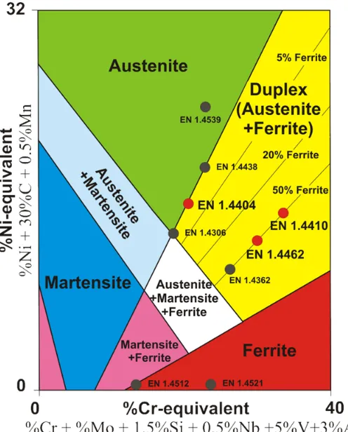
aluminum and titanium. They attain higher strength, toughness and corrosion resistance than strictly martensitic stainless steels [Bram01].

Figure 1.4: Classification chart for stainless steels.

1.1 Frame

of

reference

Machining is a general term describing a group of manufacturing processes that consist of the removal of material and the modification of the surfaces of a workpiece after it has been pro-duced by various methods [KaSc08]. The importance of machining can be econimcally envis-aged. In the US, for instance, industries spend annually well over $100 billion to perform metal removal operations because the vast majority of manufactured products require machin-ing at some stage in their production, rangmachin-ing from relatively rough or nonprecision work, such as cleanup of castings or forgings, to high-precision work, involving tolerances of 0.0025mm or less and high-quality finishes. Thus machining is undoubtedly the most im-portant of the basic manufacturing processes [BlKo13].

can be compared in terms of the value of tool life, cutting power, surface finish, dimensional accuracy, chip control and part cost under similar cutting conditions. Other criteria can also be employed, for example, cutting temperature, operator safety, etc., see Figure 1.5 [KaSc08].

Figure 1.5: Traditionally used machinability assessment criteria [Jawa88].

There are seven traditional machining processes: turning, milling, drilling, sawing, broaching, shaping (planing), and grinding (also called abrasive machining). As an introduction to the field, the following section is intended to describe the fundamentals of metal cutting processes with particular focus on turning processes and the factors influencing the machinability of metals during turning processes.

1.1.1 Metal cutting

Figure 1.6: Fundamental input and outputs of the metal cutting process.

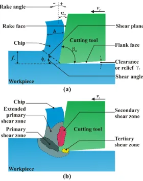
Figure 1.7: Schematic illustration of two-dimensional cutting processes: (a) orthogonal cut-ting with a well-defined shear plane (b) orthogonal cutcut-ting without a well-defined shear plane. Chip formation in metal cutting is a complex chemical-physical process accompanied by large plastic deformation of the workpiece material and very high strain rates. Basically, there are three deformation zones in the cutting process as shown in the cross-sectional view of the orthogonal cutting (see Figure 1.7 (b)). As the edge of the tool penetrates into the workpiece, the material ahead of the tool is sheared over the primary shear zone to form a chip. The sheared material, i.e., the chip, is partially deformed and moves along the rake face of the tool, which is called secondary deformation zone. The friction area where the flank of the tool rubs the newly machined surface is called tertiary zone [AlBe12, PHLT08].

present, as well as chip curl and depicts tool face friction as being elastic rather than plastic. In 1966, Zorev [Zore63] proposed a ‘fan’-type or pie-shaped shear zone model through re-placing curvilinear boundaries by straight lines. Later, Oxley [Oxle89] developed a model with parallel-sided shear bands inclined at a certain angle to the tool motion boundaries [Grze09].

The majority of machining operations involve tool shapes that are three-dimensional, thus the cutting is oblique. The mechanics of complex, three-dimensional oblique cutting operations are usually evaluated by geometrical and kinematic transformation models applied to the or-thogonal cutting process. A simplified schematic representation of the oblique cutting process is shown in Figure 1.8.

The process is performed by tools with a tool cutting edge angle of Kr ≠ 90° and a tool incli-nation angle of λi ≠ 0°. The rake angle may be measured in more than one plane, and hence more than one rake angle can be defined for a given tool and angle of obliquity. The different rake angles in oblique cutting are called normal (αn), velocity and effective rake angle. The flow of chip is at an angle to the normal to the cutting edge. The angle between normal to the cutting edge and chip velocity vector is called chip flow angle (Δc). The shear angles can also be measured in different planes such as a plane normal to the cutting edge (ϕn) and plane of effective rake angle [AlBe12, BlKo13, Grze09, KaSc08].

1.1.1.1 Surface roughness

Roughness refers to the small, finely spaced deviations from the nominal surface that are de-termined by the material characteristics and the process that formed the surface [Groo10]. It is one of the most important measurable quality characteristics and one of the most frequent customer requirements. Surface roughness greatly affects the functional performance of me-chanical parts, such as wear resistance, fatigue strength, ability of distributing and holding lubricant, heat generation and transmission, corrosion resistance, etc.

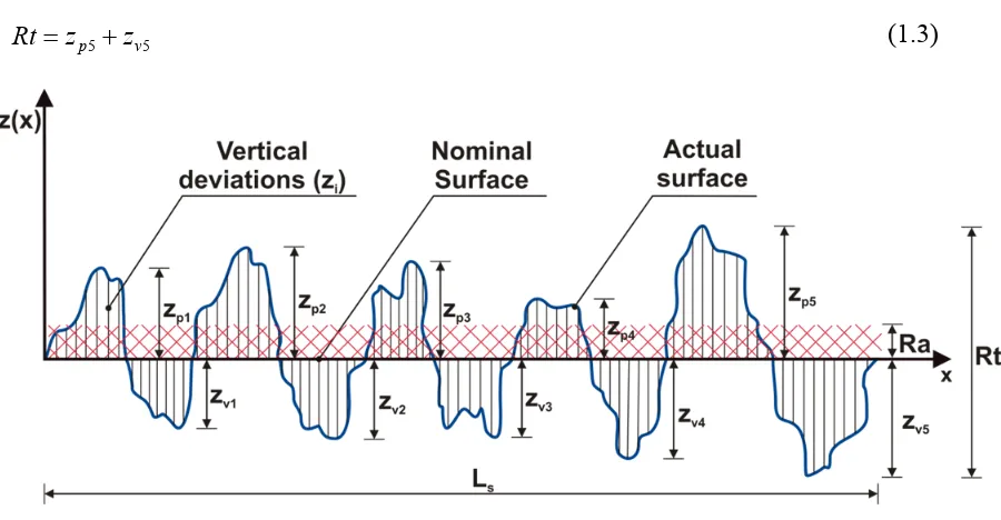
JIS 1994 has defined six parameters in roughness profiles. The reader should refer to the standard for complete definitions of each parameter [SeCh06]. However, since the ranges of definition seem to be dictated by the physical possibilities of existing measuring instruments, it can be assumed that the definitions can also be extended to values below those, but this must be investigated.

 Ra is the most widely used quantification parameter in surface texture measurement. In the past, it was also known as center line average (CLA) or in the USA as arithmetic aver-age (AA). Ra is the arithmetic average value of the profile departure from the mean line within a sampling length, which can be defined as:





 n

i i L

s

z n dx x z L Ra

s

1 0

1 )

(

1 (1.1)

where L_sis the sample length, and zis the height from the mean line defined in Figure 1.9.  Rz is the sum of the average absolute value of the height of the five highest peaks as

measured from the average line and the average absolute value of the height of the five lowest valleys within a portion stretching over a sample length (Ls) in the direction in which the average line extends.





 



 5

1 5

1 5

1 5

1

i v

i pi i

z z

Rz (1.2)

where z_piand z_viare the highest peaks and deepest valleys respectively.

5 5 v p z z

Rt  (1.3)

Figure 1.9: Definition of the surface roughness parameters.

1.1.1.2 Energy and power in turning

Turning is a process of removing excess material from the workpiece to produce an axisym-metric surface, in which the workpiece rotates in a spindle and the tool moves in a plane per-pendicular to the surface velocity of the workpiece at the tool-workpiece contact point [DiDi08]. Based on the direction of the feed motion, one can differentiate between longitudi-nal turning, facing and form turning. In the first case there is an axial feed, in the second case a radial feed and in the third case a simultaneous axial and radial feed motion [Chry06]. The first case is used to produce cylindrical surfaces, the second is utilized to produce flat surfaces at the end of the part and perpendicular to its axis, and the third is used to produce various axisymmetric shapes for functional or aesthetic purposes [KaSc06].

 F_c: Main cutting force acting in the direction of the cutting velocity vector. This force is generally the largest force and accounts for 99% of the power required by the process.  F_f : Feed force acting in the direction of the tool feed. This force is usually about 50% of

c

F but accounts for only a small percentage of the power required because feed rates are usually small compared with cutting speeds.

 F_t: Thrust or radial force acting perpendicular to the machined surface. This force is typi-cally about 50% of Ff and contributes very little to power requirements because velocity in the radial direction is negligible.

The resultant cutting force (R_c) and the power required for cutting (P_c) can be calculated from the following equations:

2 2 2

t f c

c F F F

R    (1.4)

c c c Fv

P  (1.5)

Figure 1.10: (a) Longitudinal turning and (b) facing operations have three measurable compo-nents of forces acting on the tool. These forces vary with cutting speed (v_c), feed rate ( f_r)

and depth of cut (ap).

generally known as the specific (volumetric) cutting energy (ec) and both quantities are equiv-alent to the specific cutting pressure (k_c).

c c c c p r c c c c k F v a f v F MRR P e      (1.6)

where _cis cross-sectional area of the uncut chip. Similarly, the values of the specific cutting pressures related to the feed forces k_f and thrust forces k_t can be evaluated using the expres-sions: c f f F k   (1.7) c t t F k   (1.8)

The value of the cutting force can also be predicted using the modified Kienzle equation:

 

r a

c _f

v k

F  

      1 1 . 1 100 (1.9)

whereF represents the described cutting and resultant forces, k_1.1 is the specific cutting pres-sure for a 1mm2 cross-sectional area of the cut, and the exponents a and b are model con-stants [BlKo13, Grze09, Kloc11].

1.1.1.3 Tool wear

During metal cutting, cutting tools are subjected to:  high localized stresses at the tip of the tool,  high temperatures, especially along the rake face,  sliding of the chip along the rake face, and

 sliding of the tool along the newly cut workpiece surface.

Wear is a gradual process, much like the wear of the tip of an ordinary pencil. The rate of tool wear depends on tool and workpiece materials, tool geometry, process parameters, and the characteristics of the machine tool. Tool wear and the changes in tool geometry during cutting manifest themselves in different ways, generally classified as flank wear, crater wear, nose wear, notching, plastic deformation of the tool tip, chipping, and gross fracture [KaSc06]. Figure 1.11 shows wear forms that occur primarily on turning tools [Kloc11].

Figure 1.11: Characteristic wear forms at the cutting part during the turning process. Figure 1.12 is a schematic representation of the dimensions of wear. In particular, we distin-guish the width of flank wear land VB, the displacement of cutting edge toward flank face SVα and rake face SVγ , the crater depth KT and the crater center distance KM, from which

the crater ratio K = KT/KM is formed.

The mechanisms that cause wear at the tool–chip and tool–work interfaces in machining can be summarized as follows:

 Adhesion. When two metals are forced into contact under high pressure and temperature, adhesion or welding occur between them. These conditions are present between the chip and the rake face of the tool. As the chip flows across the tool, small particles of the tool are broken away from the surface, resulting in attrition of the surface.

Figure 1.12: Wear forms and measured quantities at the cutting part, according to the DIN ISO 3685 [Kloc11].

 Diffusion. This is a process in which an exchange of atoms takes place across a close con-tact boundary between two materials. In the case of tool wear, diffusion occurs at the tool– chip boundary, causing the tool surface to become depleted of the atoms responsible for its hardness. As this process continues, the tool surface becomes more susceptible to abra-sion and adheabra-sion. Diffuabra-sion is believed to be a principal mechanism of crater wear.  Chemical reactions. The high temperatures and clean surfaces at the tool–chip interface in

machining at high speeds can result in chemical reactions, in particular, oxidation, on the rake face of the tool. The oxidized layer, being softer than the parent tool material, is sheared away, exposing new material to sustain the reaction process.

tempera-ture cause the edge to deform plastically, making it more vulnerable to abrasion of the tool surface. Plastic deformation contributes mainly to flank wear.

Most of these tool-wear mechanisms are accelerated at higher cutting speeds and tempera-tures. From those, diffusion and chemical reaction are especially sensitive to elevated tem-peratures [Groo10].

1.1.1.4 Chip morphologies in turning

A chip is enormously variable in shape and size in industrial machining operations. The for-mation of all types of chips involves a shearing of the work material in the region of a plane extending from the tool edge to the position where the upper surface of the chip leaves the work surface. Gray cast iron chips, for example, are always fragmented, and the chips of more ductile materials may be produced as segments, particularly at very low cutting speeds. This discontinuous chip is one of the principal classes of chip forms and has the practical ad-vantage that it is easily cleared from the cutting area. Under the majority of cutting conditions, however, ductile metals and alloys do not fracture on the shear plane, and a continuous chip is produced. Continuous chips may adopt many shapes - straight, tangled or with different types of helix. Often they have considerable strength, and the control of the chip shape is one of the problems confronting machinists and tool designers. Continuous and discontinuous chips are not two sharply defined categories; every shade of gradation between the two types can be observed. Another category of chips is observed when layers of workpiece material are grad-ually deposited on the tool tip, forming the built-up edge (BUE). As it grows larger, the BUE becomes unstable and eventually breaks apart. Part of the BUE material is carried away by the tool side of the chips; the rest is randomly deposited on the workpiece surface. The cycle of BUE formation and destruction is repeated continuously during the cutting operation until corrective measures are taken [KaSc06, TrWr00].

curve #2). When the entire shear strain decreases further, the chip segmentation starts to de-velop and the separation of chip segments begins (elemental chips vs. #3). In this case, the material necking takes place before the fracture but at a relatively lower shear stress. It should be noted that all three types of chips formed by shearing mechanisms could generally be relat-ed to the plastic deformation of the ductile work materials. In contrast, brittle materials only undergo elastic deformation (curve #4), which leads to producing discontinuous chips [Grze09].

Figure 1.13: (a) Chip formation in terms of stress-strain curves according to Weber and Loladze; and (b) Fridman diagram of the fracture mechanism [Grze08].

per-fectly ductile material (c). Additionally, line a’ represents some specific case when the shear stress is artificially lowered due to intensive cooling by supplying gaseous or liquid coolants. Inclined lines starting from the origin of such a coordinate system represent simple tension (1), simple compression (2) and simple torsion (3). Consequently, three types of material frac-ture can be distinguished, namely: brittle fracfrac-ture in point A, partially ductile fracfrac-ture in point C because of the linear work-hardening effect and perfect ductile fracture in point E. It can be assumed that these mechanical material states are equivalent to those responsible for the for-mation of discontinuous, segmented and continuous types [Grze08].

1.1.1.5 Chip volume ratio (R)

With regard to the metal removal rate, one has to distinguish between the volume of the re-moved material MRR and the space needed for the randomly arranged metal chips. The vol-ume of the removed material identifies the volvol-ume occupied by a chip with cross sectional areaΑ_c. The volume of the randomly arranged metal chips removed is greater than the real volume of the same amount of removed material, since in a reservoir the chips are not located next to each other without gaps. The chip volume ratio R defines by what factor the volume of randomly arranged chips is greater than the volume of the removed material.

removal metal

of amount same

the of volume Material

chips metal arranged randomly

for needed Volume



R (1.10)

Figure 1.14 summarizes the most significant chip shapes. Each chip form is assigned to a chip volume ratio R, which defines by what factor the transport volume needed for the specific chip form exceeds the intrinsic material volume of the chip.

Figure 1.14: Chip shapes and chip volume ratios [BBCC09].

1.1.1.6 Economics of turning operations

The economics of machining has been an important area of research in machining starting with the early work of Gilbert [Gilb50]. The main objectives are the minimization of the ma-chining cost, the maximization of the production rate and the maximization of the profit rate. The major constraints are the constraint on surface roughness, forces acting on the tool and machine power. In general, the optimization of machining is a multi-objective problem. The major difficulty in the optimization is the knowledge about the metal cutting behavior. There should be a model to predict the tool life, a model to predict the job quality and a model to predict the forces and temperature of the tool. Figure 1.15 shows the block diagram of the optimization procedure.

 Machining time model

In cutting operations, the machine utilization time t_bB is defined as the sum of all nominal times that a machine requires to accomplish a specified job. It is composed of the time re-quired to produce m units and the total set-up time t_rB:

rB e bB mt t

t  .  (1.11)

Production time or time per unit t_e can be expressed in terms of the basic time tgand the idle time t_i as follow:

i g e t t

t   (1.12)

The basic time tg is the sum of the main process time thand the auxiliary process time tn.

n h g t t

t   (1.13)

The main cutting time for turning can be calculated using the following expression: f

c h t C

t   (1.14)

Here, the cutting time t_c is the time in which the tool is actually cutting. For longitudinal turn-ing operations, the cuttturn-ing time is defined as:

p r t

c _{f N} n

L t

1000

 (1.15)

where L_tis the total length of tool travel including approach and overrun lengths in mm, np is the number of cutting passes, and N is the rotational speed in revolutions per minutes (rpm). Meanwhile, the cutting time for facing a solid cylinder at a constant rotational speed is calcu-lated using the following expression:

p r r

c n

N f d l t

1000 ) 2 / ( 

 (1.16)

p c r c r c n v f N v d l t ) ) 1000 ( ) 2 (( . 4000 2 max 2      (1.17)

where N_max is the maximum rotational speed of the workpiece. The constant Cf is the func-tion of cut lengths, which are considered in conjuncfunc-tion with the respective feed velocity. The auxiliary process time t_n is the time during which all indirect processes arising during the machining operation (e.g. tightening, measuring, adjusting, pro rata tool change and work-piece change) are executed. The idle time t_i takes all pauses into consideration during which the machine tools are not in operation and the total time required for all irregular events, such as procuring necessary resources. The following relation is considered valid for calculating the idle time:

) ( 3 .

0 _{h n}

i t t

t   (1.18)

The total setup time trB refers to the time required for machine set-up tvM, tool change t rW and nonproductive set-up activities t_rV. The latter is often estimated as 30% of the machine set-up and tool change time.

rV rW vM

rB t t t

t    (1.19)

For a batch of m workpieces per machine, the total tool change time is defined as:

T t t m t h WZ rW  . .

(1.20)

where t_WZ is the time that passes till a single tool is changed, and both the position correction and the positioning for re-entry have taken place. The tool life T can generally be calculated based on flank wear criteria of VB=200-600µm when cemented carbides are used. The overall working time ta per x number of machines is described as:

x m t

t_a  _e. (1.21)

Finally, the following relation is true for the machine utilization time per workpiece or pro-cess: vM rV h WZ n f c

bB _T t t

t t t C t m

 Production cost model

The typical production cost for a workpiece produced by turning operations is comprised of machine costs, labor cost and tool costs:

W L M

F K K K

K    (1.23)

The machine hour-rate describes the costs to be calculated of a machine tool per hour. The machine hour-rate K_M is calculated as follow:

bE bR bZ bW l bB

M k k k k

t k JAS

K  1 (    ) _(1.24)

The annual operating hours JAS of a machine are defined as:

Year

weeks working of

No. shifts working of

No. (w.)

Week

hours operation of

No. _{ }



JAS _(1.25)

The yearly machine runtime JAS amounts, for example, to 1600–1800 h/a for single-shift operations. In the case of multi-shift operations, the runtime is increased proportionately (e.g. two-shift operations ca. 3200 h/a or three-shift operations ca. 4800 h/a). The procurement costs k_bB cover the purchasing, transportation and installation costs. The time t_l is defined as a time frame at which the machine is economically utilizable. The cost of maintenance and repair services k _bW can be expressed in terms of the percentage %p_p of the procurement costs k_bB:

bB p

bW k

p

k .

100

 (1.26)

Assumed interest rates can be set at the current value of the machine, also of a non-depreciated element, as a calculated average based on the procurement price at the full interest rate (% ): q_i

bB i

bZ q k

k 0.5.% . (1.27)

To calculate the space cost k_bR, planning estimations should take account of the required ma-chine area Q_m in m2 and the monthly rent A_a per m2:

a m

bR Q A

The operating cost k_bE includes the costs of operation energy, lighting and coolantk_k. The electricity costs can be estimated based on the effective cutting power PM, the standard cost of electricity E_c in euro/kWh and the percentage %C₂of being in ON state:

k c

M

bE P E C k

k  . .% ₂ (1.29)

Labor cost K_L is calculated as follows: )

1 ( r L

K_L  _m  (1.30)

where L_m is the gross hourly wage, and r as the amount of the nonwage cost of the operator. This applies if a new factor that summarizes the machine cost and the wage rate per hour in terms of previously defined time scales is formulated as:

L bB a rB M ML K t t t K

K    . _(1.31)

The costs of typical indexable carbide cutting tools are comprised of the cost of tool holders WH

k , inserts k_WP and spare parts k_ET:

ET WP WH

W k k k

K    (1.32)

The total insert costs are defined as:

s WSP h WP Z T K t m k . . 8 . 0 . .  _(1.33)

where K_WSP is the cost of an insert, Z_s is the number of usable cutting edges per insert, and 0.8 is a safety factor