R E S E A R C H
Open Access
Landweber iterative method for
identifying a space-dependent source for the
time-fractional diffusion equation
Fan Yang
*, Yu-Peng Ren, Xiao-Xiao Li and Dun-Gang Li
*Correspondence: [email protected] School of Science, Lanzhou University of Technology, Lanzhou, Gansu 730050, P.R. China
Abstract
This paper is devoted to identifying an unknown source for a time-fractional diffusion equation with variable coefficients in a general bounded domain. This is an ill-posed problem. Firstly, we obtain a regularization solution by the Landweber iterative regularization method. The convergence estimates between regularization solution and exact solution are given undera priorianda posterioriregularization parameter choice rules, respectively. The convergence estimates we obtain are optimal order for anypin two parameter choice rules,i.e., it does not appear to be a saturating phenomenon. Finally, the numerical examples in the one-dimensional and two-dimensional cases show our method is feasible and effective.
MSC: 35R25; 47A52; 35R30
Keywords: time-fractional diffusion equation; ill-posed problem; unknown source; Landweber iterative method
1 Introduction
Nowadays, the study of time-fractional diffusion equations has drawn attention from var-ious disciplines of science and engineering, such as mechanical engineering [, ], vis-coelasticity [], Lévy motion [], electron transport [], dissipation [], heat conduction [–] and high-frequency financial data []. A number of experiments have shown that, in the process of modeling real physical phenomena such as Brownian motion [], frac-tional calculus and derivatives provide more accurate simulations than tradifrac-tional calculus with integer order derivatives. Fractional derivatives have also proved to be more flexible in describing viscoelastic behavior. In particular, fractional models are believed to be more realistic in describing anomalous diffusion in heterogeneous porous media.
In recent years, people gradually find that the fractional derivative in describing the memory and genetic of material has a natural advantage. The slow diffusion can be char-acterized by the long-tailed profile in the spatial distribution of densities as time passes and continuous-time random walk has been applied to the underground environmental problem. Thus fractional derivatives are applied to many science fields, especially in the analytical [–] and numerical [–]. However, in practical problems, we need to re-trieve the part boundary data or source term of the equation by measuring the data. This leads to the inverse problem of the fractional diffusion equation. In this respect, some work
has been published. In [], the authors studied the inverse problem for restoration of the initial data of a solution, classical in time and with values in a space of periodic spatial dis-tributions for a time-fractional diffusion equation and diffusion-wave equation. In [], the authors considered the problem of identifying an unknown coefficient in a nonlin-ear diffusion equation. In [], the authors considered the backward inverse problem for a time-fractional diffusion equation. In [], Liu and Yamamoto used the quasi-reversibility method to solve a backward problem for a time-fractional diffusion equation in the one-dimensional case. In [], Murio used the mollification technique to solve source terms identification for a time-fractional diffusion equation. In [], Wang solved a backward problem for a time-fractional diffusion equation with variable coefficients in a general bounded domain by the Tikhonov regularization method. In [], Zhang considered an inverse source problem for a fractional diffusion equation.
In this paper, we consider the following problem:
⎧ ⎪ ⎪ ⎪ ⎪ ⎪ ⎨ ⎪ ⎪ ⎪ ⎪ ⎪ ⎩
Dα
tu(x,t) – (Lu)(x,t) =f(x), x∈,t∈(,T), <α< , u(x,t) = , x∈∂,t∈(,T), u(x, ) = , x∈,
u(x,T) =g(x), x∈,
(.)
whereis a bounded domain inRdwith sufficient smooth boundary∂andDα t is the Caputo fractional derivative of orderαdefined by
Dαtu(x,t) = ⎧ ⎨ ⎩
(–α)
t
uτ(x,τ)
(t–τ)α dτ, <α< ,
ut(x,t), α= . (.)
–Lis a symmetric uniformly elliptic operator and its expression is
Lu(x) = d
i=
∂ ∂xi
d
j=
aij(x) ∂
∂xju(x) +c(x)u(x), x∈, (.) where the coefficient
aij=aji∈C() (≤i,j≤d) and, for any given constantc> , we have
c d
i=
ξi≤
d
i,j=
aij(x)ξiξj, x∈,ξ∈Rd,
c(x)≤, c(x)∈c().
Denote the eigenvalues of –Lbyλn. We supposeλn(see []) satisfy
<λ≤λ≤ · · · ≤λn≤ · · ·, lim
n→+∞λn= +∞ (.) and the corresponding eigenfunctionϕn(x)∈H()∩H
The source functionf(x) is unknown in problem (.). We use the additional condition u(x,T) =g(x) to identify the unknown sourcef(x). In practice, measurable datag(x) are never known exactly. We assume that the exact data g(x) and the measured datagδ(x) satisfy
g–gδ≤δ, (.)
where · is theL() norm andδ> is a noise level.
Ifα= , the equation of problem (.) is a standard heat conduction equation. There have been published a lot of research results (see [–], etc.). In this paper, we only consider <α< for identifying the unknown source of the time-fractional diffusion equation. In [], Zhang used a truncation method to identify the unknown source for the time-fractional diffusion equation, and in [], Wang simplified the Tikhonov regularization method to solve it, but they consider an inverse source problem for the time-fractional diffusion equation in a regular domain. In [], the author used the quasi-reversibility method to solved problem (.). However, the error estimates from [, ] are not optimal order, which will lead to a saturating phenomenon.
In this article, the Landweber iterative method is used to deal with the ill-posedness problem (.) in a general region and convergence estimates are all obtained undera priori anda posteriorichoice regularization parameter rules. Moreover, convergence estimates are all optimal order according to our method. The Landweber iteration method [], proposed by Landweber, Friedman and Bialy, is a kind of iterative algorithm for solving the operator equationKx=y.
The structure of this paper is as follows. In Section , some basic lemmas and results are given. In Section , the Landweber iterative regularization method and regularization so-lution are given. In Section , the convergence estimates under thea priorianda posteriori regularization parameter choice rules are given. In Section , numerical implementation and numerical examples are given. In Section , some conclusions as regards this paper are given.
2 Lemma and results
Definition .([]) The Mittag-Leffler function is defined by
Eα,β(z) =
∞
k= zk
(αk+β), z∈C, (.)
whereα> andβ∈Rare arbitrary constants.
Lemma .([]) For the Mittag-Leffler function,we have
Eα,β(z) =zEα,α+β(z) +
(β). (.)
Lemma .([]) Letλ> ,that is, ∞
e–pttγk+β–E(k) γ,β
±atγdt= k!p γ–β
(pγ ∓a)k+, Re(p) >|a|
γ, (.)
Lemma . implies that the Laplace transform oftγk+β–E(k)
γ,β(±atγ) is k!pγ–β (pγ∓a)k+.
Lemma .([]) For <α< ,η> ,we have≤Eα,(–η)≤and Eα,(–η)is a com-pletely monotonic function,i.e.,
(–)n d n
dηnEα,(–η)≥, η≥. (.) Lemma . Supposeλnare the eigenvalues of operator–L.Ifλn≥ · · ·λ≥,then there exists a positive constant Cwhich depends onα,T,λsuch that
C
λnTα ≤Eα,+α
–λnTα≤
λnTα, (.)
where C(α,T,λ) = –Eα,(–λTα).
Proof From Lemma . and Lemma ., we easily get
Eα,+α
–λnTα=Eα,(–λnT α) –
–λnTα =
–Eα,(–λnTα)
λnTα ≤
λnTα. (.)
From Lemma ., we knowEα,(–λnTα)≤Eα,(–λTα) whenλn≥λ, so
Eα,+α
–λnTα= –Eα,(–λnT α)
λnTα ≥
–Eα,(–λTα)
λnTα =
C
λnTα, (.)
whereC(α,T,λ) = –Eα,(–λTα).
3 Regularization method As in [, ], define
D(–L)γ=
ψ∈L() :
∞
n=
λnγ(ψ,ϕn)<∞
, (.)
where (·,·) is the inner product inL() andD((–L)γ) is a Hilbert space with the norm
ψD((–L)γ)= ∞
n=
λnγ(ψ,ϕn)
. (.)
Now using separation of variables and Lemma ., we get the solution of problem (.) as follows:
u(x,t) =
∞
n=
f(x),ϕn(x)
tαEα ,+α
–λntα
ϕn(x).
Denotefn= (f(x),ϕn(x)),gn= (g(x),ϕn(x)) and lett=T. Then
g(x) =u(x,T) =
∞
n=
fnTαEα,+α
–λnTα
and
gn=fnTαEα,+α
–λnTα. (.)
Hence we obtain
fn= gn TαEα
,+α(–λnTα)
(.)
and
f(x) =
∞
n= fnϕn=
∞
n=
TαEα
,+α(–λnTα)
gnϕn(x). (.)
Using Lemma ., we have
TαEα,+α
–λnTα=Eα,(–λnT α) –
–λn ≤
λn
. (.)
Consequently,
TαEα ,+α(–λnTα)
≥λn. (.)
Small errors in the high-frequency components for gδ(x) will be amplified by
TαE
α,+α(–λnTα), so problem (.) is ill-posed. We must use the regularization method to solve it. We first impose thea prioribound for the exact solutionf(x) as follows:
f(x) D((–L)
p
)≤E, p> , (.)
whereEis the positive constant.
A conditional stability estimate of the inverse source problem (.) is given below.
Theorem .([]) Iff(x) D((–L)
p
)≤E,then f(x)≤CE
p+g(x)
p
p+, (.)
where C:=C –p+p
is a constant.
To findf(x), we need to solve the following integral equation:
(Kf)(x) :=
k(x,ξ)f(ξ)dξ=g(x). (.)
Forϕn(x) being an orthonormal basis inL(),
σn=TαEα,+α
–λnTα, n= , , . . . (.)
are singular values ofKandϕnis the corresponding eigenvector.
Now, we use the Landweber iterative method to obtain the regularization solution for (.). We rewrite the equationKf =gin the formf = (I–aK∗K)f +aK∗gfor somea> and give the following iterative form:
f(x) := , fm(x) =I–aK∗Kfm–(x) +aK∗g(x), m= , , , . . . , (.)
wheremis the iterative step number, which is also the selected regularization parameter. ais called the relaxation factor and satisfies <a<K. ForKis a self-adjoint operator, we obtain
fm,δ(x) =a m–
k=
I–aKkKgδ(x). (.)
Using (.), we get
fm,δ(x) =Rmgδ(x) =
∞
n=
– ( –aTαE
α,+α(–λnTα))m TαEα
,+α(–λnTα)
gnδϕn(x), (.)
wheregδ
n= (gδ(x),ϕn(x)).
Becauseσn=TαEα,+α(–λnTα) are singular values ofKand <a<K, we can easily see <aTαE
α,+α(–λnTα) < .
4 Error estimate under two parameter choice rules
In this section, we will give error estimates under thea priorichoice rule and thea poste-riorichoice rule.
• An a priori choice rule
Theorem . Let f(x),given by(.),be the exact solution of problem(.).Let fm,δ(x)be the regularization solution.Let conditions(.)and(.)hold.If we choose regularization parameter m= [b],where
b=
E
δ
p+
, (.)
then we have the following error estimate:
fm,δ(·) –f(·)≤C E
p+δ
p
p+, (.)
where[b]denotes the largest integer less than or equal to b and C=
√
a+( p aC)
p
Proof Using the triangle inequality, we have
fm,δ(·) –f(·)=
∞
n=
– ( –aTαE
α,+α(–λnTα))m TαEα
,+α(–λnTα)
gnδϕn(x)
–
∞
n=
TαEα
,+α(–λnTα) gnϕn(x)
≤
∞
n=
– ( –aTαE
α,+α(–λnTα))m TαEα
,+α(–λnTα)
gnδϕn(x)
–
∞
n=
– ( –aTαE
α,+α(–λnTα))m TαEα
,+α(–λnTα)
gnϕn(x)
+
∞
n=
– ( –aTαE
α,+α(–λnTα))m TαEα
,+α(–λnTα)
gnϕn(x)
–
∞
n=
TαEα
,+α(–λnTα) gnϕn(x)
=fm,δ(·) –fm(·)+fm(·) –f(·). Using conditions (.), we get
fm,δ(·) –fm(·)=
∞
n=
( – ( –aTαE
α,+α(–λnTα))m) TαE
α,+α(–λnTα)
gnδ–gn
≤sup n≥
A(n)δ,
whereA(n) :=–(–aT αE
α,+α(–λnTα))m TαE
α,+α(–λnTα) . Because <x< , we have
x≤√x (.)
and
( –x)h≥ –hx (h> ). (.)
Using (.) and (.), we obtain
– –aTαEα,+α
–λnTαm≤√amTαEα,+α
–λnTα, (.)
i.e.,
A(n)≤√am, (.)
so
On the other hand, using (.), we get
fm(·) –f(·)= ∞ n=
[ – ( –aTαE
α,+α(–λnTα))m] – TαEα
,+α(–λnTα)
gnϕn(x) = ∞ n=
( –aTαE
α,+α(–λnTα))m TαE
α,+α(–λnTα) gn
=
∞
n=
–aTαEα,+α
–λnTαm(λn)–pfn(λn)p
≤sup n≥
B(n)E,
whereB(n) := ( –aTαE
α,+α(–λnTα))m(λn)– p .
Using Lemma ., we have
B(n)≤
–aC
λ n
m
(λn)–p. (.)
Let
F(s) :=
–aC s
m
s–p, s:=λn. (.)
LetssatisfyF(s) = . Then we easily get
s=
aC
(m+p) p
, (.)
so
F(s) =
– p m+p
m aC
(m+p) p
–p
≤
p (m+ )aC
p , (.) i.e., F(s)≤ p aC p
(m+ )–p. (.)
Thus we obtain
B(n)≤
p aC
p
(m+ )–p. (.)
Hence
fm(·) –f(·)≤ p aC p
Combining (.) and (.), we choosem= [b] and we get
fm,δ(·) –f(·)≤C E
p+δ
p
p+, (.)
whereC:=
√
a+ (aCp )
p
. The theorem is proved.
• An a posteriori selection rule
We construct regularization solution sequences fm,δ(x) by the Landweber iterative method. Let r> be a fixed constant. Stop the algorithm at the first occurrence of m=m(δ)∈Nwith
Kfm,δ(·) –gδ(·)≤rδ, (.)
wheregδ ≥rδ.
Lemma . Letρ(m) =Kfm,δ(·) –gδ(·).Then we have the following conclusions: (a) ρ(m)is a continuous function;
(b) limm→ρ(m) =gδ; (c) limm→+∞ρ(m) = ;
(d) ρ(m)is a strictly decreasing function,for anym∈(, +∞).
Lemma . shows that there exists a unique solution for inequality (.).
Lemma . Let(.)hold,so the regularization parameter m satisfies
m≤
p+ aC
E (r– )δ
p+
. (.)
Proof From (.), we show the representation
Rmg=
∞
n=
– ( –aTαE
α,+α(–λnTα))m TαEα
,+α(–λnTα)
gnϕn(x) (.)
for everyg∈H(), so
KRmg–g=
∞
n=
–aTαEα,+α
–λnTαm(g,ϕn). (.)
Because| –aTαE
α,+α(–λnTα)|< , we obtainKRm––I ≤. Using (.), we obtain
KRm–g–g ≥KRm–gδ–gδ–(KRm––I)
g–gδ
≥rδ–KRm––Iδ
On the other hand, using (.), we obtain
KRm–g–g= ∞ n=
– –aTαEα,+α
–λnTαm–gnϕn–
∞
n= gnϕn
= ∞ n=
–aTαE α,+α
–λnTα
m– (g,ϕn)
=
∞
n=
–aTαEα,+α
–λnTαm–
·TαEα,+α
–λnTα(f,ϕn)λ
p nλ
–p n ≤ ∞ n=
–aTαE α,+α
–λnTα
m– TαEα
,+α
–λnTα λ– p n E. Let
C(n) := –aTαE α,+α
–λnTα
m– TαEα
,+α
–λnTα
(λn)– p
, (.)
so
(r– )δ≤C(n)E. (.)
Using Lemma ., we have
C(n)≤
–aC λ n m– λ– p –
n . (.)
Let
G(s) =
–aC s
m–
s–p–, s:=λn. (.)
Supposes∗satisfiesG(s∗) = . Then we get
s∗=
aC
(m+p– ) p+
, (.)
so
G(s∗) =
– p+ m+p–
m–
aC(m+p– ) p+
–p+
≤
p+ maC
p+
. (.)
Using (.) and (.), we get
(r– )δ≤
p+ aC
p+
Thus
m≤
p+ aC
E (r– )δ
p+
.
Theorem . Let f(x),given by(.),be the exact solution of problem(.).Let fm,δ(x) be the regularization solution.The conditions(.)and(.)hold and the regularization parameter is given by(.).Then we have the following error estimate:
fm,δ(·) –f(·)≤C(r+ ) p p++C
Ep+ δ p
p+, (.)
where C= (pC+ )
(
r–) p+.
Proof Using the triangle inequality, we obtain
fm,δ(·) –f(·)≤fm,δ(·) –fm(·)+fm(·) –f(·). (.)
Using (.) and Lemma ., we get
fm,δ(·) –fm(·)≤√amδ≤CE p+δ
p
p+, (.)
whereC:= (pC+ )
(
r–) p+.
For the second part of the right side of (.), we know
Kfm(·) –f(·)=
∞
n=
– –aTαE α,+α
–λnTα
m gnϕn(x)
=
∞
n=
– –aTαEα,+α
–λnTαmgn–gδnϕn(x)
+
∞
n=
– –aTαEα,+α
–λnTαmgnδϕn(x).
Using (.) and (.), we have
K
fm(·) –f(·)≤(r+ )δ. (.) We also have
fm(·) –f(·) D((–L)
p ) =
∞
n=
– –aTαEα,+α
–λnTαm
·
gn TαEα
,+α(–λnTα)
(λn)p
≤
∞
n= (λn)p
gn TαEα
,+α(–λnTα)
Using Theorem ., we have fm(·) –f(·)≤C(r+ )
p p+Ep+ δ
p
p+. (.)
Therefore
fm,δ(·) –f(·)≤C (r+ )
p p++C
Ep+ δ p
p+. (.)
5 Numerical implementation and numerical examples
In this section, we will use several numerical examples to show effectiveness of the Landweber iterative method.
5.1 One-dimensional case
Since the exact solution of problem (.) is difficult to give, we get the data functiong(x) by solving the following direct problem:
⎧ ⎪ ⎪ ⎪ ⎪ ⎪ ⎨ ⎪ ⎪ ⎪ ⎪ ⎪ ⎩
Dα
tu(x,t) – (Lu)(x,t) =f(x), <t<T, <x< , u(x, ) = , ≤x≤,
u(,t) = , ≤t≤T, u(,t) = , ≤t≤T.
(.)
When the source functionf(x) is given, we use the finite difference method to obtain data functiong(x).
The time and space step size of the grid aret=TN andx=M, respectively.tn=nt, n= , , , . . . ,N, indicates grid points on time interval [,T] andxi=ix,i= , , , . . . ,M, is the grid point of space interval [, ]. The value of each grid point is denoted byun
i = u(xi,tn).
The following time-fractional differential is given in [, ]:
Dαtu(xi,tn)≈ (t) –α
( –α) n–
j=
bjuni–j–uni–j–, (.)
wherei= , . . . ,M– ,n= , . . . ,Nandbj= (j+ )–α–j–α.
The spatial derivative difference scheme is given as follows []:
Lu(xi,tn)≈ (x)
ai+
u n
i+– (ai++ai–)u n i +ai–u
n i–
+c(xi)uni, (.)
whereai+
=a(xi+),xi+ = xi+xi+
.
For the inverse problem, we need to obtain a matrixKsuch thatKf =uNi . In order to obtain it, we use the same method as in [], that is,
K=A,
Kn=A–h n–
j=
(bj+–bj)Kn–j+, n= , . . . ,N,
whereh:=(t(–)–αα),
A(M+)×(M+)= ⎛ ⎜ ⎝
A–
(M–)×(M–)
⎞ ⎟ ⎠
and
A(M–)×(M–)= ⎛ ⎜ ⎜ ⎜ ⎜ ⎜ ⎝
d –(x)a –(x)a
d – (x)a
. .. . .. . ..
–(x)aM– dM– ⎞ ⎟ ⎟ ⎟ ⎟ ⎟ ⎠ ,
wheredi=(x)(ai++ai–) –c(xi) +h,i= , . . . ,M– . Then we obtain the regularization solution by
f =a m–
k=
I–aKTKkKTgδ. (.)
Noise data are generated by adding random perturbation,i.e.,
gδ=g+εrandsize(g).
The relative error level and absolute error level are computed by
er=
(f –fμ,δ)
(f) and ea=
(M+ )
f–fμ,δ. (.)
5.2 Two-dimensional case
Let= (,l)×(,l) be a rectangle domain. Consider the following time-fractional dif-fusion equation:
⎧ ⎪ ⎪ ⎨ ⎪ ⎪ ⎩
∂tαu=uxx+uyy+f(x,y), (x,y)∈,t∈(,T),
u(x,y, ) = , (x,y)∈,
u(,y,t) =u(l,y,t) =u(x, ,t) =u(x,l,t) = , t∈[,T].
(.)
Letxi=ix,i= , , . . . ,M;yj=jy,j= , , . . . ,M;tn=nt,n= , , . . . ,N, wherex= l
M,y= l
M andt= T
N are space and time steps, respectively. The approximate values of each grid pointuare denoted byuni,j≈u(xi,yj,tn). Thus, we use initial and boundary conditions of equation (.) to getui,j= ,un,j=uMn ,j= ,uni,=uni,M= .
Let the integer order derivative difference scheme be given as follows:
∂u(xi,yj,tn+)
∂x ≈
uni+,+j– uin,+j +uni–,+j (x) ,
∂u(xi,yj,tn+)
∂y ≈
It is easy to obtain the numerical solution ofu(x,y,T) =g(x,y) by the scheme
h n–
k= bk
uin,–jk–uin–k–=px
uni+,j– uni,j+uni–,j+py
uni,j+– uni,j+uni,j–+fi,j, (.)
wherepx=
(x),py=(y) andhandbkare defined in the one-dimensional case. DenoteUn= (un,, . . . ,uMn –,,un,, . . . ,unM–,, . . . ,un,M–, . . . ,uMn –,M–) andf = (f,, . . . , fM–,,f,, . . . ,fM–,, . . . ,f,M–, . . . ,fM–,M–). Then we obtain the following iterative scheme:
A∗U=f,
A∗Un=f +hωUn–+ωUn–+· · ·+ωn–U
(n= , , . . . ,N),
(.)
whereωi=bi––biand
A∗= ⎛ ⎜ ⎜ ⎜ ⎜ ⎝
A∗, –pyI –pyI A∗, –pyI
–pyI . .. –pyI –pyI A∗M–,M–
⎞ ⎟ ⎟ ⎟ ⎟ ⎠∈R
(M–)(M–)×(M–)(M–),
A∗i,i= ⎛ ⎜ ⎜ ⎜ ⎜ ⎝
h+ px+ py –px
–px h+ px+ py –px
–px . .. –px –px h+ px+ py
⎞ ⎟ ⎟ ⎟ ⎟ ⎠∈R
(M–) ,
whereIis the unit matrix with order (M– )×(M– ).
For the inverse problem, we can obtain a matrixKsuch thatKf =uNi,jby
K=A∗–
,
Kn=K+hK
n–
i=
ωiKn–i, n= , . . . ,N,
K=KN.
We takegδ as noise data by adding a random perturbation,i.e.,
gδ(·,·) =g(·,·) +ε·randsize(g).
Then we obtain the regularization solution in the two-dimensional case by
f =a m–
k=
I–aKTKkKTg(·,·)δ. (.)
Figure 1 The comparison of numerical effects between the exact solution and its regularized solution for Example 1.
In the one-dimensional computational procedure, we chooseT= . Let= (, ),a(x) = x+ andc(x) = –(x+ ). We use the algorithm in [] to compute the Mittag-Leffler function. In discrete format, we compute the direct problem withM= ,N= and we chooseM= ,N= for solving the inverse problem.
Example Take the smooth functionf(x) =xα( –x)αsin(πx).
Example We take the piecewise smooth function
f(x) = ⎧ ⎪ ⎪ ⎪ ⎪ ⎪ ⎨ ⎪ ⎪ ⎪ ⎪ ⎪ ⎩
, ≤x≤, (x–), <x≤, –(x–), <x≤,
,
<x≤.
(.)
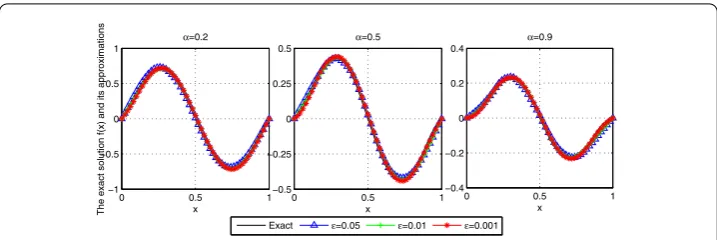
Figure shows the comparisons between the exact solution and its regularized so-lution for various noise levels ε= ., ., . in the case of α = ., ., .. The iterative step m = ,, ,, ,, for α = ., in the case of α = ., m= ,, ,, , andm= ,, ,, ,, forα= ..
Example Consider the following discontinuous function:
f(x) = ⎧ ⎪ ⎪ ⎪ ⎪ ⎪ ⎪ ⎪ ⎪ ⎨ ⎪ ⎪ ⎪ ⎪ ⎪ ⎪ ⎪ ⎪ ⎩
, ≤x≤., , . <x≤., , . <x≤., –, . <x≤., , . <x≤.
(.)
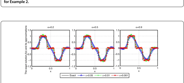
Figure shows the comparison between the exact solution and its regularized so-lution for various noise levels ε= ., ., . in the case of α = ., ., .. The iterative step m= ,, ,, , for α = ., in the case of α = ., m= ,, ,, ,, andm= ,, ,, ,, forα= ..
it-Figure 2 The comparison of numerical effects between the exact solution and its regularized solution for Example 2.
Figure 3 The comparison of numerical effects between the exact solution and its regularized solution for Example 3.
erative step m= ,, ,,, ,, forα = ., in the case ofα= ., m= ,, ,,, ,, andm= ,, ,,, ,, forα= ..
In Figures -, we see that the smallerεandα, the better the regularized solution is. Moreover, we see that thea posterioriparameter choice also works well.
Example Take source functionf(x,y) =xy.
In Example , we takeT = .,M=M= ,N= andl=l= . Figure shows the comparison between the exact solution and its regularized solution for various noise levelsε= ., . in the case ofα= .. The iterative stepm= , forε= ., m= ,, when the error levelε= ..
Example Take source functionf(x,y) =sin(x)sin(y) +sin(x)sin(y).
In Example , we takeT= ,M=M= ,N= andl=l=π. Figure shows the comparison between the exact solution and its regularized solution for various noise levels
ε= ., . in the case ofα= .. The iterative stepm= forε= .,m= when
error levelε= ..
Figure 4 The comparison of numerical effects between the exact solution and its regularized solution for Example 4.
Figure 5 The comparison of numerical effects between the exact solution and its regularized solution for Example 5.
6 Conclusion
two regularization methods to identify the spatial variable source for the time-fraction diffusion equation. In [], the authors used quasi-reversibility regularization methods to identify the spatial variable source for the time-fraction diffusion equation. From [], under thea prioriregularization parameter choice rule, the authors found the orders of error estimate convergence areO(δ
p
p+) ( <p≤) andO(δ) (p> ) and under thea posterioriregularization parameter choice rule, the authors found the orders of error es-timate convergence areO(δ
p
p+) ( <p≤) andO(δ) (p> ). In [], under thea priori anda posterioriregularization parameter choice rules, the authors found the orders of error estimate convergence areO(δ
p
p+) ( <p≤) andO(δ) (p> ), but in our paper, under thea priorianda posterioriregularization parameter choice rules, we found the order of error estimate convergence isO(δp+p ). Comparing references [, ], under the a posterioriregularization parameter choice, asp> , the authors found the error esti-mate convergence isO(δ) (p> ), which is a saturating phenomenon,i.e., if we add the smoothness of the solution, the error estimate order does not improve. In our method, the error estimate convergence isO(δ
p
p+), which does not appear to be a saturating
phe-nomenon. Finally, three numerical results show that the Landweber iterative method is very effective for this kind of ill-posed problems.
Acknowledgements
The authors would like to thanks the editor and the referees for their valuable comments and suggestions, that improved the quality of our paper.
Funding
The work is supported by the National Natural Science Foundation of China (11561045, 11501272) and the Doctor Fund of Lan Zhou University of Technology.
Abbreviations Not applicable.
Availability of data and materials Not applicable.
Competing interests
The authors declare that they have no competing interests.
Authors’ contributions
The main idea of this paper was proposed by FY. Y-PR prepared the manuscript initially and performed all the steps of the proofs in this research. All authors read and approved the final manuscript.
Publisher’s Note
Springer Nature remains neutral with regard to jurisdictional claims in published maps and institutional affiliations.
Received: 21 June 2017 Accepted: 1 November 2017
References
1. Chen, W, Ye, LJ, Sun, HG: Fractional diffusion equations by the Kansa method. Comput. Math. Appl.59, 1614-1620 (2010)
2. Agarwal, RP, Asma, Lupulescu, V, O’Regan, D: Fractional semilinear equations with causal operators. Rev. R. Acad. Cienc. Exactas Fís. Nat., Ser. A Mat.111, 257-269 (2017)
3. Yu, Z, Lin, J: Numerical research on the coherent structure in the viscoelastic second-order mixing layers. Appl. Math. Mech.19, 671-677 (1998)
4. Laskin, N, Lambadaris, I, Harmantzis, FC, Devetsikiotis, M: Fractional Lévy motion and its application to network traffic modeling. Comput. Netw.40(3), 363-375 (2002)
5. Scher, H, Montroll, EW: Anomalous transit-time dispersion in amorphous. Phys. Rev. B12(6), 2455-2477 (1975) 6. Szabo, TL, Wu, J: A model for longitudinal and shear wave propagation in viscoelastic media. J. Acoust. Soc. Am.
107(5), 2437-2446 (2000)
7. Gorenflo, R, Mainardi, F, Moretti, D, Pagnini, G, Paradisi, P: Discrete random walk models for space-time fractional diffusion. Chem. Phys.284, 521-541 (2002)
9. Sokolov, IM, Klafter, J, Blumen, A: Fractional kinetics. Phys. Today55, 48-54 (2002)
10. Lopushanska, H, Lopushansky, A, Myaus, O: Inverse problems of periodic spatial distributions for a time fractional diffusion equation. Electron. J. Differ. Equ.2016, 14 (2016)
11. Nemat, D: Numerical study of entropy generation for forced convection flow and heat transfer of a Jeffrey fluid over a stretching sheet. Alex. Eng. J.53, 769-778 (2014)
12. Mendes, RV: A fractional calculus interpretation of the fractional volatility model. Nonlinear Dyn.55, 395-399 (2009) 13. Muhammad, MB, Tehseen, A, Mohammad, MR: Entropy generation as a practical tool of optimisation for
non-Newtonian nanofluid flow through a permeable stretching surface using SLM. J. Comput. Des. Eng.4, 21-28 (2017)
14. Wyss, W: The fractional diffusion equation. J. Math. Phys.27(11), 2782-2785 (1986)
15. Schneider, WR, Wyss, W: Fractional diffusion and wave equations. J. Math. Phys.30(1), 134-144 (1989)
16. Agrawal, OP: Solution for a fractional diffusion-wave equation defined in a bounded domain. Nonlinear Dyn.29(1), 145-155 (2002)
17. Murio, DA: Time fractional IHCP with Caputo fractional derivatives. Comput. Math. Appl.56(9), 2371-2381 (2008) 18. Murio, DA: Implicit finite difference approximation for time-fractional diffusion equations. Comput. Math. Appl.56(4),
1138-1145 (2008)
19. Zhuang, P, Liu, F: Implicit difference approximation for the time fractional diffusion equation. J. Appl. Math. Comput.
22(3), 87-99 (2006)
20. Zhang, H, Liu, FW, Anh, V: Galerkin finite element approximation of symmetric space-fractional partial differential equations. Appl. Math. Comput.217(6), 2534-2545 (2010)
21. Li, XJ, Xu, CJ: Existence and uniqueness of the weak solution of the space-time fractional diffusion equation and spectral method approximation. Commun. Comput. Phys.8(5), 1016-1051 (2010)
22. Fulger, D, Scalas, E, Germano, G: Monte Carlo simulation of uncoupled continuous-time random walks yielding a stochastic solution of the space-time fractional diffusion equation. Phys. Rev. E77(2), 021122 (2008)
23. Tatar, S, Ulusoy, S: An inverse coefficient problem for a nonlinear reaction diffusion equation with a nonlinear source. Electron. J. Differ. Equ.2015, 245 (2015)
24. Tuan, NH, Kirane, M, Luu, VCH, Bin-Mohsin, B: A regularization method for time-fractional linear inverse diffusion problems. Electron. J. Differ. Equ.2016, 290 (2016)
25. Liu, JJ, Yamamoto, M: A backward problem for the time-fractional diffusion equation. Appl. Anal.89(11), 1769-1788 (2010)
26. Murio, DA, Mejía, CE: Source terms identification for time fractional diffusion equation. Rev. Colomb. Mat.42(1), 25-46 (2008)
27. Wang, JG, Wei, T, Zhou, YB: Tikhonov regularization method for a backward problem for the time-fractional diffusion equation. Appl. Math. Model.37(18), 8518-8532 (2013)
28. Zhang, Y, Xu, X: Inverse source problem for a fractional diffusion equation. Inverse Probl.27(3), 035010 (2011) 29. Sakamoto, K, Yamamoto, M: Initial value/boundary value problems for fractional diffusion-wave equations and
applications to some inverse problems. J. Math. Anal. Appl.382(1), 426-447 (2011)
30. Yang, F, Fu, CL: A simplified Tikhonov regularization method for determining the heat source. Appl. Math. Model.
34(11), 3286-3299 (2010)
31. Dou, FF, Fu, CL: Determining an unknown source in the heat equation by a wavelet dual least squares method. Appl. Math. Lett.22, 661-667 (2009)
32. Farcas, A, Lesnic, D: The boundary-element method for the determination of a heat source dependent on one variable. J. Eng. Math.54, 375-388 (2006)
33. Johansson, T, Lesnic, D: Determination of a spacewise dependent heat source. J. Comput. Appl. Math.20, 966-980 (2007)
34. Liu, CH: A two-stage LGSM to identify time-dependent heat source through an internal measurement of temperature. Int. J. Heat Mass Transf.52, 1635-1642 (2009)
35. Dou, FF, Fu, CL, Yang, FL: Optimal error bound and Fourier regularization for identifying an unknown source in the hear equation. J. Comput. Appl. Math.230, 728-737 (2009)
36. Zhang, ZQ, Wei, T: Identifying an unknown source in time-fractional diffusion equation by a truncation method. Appl. Math. Comput.219(11), 5972-5983 (2013)
37. Wang, JG, Zhou, YB, Wei, T: Two regularization methods to identify a space-dependent source for the time-fractional diffusion equation. Appl. Numer. Math.68, 39-57 (2013)
38. Wang, JG, Wei, T: Quasi-reversibility method to identify a space-dependent source for the time-fractional diffusion equation. Appl. Math. Model.39, 6139-6149 (2015)
39. Landweber, L: An iteration formula for Fredholm integral equations of the first kind. Am. J. Math.73(3), 615-624 (1951) 40. Podlubny, I: Fractional Differential Equations. Academic Press, San Diego (1999)
41. Haubold, HJ, Mathai, AM, Saxena, RK: Mittag-Leffler functions and their applications. J. Appl. Math.2011, Article ID 298628 (2011)
42. Pollard, H: The completely monotonic character of the Mittag-Leffler functionEα(–x). Bull. Am. Math. Soc.54,
1115-1116 (1948)
43. Wei, T, Wang, JG: A modified quasi-boundary value method for the backward time-fractional diffusion problem. ESAIM: Math. Model. Numer. Anal.48(2), 603-621 (2014)