Doctoral School in Environmental Engineering
High Order Direct Arbitrary-Lagrangian-Eulerian (ALE)
Finite Volume Schemes for Hyperbolic Systems
on Unstructured Meshes
Walter Boscheri
UNIVERSIT ´
A DEGLI STUDI DI TRENTO
Dipartimento di Ingegneria Civile, Ambientale e Meccanica
Department of Civil, Environmental and Mechanical Engineering,
University of Trento.
Academic year
2014/2015
.
Internal supervisor
:
Prof. Dr.-Ing. Michael Dumbser
External supervisors
:
Prof. Dr. Claus-Dieter Munz
IAG-Stuttgart (Germany)
:
Prof. Dr. Bruno Despr´
es
University of Paris (France)
Ai miei genitori Anna Maria e Roberto
“
dos est magna parentium virtus
”
This thesis has been developed during the three-year Doctoral program of the
Doctoral School in Environmental Engineering at the Department of Civil,
En-vironmental and Mechanical (DICAM) Engineering of the University of Trento.
The presented research has been financed by the European Research Council
(ERC) under the European Union’s Seventh Framework Programme
(FP7/2007-2013) with the research project
STiMulUs
, ERC Grant agreement no. 278267.
Most of the work has been carried out at DICAM (Trento) under the
super-vision of Prof. Dr.-Ing. Michael Dumbser. Furthermore I spent two months
(August 2013 - September 2013) at the Department of Physics of the Notre
Dame University (South Bend, IN - USA) for a collaboration with Prof.
Din-shaw Balsara, while for three months (September 2014 - November 2014) my
work took place at the Institute de Math´
ematiques de Toulouse (Toulouse,
France) with Dr. Rapha¨
el Loub`
ere in order to be assigned with the
Doctor
Europaeus
label.
Some of the two-dimensional simulations shown in this thesis have been run on
the AMD Opteron cluster of the
STiMulUs
project located in Povo (Trento,
Italy), while the rest of the numerical results have been collected using the
Su-perMUC supercomputer of the Leibniz Rechenzentrum (LRZ) in Munich
(Ger-many), for which we gained access under the project “STiMulUs - Lagrangian
Space-Time Methods for Multi-Fluid Problems on Unstructured Meshes”,
pro-posals no. 2012071312, 2013091889 and 2014112638.
Trento, January 2015
Acknowledgments
I would like to thank Prof. Dumbser for his outstanding supervision as well as
for his friendship, that allowed my research to be carried out within excellent
working conditions.
Many thanks also to Prof. Balsara and Dr. Loub`
ere for the collaborations done
together and to the external supervisors Prof. Munz and Prof. Despr´
es, who
spent part of their time to read and review this thesis.
Contents
Symbols
xi
Abbreviations
xiii
Abstract
xiv
1
Introduction
1
1.1
High order finite volume methods on fixed grids . . . .
2
1.2
Lagrangian methods on moving meshes
. . . .
4
1.3
Towards high order ALE ADER-WENO schemes . . . .
7
2
High Order ALE One-Step ADER-WENO Finite Volume Schemes
11
2.1
Finite volume framework on moving unstructured meshes . . .
11
2.2
Polynomial WENO reconstruction . . . .
13
2.3
Local space-time Galerkin predictor on moving curved meshes .
19
2.3.1
Local Continuous Galerkin (CG) predictor . . . .
24
2.3.2
Local Discontinuous Galerkin (DG) predictor . . . .
26
2.4
Mesh motion . . . .
28
2.5
High order ALE finite volume schemes . . . .
30
2.5.1
Formulation for non-conservative systems . . . .
35
2.5.2
Formulation for conservative systems . . . .
37
3
Mesh Motion
39
3.1
The Lagrangian step: node solvers . . . .
40
3.1.1
The node solver of Cheng and Shu
N S
cs
. . . .
41
3.1.2
The node solver of Maire
N S
m
. . . .
42
3.1.3
The node solver of Balsara et al.
N S
b
. . . .
44
3.2
The rezoning step . . . .
46
4
Algorithm Efficiency Improvements
51
4.1
Time-accurate local time stepping on moving meshes . . . .
54
4.1.1
High order WENO reconstruction for local time stepping
55
4.1.2
Mesh motion with local time stepping . . . .
58
4.1.3
Finite volume scheme with local time stepping . . . . .
59
4.1.4
Description of the high order Lagrangian LTS algorithm
in multiple space dimensions
. . . .
64
4.2
Genuinely multidimensional HLL Riemann solvers for ALE
meth-ods . . . .
67
4.3
Quadrature-free ALE ADER schemes
. . . .
70
4.4
Direct ALE ADER-MOOD finite volume schemes . . . .
76
4.4.1
MOOD paradigm as stabilization technique . . . .
78
4.4.2
The MOOD loop . . . .
81
5
Applications to Hyperbolic Systems
83
5.1
The Euler equations of compressible gas dynamics
. . . .
83
5.1.1
Numerical convergence studies
. . . .
84
5.1.2
The Sod shock tube problem . . . .
87
5.1.3
Multidimensional explosion problem . . . .
88
5.1.4
The Kidder problem . . . .
89
5.1.5
The Saltzman problem . . . .
90
5.1.6
The Sedov problem . . . .
93
5.1.7
The Noh problem . . . .
94
5.1.8
The Gresho vortex problem . . . .
95
5.1.9
The Taylor-Green vortex problem
. . . .
96
5.1.10 The two-dimensional double Mach reflection problem . .
96
5.1.11 Mono-material triple point problem
. . . .
97
5.1.12 Multi-material flow . . . .
97
5.2
The ideal magnetohydrodynamics (MHD) equations
. . . .
101
5.2.1
Numerical convergence studies
. . . .
102
5.2.2
The MHD rotor problem . . . .
103
5.2.3
The MHD blast wave problem
. . . .
105
5.3
The relativistic MHD equations (RMHD) . . . .
105
5.3.1
Large Amplitude Alfv´
en wave . . . .
106
5.3.2
The RMHD rotor problem . . . .
107
5.3.3
The RMHD blast wave problem
. . . .
108
5.4
The Baer-Nunziato model of compressible two-phase flows . . .
108
5.4.1
Numerical convergence studies
. . . .
110
Contents
5.4.3
Explosion problems . . . .
114
5.4.4
Two-Dimensional Riemann Problems . . . .
115
6
Numerical Results
117
6.1
The Euler equations of compressible gas dynamics
. . . .
119
6.1.1
Numerical convergence studies
. . . .
119
6.1.2
The Sod shock tube problem . . . .
126
6.1.3
Multidimensional explosion problem . . . .
133
6.1.4
The Kidder problem . . . .
138
6.1.5
The Saltzman problem . . . .
144
6.1.6
The Sedov problem . . . .
146
6.1.7
The Noh problem . . . .
150
6.1.8
The Gresho vortex problem . . . .
157
6.1.9
The Taylor-Green vortex problem
. . . .
159
6.1.10 Mono-material triple point problem
. . . .
160
6.1.11 Multi-material flow . . . .
164
6.1.12 The two-dimensional double Mach reflection problem . .
167
6.1.13 Efficiency comparison
. . . .
169
6.2
The ideal magnetohydrodynamics (MHD) equations
. . . .
173
6.2.1
Numerical convergence studies
. . . .
173
6.2.2
The MHD rotor problem . . . .
173
6.2.3
The MHD blast wave problem
. . . .
176
6.3
The relativistic MHD equations (RMHD) . . . .
180
6.3.1
Large Amplitude Alfv´
en wave . . . .
181
6.3.2
The RMHD rotor problem . . . .
182
6.3.3
The RMHD blast wave problem
. . . .
183
6.4
The Baer-Nunziato model of compressible two-phase flows . . .
183
6.4.1
Numerical convergence studies
. . . .
187
6.4.2
Riemann problems . . . .
187
6.4.3
Explosion problems . . . .
190
6.4.4
Two-Dimensional Riemann Problems . . . .
191
6.4.5
Computational efficiency comparison of Eulerian and ALE
schemes . . . .
197
7
Conclusions and Outlook
203
A Basis Functions
207
A.1 Space basis functions . . . .
207
B Positivity preserving technique
213
C Geometric Conservation Law (GCL)
217
D Boundary conditions
221
Bibliography
225
List of Tables
250
Symbols
Symbols
c
Speed of sound
d
Number of space dimensions
i
Element index
j
Neighbor element index
k
Node index
M
Maximum degree of the reconstruction
n
Current time level
n
+ 1
Future time level
p
Pressure
t
Time
T
Control volume
u
Velocity component in
x
-direction
v
Velocity component in
y
-direction
w
Velocity component in
z
-direction
x
Horizontal direction in the physical system
y
Lateral direction in the physical system
z
Vertical direction in the physical system
β
Linear basis function
γ
Ratio of specific heats
δij
Kronecker symbol
∆
t
Timestep
ρ
Density
ρE
Total energy per mass unit
ε
∗
Internal energy per mass unit
θ
Space-time basis function and test function
ψ
Space basis function
Ψ
Integration path
ξ
Horizontal direction in the reference system
η
Lateral direction in the reference system
ζ
Vertical direction in the reference system
χ1, χ2
Face parameters on the element boundary
Ω
Computational domain
B
Non-conservative nonlinear flux tensor
F
Conservative nonlinear flux tensor
I
Identity matrix
n
Element boundary normal vector in space
˜
n
Element boundary normal vector in space and time
A
Algorithm efficiency
N S
cs
Node solver of Cheng and Shu
N S
m
Node solver of Maire
N S
b
Node solver of Balsara
N
i
Neumann neighborhood of element
i
O
Order of the scheme
V
k
Voronoi neighborhood of node
k
V
i
Voronoi neighborhood of element
i
Q
Vector of conserved variables
U
Vector of primitive variables
S
Algebraic source term
v
Vector of the local fluid velocity
V
Vector of the local mesh velocity
X
k
Vertex physical coordinates in space
x
Physical spatial coordinate vector
˜
x
Physical space-time coordinate vector
ξ
Reference spatial coordinate vector
˜
ξ
Reference space-time coordinate vector
q
h
High order space-time predictor solution
Abbreviations
Abbreviations
ADER
Arbitrary high order scheme using derivatives
ALE
Arbitrary-Lagrangian-Eulerian scheme
CG
Continuous Galerkin method
CFL
Courant-Friedrichs-Levy number
CPU
Central processing unit
DG
Discontinuous Galerkin method
ENO
Essentially non-oscillatory
FV
Finite Volume
GRP
Generalized Riemann problem
HD
Hydrodynamics
IC
Initial condition
LTS
Local time stepping
MHD
Magneto-Hydrodynamics
MOOD
Multi-dimensional optimal order detection
ODE
Ordinary differential equation
PDE
Partial differential equation
TVD
Total variation diminishing
Abstract
In this work we develop a new class of high order accurate
Arbitrary-Lagrangian-Eulerian (ALE) one-step finite volume schemes for the solution
of nonlinear systems of conservative and non-conservative hyperbolic partial
differential equations. The numerical algorithm is designed for two and three
space dimensions, considering
moving
unstructured triangular and tetrahedral
meshes, respectively.
As usual for finite volume schemes, data are represented within each control
volume by piecewise constant values that evolve in time, hence implying the
use of some strategies to improve the order of accuracy of the algorithm. In our
approach high order of accuracy in space is obtained by adopting a
WENO
re-construction
technique, which produces piecewise polynomials of higher degree
starting from the known cell averages. Such spatial high order accurate
recon-struction is then employed to achieve high order of accuracy also in time using
an element-local space-time
finite element predictor
, which performs a
one-step time discretization. Specifically, we adopt either the continuous Galerkin
(CG) predictor, which does not allow discontinuities in time and is suitable for
smooth time evolutions, or the discontinuous Galerkin (DG) predictor which
can handle stiff source terms that might produce jumps in the local space-time
solution. Since we are dealing with moving meshes the elements deform while
the solution is evolving in time, hence making the use of a reference system very
convenient. Therefore, within the space-time predictor, the physical element is
mapped onto a reference element using a high order isoparametric approach,
where the space-time basis and test functions are given by the Lagrange
inter-polation polynomials passing through a predefined set of space-time nodes.
The computational mesh continuously changes its configuration in time,
follow-ing as closely as possible the flow motion. The entire mesh motion procedure
is composed by three main steps, namely the Lagrangian step, the rezoning
step and the relaxation step. In order to obtain a continuous mesh
configura-tion at any time level, the mesh moconfigura-tion is evaluated by assigning each node of
the computational mesh with a unique velocity vector at each timestep. The
node solver
algorithm preforms the Lagrangian stage, while we rely on a
re-zoning algorithm
to improve the mesh quality when the flow motion becomes
very complex, hence producing highly deformed computational elements. A
so-called
relaxation algorithm
is finally employed to partially recover the
Abstract
velocity. Once the vertex velocity and thus the new node location has been
determined, the old element configuration at time
t
n
is connected with the new
one at time
t
n+1
with
straight edges
to represent the local mesh motion, in
order to maintain algorithmic simplicity.
The final
ALE finite volume scheme
is based directly on a space-time
con-servation formulation of the governing system of hyperbolic balance laws. The
nonlinear system is reformulated more compactly using a space-time divergence
operator and is then integrated on a moving space-time control volume. We
adopt a linear parametrization of the space-time element boundaries and
Gaus-sian quadrature rules of suitable order of accuracy to compute the integrals.
In our algorithm either a simple and robust Rusanov-type numerical flux or a
more sophisticated and less dissipative Osher-type numerical flux is employed.
We apply the new high order direct ALE finite volume schemes to several
hyper-bolic systems, namely the multidimensional Euler equations of compressible gas
dynamics, the ideal classical and relativistic magneto-hydrodynamics (MHD)
equations and the non-conservative seven-equation Baer-Nunziato model of
compressible multi-phase flows with stiff relaxation source terms. Numerical
convergence studies as well as several classical test problems will be shown to
assess the accuracy and the robustness of our schemes.
Furthermore we focus on the following issues to improve the algorithm
ef-ficiency: the time evolution, the numerical flux computation across element
boundaries and the high order WENO reconstruction procedure.
First, a
time-accurate local time stepping
(LTS) algorithm for unstructured
triangu-lar meshes is derived and presented, where each element can run at its own
optimal time step, given by a local CFL stability condition. Then, we propose
a new and efficient
quadrature-free
formulation for the flux computation, in
which the space-time boundaries of each element are split into simplex
sub-elements. This leads to space-time normal vectors as well as Jacobian matrices
that are constant within each sub-element, hence allowing the flux integrals
to be evaluated on the space-time reference control volume once and for all
analytically during a preprocessing step. Finally, we consider the very new
a posteriori MOOD paradigm
, recently proposed for the Eulerian framework,
to overcome the expensive WENO approach on moving meshes. The MOOD
technique requires the use of only one central reconstruction stencil because
the limiting procedure is carried out
a posteriori
instead of
a priori
, as done in
1 Introduction
Many real world processes are modeled using time-dependent partial
differen-tial equations (PDE), which are based on the conservation of some physical
quantities. Therefore these mathematical and physical models are typically
addressed as
conservation laws
and they cover a wide range of phenomena,
such as environmental and meteorological flows, hydrodynamic and
thermody-namic problems, plasma flows as well as the dythermody-namics of many industrial and
mechanical processes. In any case the governing equations can generally be
solved using either an
Eulerian
or a
Lagrangian
approach. In the first case the
fluid flow is observed and computed in a fixed reference system, while in the
latter case the reference system is moving
together
with the local fluid velocity.
In general any conservation law assumes that the modeled medium is a
contin-uum and describes the evolution of the
conserved quantity
u
(
x
, t
) in the control
volume
ω
, which can be chosen arbitrarily. The conserved quantity depends
both on space (
x
) and time (
t
) and any change of
u
, i.e. the time evolution
of
u
, is assumed to be due to some
fluxes
F
(
u
) across the boundary
∂ω
of the
control volume and, in some cases, also to a so-called
source term
S
(
u
) that
may affect the evolution of
u
by either increasing or decreasing the conserved
quantity. A very general formulation for a conservation law reads
∂
∂t
Z
ω
u dV
+
Z
∂ω
F
(
u
)
n dS
=
Z
ω
S
(
u
)
,
(1.1)
where
n
represents the outward pointing unit normal vector on the boundary
∂ω
. The above expression must be valid for any control volume, hence leading
to the following partial differential equation:
∂u
∂t
+
∇ ·
F
(
u
) =
S
(
u
)
,
(1.2)
where Gauss’ theorem has been used to rewrite the boundary integral as the
volume integral of the divergence of the fluxes
∇ ·
F
(
u
).
The quantity
u
might also be a vector, hence involving more conserved
and total energy. As a consequence we obtain a
system of conservation laws
,
whenever the quantity
u
is given by a vector. In this case a system matrix
A
can be defined as
A
=
∂F
∂u
n
(1.3)
and the system is considered
hyperbolic
if for all
n
all eigenvalues of matrix
A
are real and if a complete set of eigenvectors exists.
This work focuses on the solution of hyperbolic systems of conservation laws of
the form (1.2), considering a Lagrangian-like approach, where the control
vol-ume
ω
(
t
) is moving and therefore is time-dependent. Specifically, our task is
to design high order accurate finite volume schemes for the solution of
hyper-bolic systems adopting an
Arbitrary-Lagrangian-Eulerian
approach. Section
1.1 provides a general overview of high order numerical methods for the
solu-tion of hyperbolic PDEs in the Eulerian framework, while Secsolu-tion 1.2 presents
a literature review of the state-of-the-art in the field of Lagrangian numerical
schemes. Finally, Section 1.3 provides the introduction to this work.
1.1 High order finite volume methods on fixed grids
The Eulerian approach implies the introduction of nonlinear convective terms
in the governing equations because the flow is observed in a fixed reference
system, which does not neither change nor move in time. These terms are
considered within the flux term
F
(
u
) of the conservation law (1.2). A lot of
research has been carried out in the past decades in order to solve conservation
laws of the form (1.2) numerically, starting from the one-dimensional case. A
very famous and widespread approach is given by
Godunov
-type finite volume
methods [133,240], where the discrete solution is stored as constant data within
each control volume of the computational mesh and is evolved in time by using
the integral form of the conservation law (1.1). Since the discrete solution in
general exhibits jumps at the element interfaces, the introduction of numerical
fluxes across the discontinuities of each cell is necessary. Godunov suggested to
obtain these numerical fluxes by solving
Riemann problems
at each interface.
1.1 High order finite volume methods on fixed grids
Munz in [113] with the introduction of the HLLEM Riemann solver, where the
intermediate state was assumed piecewise linear instead of piecewise constant.
Another well-known improvement of the original HLL scheme is due to Toro et
al. in [231] with the design of the HLLC Riemann solvers that use an enhanced
wave model that is able to capture also the intermediate contact wave. In [190]
Osher et al. introduced a class of approximate Riemann solvers based on path
integrals, where the paths were obtained by an approximation of the solution
of the Riemann problem by rarefaction fans.
A simpler and more general
version of the Osher flux has recently been forwarded by Dumbser and Toro
in [106, 107]. All those one-dimensional Riemann solvers can be used even in
two- and three-dimensional problems, where the discontinuities are resolved at
each boundary of the control volume along the normal direction.
In order to design
high order accurate
finite volume numerical schemes, a high
order reconstruction operator in space is needed as well as a time evolution
of the conserved quantities that allows the method to achieve high order of
accuracy even in time. Since linear monotone schemes are at most of order
one, as stated by the Godunov theorem [134], a first contribution for the
im-provement of the order of accuracy has been provided by the class of second
order accurate TVD schemes, which adopts a linear reconstruction in space and
time, like the MUSCL scheme of van Leer [241] and the second order method
of Barth and Jespersen on unstructured meshes [30]. Later on nonlinear ENO
reconstructions on unstructured grids have been introduced [4, 217] as well as
WENO reconstructions [126, 144, 215]. Once the high order spatial
reconstruc-tion is available, a suitable time stepping technique has to be used to guarantee
the final order of accuracy. Runge-Kutta (RK) methods perform a multi-stage
time-integration to evolve the numerical solution from the current time level
t
n
to the next time level
t
n+1
. The higher is the order of accuracy, the higher
piecewise constants as in the original formulation of Godunov [134]. The first
ADER algorithms [151, 178, 210, 211, 222, 223, 233, 234] follow the concept of
Ben-Artzi and Falcovitz [31] based on the solution of the generalized Riemann
problem (GRP) at zone boundaries. The time evolution is carried out by using
repeatedly the governing conservation law in differential form to replace time
derivatives by space derivatives, which is the so-called Cauchy-Kovalewski or
Lax-Wendroff procedure.
The idea behind the GRP approach is a
tempo-ral Taylor series expansion of the state at the interface. However, problems
arise when the solution is discontinuous. Since in general jumps are admitted
at element boundaries, conventional homogeneous Riemann problems for the
state and all space derivatives have first to be solved at the interface, then the
obtained results are plugged into the Cauchy-Kovalewski procedure to obtain
high order accurate time derivatives. The resulting ADER schemes are
one-step fully discrete and of arbitrary order of accuracy in space and time, and
have been successfully used in the framework of both finite volume (FV) and
Discontinuous Galerkin (DG) methods, see [102, 103, 105, 210, 211]. An efficient
quadrature-free approach for the numerical flux integration has been proposed
in [103].
The most recent ADER methods [27, 28, 94, 98] evolve the spatially high
or-der accurate reconstruction polynomial locally in time using a weak integral
formulation of the conservation law in space-time, hence obtaining space-time
accurate representation of the solution within a cell. This most recent version
of the ADER schemes is more similar to the original ENO scheme proposed by
Harten et al. [138], since it first evolves the data in each element by solving a
lo-cal Cauchy problem in the small, i.e. without accounting for the neighbor cells,
and then solves the interactions at the zone boundaries. The main advantages
of this time evolution are: (i) the cumbersome Cauchy-Kovalewski procedure
is no more needed, and (ii) the resulting technique can handle very general and
different hyperbolic systems of conservation laws. Furthermore stiff sources are
also treated properly, as highlighted in [99, 141].
1.2 Lagrangian methods on moving meshes
1.2 Lagrangian methods on moving meshes
discontinuities to be precisely located and tracked during the computation,
achieving a much more accurate resolution of these waves compared to
classi-cal Eulerian methods on fixed grids. For this reason a lot of efforts has been
made in the last decades in order to develop Lagrangian methods. Already
John von Neumann and Richtmyer were working on Lagrangian schemes in
the 1950ies [242], using a formulation of the governing equations in primitive
variables, which was also used later in [32, 51]. However, most of the modern
Lagrangian finite volume schemes use the conservation form of the equations
based on the physically conserved quantities like mass, momentum and total
energy in order to compute shock waves properly, see e.g. [53,172,182,216].
La-grangian schemes can be also classified according to the location of the physical
variables on the mesh: when all variables are defined on a collocated grid the
so-called
cell-centered
approach is adopted [71, 171–173, 202], while in the
stag-gered mesh
approach [167, 168] the velocity is defined at the cell interfaces and
the other variables at the cell center.
Cell-centered Lagrangian Godunov-type schemes of the Roe-type and of the
HLL-type for the Euler equations of compressible gas dynamics have first been
considered by Munz in [182]. A cell-centered Godunov-type scheme has also
been introduced by Carr´
e et al. in [53], who developed a Lagrangian finite
volume algorithm on general multidimensional unstructured meshes. The
re-sulting finite volume scheme is node based and compatible with the mesh
dis-placement. In the work of Despr´
es et al. [77,78] the physical part of the system
of equations is coupled and evolved together with the geometrical part, hence
obtaining a weakly hyperbolic system of conservation laws that is solved using a
node-based finite volume scheme. Furthermore they presented a cell-centered
Lagrangian method [71] that is translation invariant and suitable for curved
meshes.
In [169–171] Maire proposed first and second order accurate
[48, 125, 203, 244] purely Lagrangian and Arbitrary-Lagrangian-Eulerian (ALE)
numerical schemes with remapping for multi-phase and multi-material flows are
discussed. All the Lagrangian schemes listed so far are at most second order
accurate in space and time.
Higher order of accuracy in space was first achieved in [65–67,163] by Cheng and
Shu, who introduced a third order accurate essentially non-oscillatory (ENO)
reconstruction operator into Godunov-type Lagrangian finite volume schemes.
High order of accuracy in time was guaranteed either by the use of a
Runge-Kutta or by a Lax-Wendroff-type time stepping. The mesh velocity is simply
computed as the arithmetic average of the corner-extrapolated values in the
cells adjacent to a mesh vertex. Such a node solver algorithm is very simple and
general and can be easily applied to different complicated nonlinear systems
of hyperbolic PDE in multiple space dimensions. Cheng and Toro [68] also
investigated Lagrangian ADER-WENO schemes in one space dimension. In the
finite element framework high order Lagrangian schemes have been developed
for example by Scovazzi et al. [187, 213] and also by Dobrev et al. [82–84], who
solved the equations for Lagrangian hydrodynamics using high order curvilinear
finite element methods.
1.3 Towards high order ALE ADER-WENO schemes
1.3 Towards high order ALE ADER-WENO schemes
The aim of this work is to design a new family of high order accurate
Arbitrary-Lagrangian-Eulerian (ALE) one-step ADER-WENO finite volume schemes for
the solution of nonlinear systems of conservative and non-conservative
hyper-bolic partial differential equations.
The work is based on the already existing high order ADER finite volume
solver [94,98] mentioned in Section 1.1, which is used here as a starting point for
the development of the new Lagrangian algorithms. From Section 1.2 we know
that no better than third order accurate non-oscillatory Lagrangian schemes
have ever been proposed on unstructured meshes in two and three space
dimen-sions, hence leading to a challenging task that matches the research frontier of
numerical methods on moving mesh. Furthermore, the new algorithm emerging
from this work will be so
general
that it will be applicable to a wide range of
scientific fields, since it is based on a very general formulation of the governing
PDE, which many hyperbolic systems can be cast into.
The first contribution to this new class of numerical methods, which will be
ad-dressed as
direct ALE ADER-WENO schemes
, has been presented by Dumbser
et al. in [108], where the authors proposed the first one-dimensional high order
ALE ADER-WENO finite volume schemes for hyperbolic balance laws with
stiff source terms. In this case high order of accuracy in time was achieved by
using the local space-time Galerkin predictor method introduced in [98, 141]
for the Eulerian case, whereas a high order WENO reconstruction algorithm
was used to obtain high order of accuracy in space.
schemes have been applied to conservative and non-conservative hyperbolic
systems on unstructured tetrahedral moving meshes, while in [44] Boscheri
and Dumbser introduce a quadrature-free formulation for the numerical flux
computation in the ALE context. In order to reduce the computational efforts,
which is typically higher for Lagrangian schemes than for Eulerian methods,
in [43, 93] the first high order time-accurate local time stepping ALE
ADER-WENO schemes have been presented in one and two space dimensions, while
in [45] the expensive WENO reconstruction procedure has been replaced with
the very recently developed MOOD paradigm [69,79,81,165], which requires the
use of only one central reconstruction stencil because the limiting procedure is
carried out
a posteriori
instead of
a priori
, as done in the WENO formulation.
The rest of the work is structured as follows. In Chapter 2 we describe in
detail the new high order ALE ADER-WENO finite volume schemes,
consid-ering what has been done in [39, 40, 96]. The algorithm will be presented in a
very general way, treating both conservative and non-conservative hyperbolic
systems as well as the presence of algebraic source terms which are allowed
to be stiff. Next, Chapter 3 focuses on the techniques used to carry out the
mesh motion, i.e. the numerical strategies adopted to evaluate the mesh
veloc-ity and consequently to compute the new node location. Three different node
solvers will be considered, according to [41], and a rezoning technique with a
relaxation algorithm will also be detailed. Chapter 4 aims at introducing some
modifications of the direct ALE WENO algorithm, presented in Chapter 2,
in order to improve the overall algorithm efficiency. Specifically, we present
(i) a local time stepping (LTS) algorithm for moving unstructured triangular
meshes [43], (ii) the genuinely multidimensional HLL Riemann solvers for the
flux computation in the ALE ADER-WENO framework according to [38], (iii)
an efficient quadrature-free approach for the numerical flux integration [44] and
finally (iv) the MOOD version [45] of our original ALE ADER scheme, which
adopts an efficient
a posteriori
limiting technique. In Chapter 5 several
hyper-bolic systems of conservation laws will be described as well as the associated
test cases used to validate our new finite volume schemes. The corresponding
numerical results are given in Chapter 6, where we present some of the
numer-ical simulations that have been run during the last three years of our research
activity.
For a more detailed discussion about any of the topics illustrated and described
within this work, we refer the reader to the above mentioned references. For the
sake of generality, the new family of high order direct ALE ADER finite volume
schemes presented in this thesis uses an ALE approach, so that the local mesh
1.3 Towards high order ALE ADER-WENO schemes
As a consequence the method in general allows a mass flux and even when the
mesh velocity is set to be equal to the fluid velocity the proposed scheme is
not
meant to be a pure Lagrangian method
in sensu stricto
. In this sense, our
2 High Order ALE One-Step ADER-WENO
Finite Volume Schemes
In this chapter we provide a detailed description of our numerical method,
presenting and analyzing each part of the algorithm.
In Section 2.1 we propose an introduction to the finite volume framework,
showing how such approach applies to moving unstructured meshes. Sections
2.2 and 2.3 are devoted to explain how the algorithm can achieve high order
of accuracy both in space and time, respectively. Therefore a WENO
recon-struction procedure as well as a one-step element-local space-time predictor are
fully detailed. For the one-step space-time predictor we take into account not
only the case of smooth solutions in Section 2.3.1, but in Section 2.3.2 we also
give a description of a local space-time discontinuous Galerkin predictor which
is suitable in case of stiff sources and discontinuous time evolutions.
Since we are dealing with moving meshes, the mesh velocity plays an important
role and should be evaluated very accurately. For this reason in Section 2.4 we
limit us to provide a very simple solution for the computation of the velocity
vector for each node of the computational mesh. Instead, we refer the reader
to Chapter 3, where we present in detail all the steps which are needed to move
the mesh to the next time level.
This allows us to proceed with the description of the high order finite volume
schemes in Section 2.5, considering both conservative and non-conservative
systems of balance laws.
2.1 Finite volume framework on moving unstructured meshes
In this work we consider nonlinear systems of hyperbolic balance laws which
may also contain non-conservative products and stiff source terms.
In our
that are governed by equations which can be cast into the following form:
∂
Q
∂t
+
∇ ·
F
(
Q
) +
B
(
Q
)
· ∇
Q
=
S
(
Q
)
,
x
∈
Ω
⊂
R
d
, t
∈
R
+
0
,
(2.1)
where
Q
= (
q1, q2, ..., qν
) denotes the vector of conserved variables,
F
=
(
f
,
g
,
h
) is the conservative nonlinear flux tensor,
B
= (
B
1,
B
2,
B
3
) contains
the purely non-conservative part of the system written in block-matrix notation
and
S
(
Q
) represents a nonlinear algebraic source term that is allowed to be
stiff. We furthermore introduce the abbreviation
P
=
P
(
Q
,
∇
Q
) =
B
(
Q
)
· ∇
Q
to make notation easier. The balance law (2.1) is defined in the
multidimen-sional physical computational domain Ω, where
d
∈
[2
,
3] denotes the number
of space dimension and
x
= (
x, y, z
) is the position vector. In the following we
present the algorithm for
d
= 3, since for the two-dimensional case the method
can be easily derived setting to zero the third spatial coordinate, i.e.
z
= 0, as
well as all its related quantities.
The finite volume approach is based on the integral formulation of the
conser-vation law (2.1), hence providing discrete evolution equations for integral cell
averages. As a consequence, data are represented and stored as cell averages
which are evolved in time. The main advantage of working within the finite
volume framework is that the integral formulation of the governing equations
must hold for arbitrary control volumes, hence yielding almost no restrictions in
the discretization of the computational domain Ω. In a Lagrangian framework
the computational domain Ω(
t
)
⊂
R
d
is time-dependent and is discretized at
the current time
t
n
by a set of non-overlapping control volumes
T
i
n
that can
be either triangles (
d
= 2) or tetrahedra (
d
= 3).
NE
denotes the total number
of elements contained in the domain and the union of all elements is called the
current mesh configuration
T
n
Ω
of the domain
T
n
Ω
=
N
E
[
i=1
T
i
n
.
(2.2)
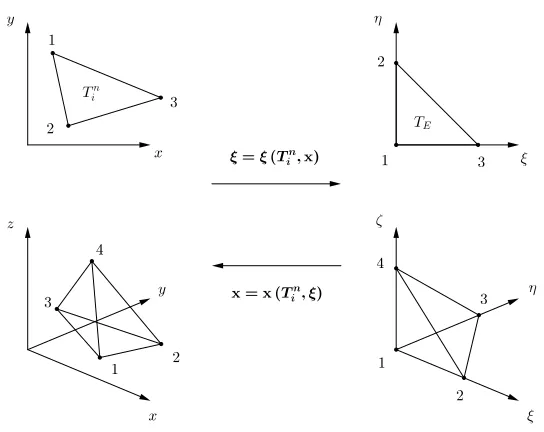
Since we are dealing with a moving computational domain where the mesh
configuration continuously changes in time, it is more convenient to map the
physical element
T
i
n
to a reference element
TE
via a
local
reference coordinate
system
ξ
−
η
−
ζ
. The spatial reference element
TE
is the unit tetrahedron
(or the unit triangle in 2D) shown in Figure 2.1 and is defined by the nodes
ξ
e,1
= (
ξe,1
, ηe,1, ζe,1
) = (0
,
0
,
0),
ξ
e,2
= (
ξe,2, ηe,2, ζe,2
) = (1
,
0
,
0),
ξ
e,3
=
(
ξe,3, ηe,3, ζe,3
) = (0
,
1
,
0) and
ξ
e,4
= (
ξe,4
, ηe,4
, ζe,4
) = (0
,
0
,
1), where
ξ
=
2.2 Polynomial WENO reconstruction
position vector
x
= (
x, y, z
) is defined in the physical system. Let furthermore
X
k,i
n
= (
X
n
k,i
, Y
n
k,i
, Z
n
k,i
) be the vector of physical spatial coordinates of the
k
-th
vertex of element
T
n
i
. Then the linear mapping from
T
i
n
to
Te
is given by
x
=
X
1,i
n
+
X
n
2,i
−
X
n
1,i
ξ
+
X
3,i
n
−
X
n
1,i
η
+
X
4,i
n
−
X
n
1,i
ζ.
(2.3)
When
d
= 2 the same transformation applies for the coordinates
x
and
y
,
setting
ζ
= 0. The vertices of
T
n
i
are given a connectivity
C
with a
counter-clockwise convention, as illustrated in Figure 2.1, hence
C
=
(
(1
,
2
,
3)
,
if
d
= 2
,
(1
,
2
,
3
,
4)
,
if
d
= 3
.
(2.4)
The piecewise constant cell averages, which represent the data that are stored
and evolved in time within a finite volume scheme, are defined at each time
level
t
n
within the control volume
T
i
n
as
Q
i
n
=
1
|
T
n
i
|
Z
T
n
i
Q
(
x
, t
n
)
d
x
,
(2.5)
with
|
T
i
n
|
denoting the volume of element
T
i
n
. The key point of any finite
volume schemes is the so-called numerical flux function, which computes the
fluxes across the boundaries of the control volume
T
n
i
. According to Godunov’s
idea [134], the numerical flux function can be defined by solving local Riemann
problems at the interfaces of the control volumes. If we limit us to use only the
values given by (2.5) to evaluate the numerical fluxes, we obtain a first order
accurate numerical scheme. In order to construct higher order finite volume
schemes we need to improve the order of accuracy of the solution employed
for the computation of the numerical flux function. In the next Section 2.2
a WENO reconstruction technique is described and used to obtain piecewise
higher order polynomials
w
h
(
x
, t
n
) from the known cell averages
Q
i
n
. High
order of accuracy in time is achieved later in Section 2.3 by applying a
lo-cal space-time Galerkin predictor method to the reconstruction polynomials
w
h
(
x
, t
n
).
2.2 Polynomial WENO reconstruction
The WENO reconstruction operator produces piecewise polynomials
w
h
(
x
, t
n
)
Figure 2.1:
Spatial mapping from the physical element
T
n
i
defined with
x
to
the unit reference element
TE
in
ξ
for triangles (top) and
tetra-hedra (bottom). Vertices are numbered according to the local
connectivity
C
given by (2.4).
known cell averages within a so-called
reconstruction stencil
S
s
i
, which is
com-posed of an appropriate neighborhood of element
T
n
i
and contains a prescribed
total number
ne
of elements which depends on the order
M
of the
polyno-mial. We do not use the original
pointwise
WENO method first introduced by
Shu et al. [144, 146, 249], but we adopt the
polynomial
formulation proposed
2.2 Polynomial WENO reconstruction
In [29, 151, 186] it has been shown that the total number of elements
ne
must
be greater than the smallest number
M
needed to reach the formal order of
accuracy
M
+ 1. As suggested in [101, 102] we normally take
ne
=
d
· M, with
M
=
d
Y
k=1
(
M
+
k
)
d
!
.
(2.6)
According to [102] we always use seven (1
≤
s
≤
7) and nine (1
≤
s
≤
9)
reconstruction stencils in two and three space dimensions, respectively.
Specif-ically,
s
= 1 denotes the central stencil, while one half of the remaining stencils
are the so-called forward stencils and the others are the backward
reconstruc-tion stencils, as depicted in Figures 2.2-2.3. For reconstrucreconstruc-tion, each element
T
i
n
and its surrounding elements are first mapped to the reference coordinate
system
ξ
−
η
−
ζ
using the mapping (2.3) in order to avoid ill-conditioned
re-construction matrices, see [4]. The three types of stencils (central, forward and
backward) are then obtained by a recursive algorithm which adds recursively
neighbor elements to the stencil until the prescribed number
ne
is reached.
Therefore:
•
for the central stencil (
s
= 1), we first add the Neumann neighbors of
T
n
i
(i.e. the direct side neighbors surrounding element
T
i
n
) to the stencil,
and then recursively continue adding the neighbors of these neighbors,
until the desired total number of elements in the stencil
ne
is reached;
•
each of the three forward stencils (2
≤
s
≤
4 in 2D and 2
≤
s
≤
5 in 3D)
is filled with elements using the same recursive algorithm, but adding
only those elements whose barycenters are located in the corresponding
forward sector. On triangular meshes (
d
= 2) the three forward sectors
are spanned by a vertex of the triangle and the pair of vectors connecting
this vertex with the two vertices of the opposite edge, while for tetrahedra
(
d
= 3) the four forward stencils are defined by a vertex
k
of the
tetra-hedron
T
i
n
and the triplet of vectors connecting
k
to the three vertices of
the opposite face;
•
the three backward stencils (5
≤
s
≤
7 in 2D and 6
≤
s
≤
9 in 3D)
are constructed in the same way as the forward stencils. The associated
backward sectors cover the remaining part of
R
d
that has not been
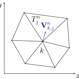
For the central stencil we use a simple Neumann-type neighbor search algorithm
that recursively adds direct face neighbors to the stencil, until the desired
num-ber
ne
is reached. For the remaining one-sided stencils we use a Voronoi-type
search algorithm, which fills the stencil starting from the vertex neighborhood
of the control volume and then using recursively vertex neighbors of stencil
elements. Figures 2.2-2.3 show the stencils used for the WENO reconstruction
technique on triangular and tetrahedral meshes, respectively.
Figure 2.2:
Two-dimensional WENO reconstruction stencils in the physical
(top row) and in the reference (bottom row) coordinate system
for
M
= 2, hence
ne
= 12: one central stencil (left), three forward
stencils (center) and three backward stencils (right).
Once the stencil search procedure has been carried out, each stencil contains
a total number of elements
ne
that depends on the reconstruction degree
M
given by (2.6), hence
S
s
i
=
n
e
[
j=1
T
m(j)
n
,
(2.7)
where 1
≤
j
≤
ne
is a local index which progressively counts the elements in
2.2 Polynomial WENO reconstruction
Figure 2.3:
Three-dimensional WENO reconstruction stencils in the physical
(top row) and in the reference (bottom row) coordinate system
for
M
= 2, hence
ne
= 30: one central stencil (left), four forward
stencils (center) and four backward stencils (right).
the global index of the element in
T
n
Ω
.
The high order reconstruction polynomial for each candidate stencil
S
s
i
for
element
T
n
i
is written in terms of the
orthogonal
Dubiner-type basis functions
ψl
(
ξ, η, ζ
) [72, 90, 149] on the reference element
Te
, i.e.
w
h
s
(
x
, t
n
) =
M
X
l=1
ψl
(
ξ
) ˆ
w
l,i
n,s
:=
ψl
(
ξ
) ˆ
w
n,s
l,i
,
(2.8)
where the mapping to the reference coordinate system is given by (2.3) and
ˆ
w
l,i
n,s
denote the
unknown
degrees of freedom (expansion coefficients) of the
reconstruction polynomial on stencil
S
s
i
for element
T
i
n
at time
t
n
. In the
rest of this manuscript we will use classical tensor index notation based on
the Einstein summation convention, which implies summation over two equal
indices. For a more details on the space basis functions
ψl
(
ξ
) we refer to Section
Integral conservation is required for the reconstruction on each element
T
j
n
of
the stencil
S
s
i
, yielding
1
|
T
n
j
|
Z
T
n
j
ψl
(
ξ
) ˆ
w
l,i
n,s
d
x
=
Q
j
n
,
∀
T
j
n
∈ S
i
s
.
(2.9)
Inserting the transformation (2.3) into the above expression (2.9), an
ana-lytical integration formula can be obtained that is a function of the physical
vertex coordinates
X
n
k,j
of the element. The resulting algebraic expressions
of the integrals appearing in (2.9) can be obtained for example at the aid of
a symbolic computer algebra system like MAPLE. Up to
M
= 3 we use the
aforementioned analytical integration, while for higher reconstruction degrees
the integrals in (2.9) are simply evaluated using Gaussian quadrature formulae
of suitable order, see [218] for details, since the analytical expressions become
too cumbersome. The reconstruction matrix, which is given by the integrals
of the linear system (2.9), depends on the geometry of the control volumes in
stencil
S
s
i
. Therefore, since in the Lagrangian framework the mesh is moving
in time, the reconstruction matrix can
not
be inverted and stored once and for
all during a pre-processing stage, like in the Eulerian case. As a consequence,
we assemble and solve the small reconstruction system (2.9) for each element
T
i
n
directly at the beginning of each time step
t
n
using optimized LAPACK
subroutines. This makes the ALE WENO reconstruction
computationally more
expensive
but at the same time also
much less memory consuming
compared
to the original Eulerian WENO algorithm presented in [101, 102], since no
re-construction matrices are stored.
While the mesh is moving in time, we always assume that the connectivity of
the mesh and therefore also the topology of each reconstruction stencil remains
constant in time. Therefore, the definition of the stencils
S
s
i
does
not
need to
be updated during the simulation. This is a very important simplification, since
the stencil search may be quite time consuming in multiple space dimensions
on unstructured meshes.
Since each stencil
S
s
i
is filled with a total number of
ne
=
d
· M
elements,
system (2.9) results in an overdetermined linear system that has to be solved
properly by either using a constrained least-squares technique (LSQ), see [102],
or a more sophisticated singular value decomposition (SVD) algorithm. The
use of the reference coordinate system ensures the matrix of the linear system
(2.9) to be reasonably well conditioned.
2.3 Local space-time Galerkin predictor on moving curved meshes
non-oscillatory, it must be
nonlinear
. Therefore a nonlinear formulation has
to be used for the final WENO reconstruction polynomial. We first measure
the
smoothness
of each reconstruction polynomial obtained on stencil
S
s
i
by a
so-called oscillation indicator
σ
s
[146],
σ
s
= Σ
lm
w
ˆ
l,i
n,s
w
ˆ
n,s
m,i
,
(2.10)
which is computed on the reference element using the (universal) oscillation
indicator matrix Σ
lm
, which, according to [102], is given by
Σ
lm
=
X
1
≤
α+β+γ
≤
M
Z
T
e
∂
α+β+γ
ψl
(
ξ, η, ζ
)
∂ξ
α
∂η
β
∂ζ
γ
·
∂
α+β+γ
ψm
(
ξ, η, ζ
)
∂ξ
α
∂η
β
∂ζ
γ
dξdηdζ.
(2.11)
In two space dimensions the above expression holds with
ζ
= 0 and
γ
= 0.
The nonlinearity is then introduced into the scheme by the WENO weights
ω
s
,
which read
˜
ω
s
=
λs
(
σ
s
+
)
r
,
ω
s
=
˜
ω
s
P
k
ω
˜
k
,
(2.12)
with the parameters
r
= 8 and
= 10
−
14
.
According to [102] the linear
weights are chosen as
λ1
= 10
5
for the central stencil and
λs
= 1 for the
remaining one-sided stencils. Formula (2.12) is intended to be read
componen-twise. For a WENO reconstruction based on characteristic variables see [101].
A weighted nonlinear combination of the reconstruction polynomials obtained
on each candidate stencil
S
s
i
yields the final WENO reconstruction polynomial
and its coefficients:
w
h
(
x
, t
n
) =
M
X
l=1
ψl
(
ξ
) ˆ
w
l,i,
n
with
w
ˆ
l,i
n
=
X
s
ω
s
w
ˆ
l,i
n,s
.
(2.13)
Within this work we may also refer to an
M-th order accurate reconstruction
polynomial with the notation
P
M
, meaning that the reconstruction procedure
has been carried out using polynomial of degree
M
.
2.3 Local space-time Galerkin predictor on moving curved
meshes
The reconstructed polynomials
w
h
(
x
, t
n
) computed at the current time
t
n
are
then
evolved
during one time step, i.e. up to time
t
n+1
,
locally
within each
obtains piecewise space-time polynomials of degree
M
, denoted by
q
h
(
x
, t
).
This allows the scheme to achieve also high order of accuracy in time. Such an
element-local time-evolution procedure has also been used within the MUSCL
scheme of van Leer [241] and the original ENO scheme of Harten et al. [138],
who called this element-local predictor with initial data
w
h
(
x
, t
n
) the solution
of a Cauchy problem
in the small
, since no information from neighbor elements
is used. The coupling with the neighbor elements occurs only later in the
fi-nal one-step finite volume scheme (see Section 2.5). While the origifi-nal ENO
scheme of Harten et al. uses a higher order Taylor series in time together with
the
strong
differential form of the PDE to substitute time–derivatives with
space derivatives (the so–called Cauchy–Kovalewski or Lax–Wendroff
proce-dure [159]), here a
weak
formulation of the governing PDE (2.1) in space-time
is derived (see Eqn. 2.28 below). The resulting method does not require the
computation of higher order derivatives, but just pointwise evaluations of the
fluxes, source terms and non-conservative products appearing in the PDE. This
approach has first been developed for the Eulerian framework on fixed grids
in [95, 98, 99, 141] and here we extend it to moving unstructured meshes in
multiple space dimensions.
Let
x
= (
x, y, z
) and
ξ
= (
ξ, η, ζ
) be the spatial coordinate vectors defined in
the physical and in the reference system, respectively, and let
x
˜
= (
x, y, z, t
)
and
ξ
˜
= (
ξ, η, ζ, τ
) be the corresponding space-time coordinate vectors. Let
furthermore
θl
=
θl
(
ξ
˜
) =
θl
(
ξ, η, ζ, τ
) be a space-time basis function defined
by the Lagrange interpolation polynomials passing through a set of space-time
nodes
ξ
˜
m
= (
ξm, ηm, ζm, τm
). For the Discontinuous Galerkin (DG)
predic-tor, illustrated in Section 2.3.2, the space-time nodes are defined by the tensor
product of the spatial nodes of classical conforming high order finite elements
and the Gauss-Legendre quadrature points in time, while in the Continuous
Galerkin (CG) approach the coordinates of the space-time points are chosen
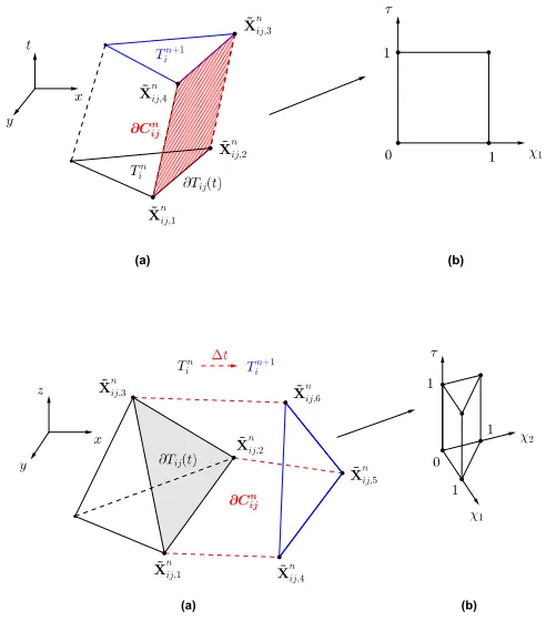
according to [94]. The two-dimensional reference and physical space-time
el-ement configuration as well as the associated space-time nodes for the case
M
= 2 are depicted in Figures 2.4 and 2.5 for the CG and the DG predictor
algorithm, respectively. More details are also given in Section A.2 of Appendix
A.
Since the Lagrange interpolation polynomials define a
nodal
basis, the functions
θl
satisfy the following interpolation property:
θl
(
ξ
˜
m
) =
δlm,
(2.14)
where
δlm
denotes the usual Kronecker symbol. Following [95] the local solution
2.3 Local space-time Galerkin predictor on moving curved meshes
product
P
h
=
B
(
q
h
)
· ∇
q
h
are approximated within the space-time element
Ti
(
t
)
×
[
t
n
;
t
n+1
] with
q
h
=
q
h
(
ξ
˜
) =
θl
(
ξ
˜
)
q
b
l,i,
F
h
=
F
h
(
ξ
˜
) =
θl
(
ξ
˜
)
F
b
l,i,
S
h
=
S
h
(
ξ
˜
) =
θl
(
ξ
˜
)
S
b
l,i,
P
h
=
P
h
(
ξ
˜
) =
θl
(
ξ
˜
)
P
b
l,i.
(2.15)
Because of the interpolation property (2.14) we evaluate the degrees of freedom
for
F
h
,
S
h
and
P
h
in a
pointwise
manner from
q
h
as
b
F
l,i
=
F
(
q
b
l,i
)
,
S
b
l,i
=
S
(
b
q
l,i
)
,
P
b
l,i
=
P
(
q
b
l,i,
∇
b
q
l,i
)
,
∇
q
b
l,i
=
∇
θm
(
ξ
˜
l
)
q
b
m,i.
(2.16)
The degrees of freedom
∇
q
b
l,i
represent the gradient of
q
h
in node
ξ
˜
l
.
An
isoparametric
approach is used, where the mapping between the physical
space-time coordinate vector
˜
x
and the reference space-time coordinate vector
˜
ξ
is represented by the
same
basis functions
θl
used for the discrete solution
q
h
itself. Therefore
x
(
ξ
˜
) =
θl
(
ξ
˜
)
x
b
l,i,
t
(
ξ
˜
) =
θl
(
ξ
˜
)
b
tl,
(2.17)
where
b
x
l,i
= (
b
xl,i,
yl,i,
b
zl,i
b
) are the degrees of freedom of the spatial physical
coordinates of the moving space-time control volume, which are unknown, while
b
tl
denote the
known
degrees of freedom of the physical time at each space-time
node ˜
x
l,i
= (
b
xl,i,
b
yl,i,
zl,i,
b
b
tl
). The mapping in time is linear and simply reads
t
=
tn
+
τ
∆
t,
τ
=
t
−
t
n
∆
t
,
⇒
b
tl
=
tn
+
τl
∆
t,
(2.18)
where
t
n
represents the current time and ∆
t
is the current time step, which
is computed under a classical Courant-Friedrichs-Levy number (CFL) stability
condition, i.e.
∆
t
= CFL min
T
n
i
di
|
λmax,i
|
,
∀
T
n
i
∈
Ω
n
,
(2.19)
with
di
denoting the insphere or incircle diameter of element
T
i
n
and
|
λmax,i
|
corresponding to the maximum absolute value of the eigenvalues computed
from the solution
Q
i
n
in
T
i
n
. In multiple space dimensions, the CFL condition
must satisfy the inequality CFL
≤
1
d
if one-dimensional Riemann solvers are
The Jacobian of the transformation from the physical space-time element to
the reference space-time element reads
Jst
=
∂
˜
x
∂
ξ
˜
=
xξ
xη
xζ
xτ
yξ
yη
yζ
yτ
zξ
zη
zζ
zτ
0
0
0
∆
t
(2.20)
and its inverse is given by
J
st
−
1
=
∂
ξ
˜
∂
x
˜
=
ξx
ξy
ξz
ξt
ηx
ηy
ηz
ηt
ζx
ζy
ζz
ζt
0
0
0
1
∆t
.
(2.21)
We point out that in the Jacobian matrix
tξ
=
tη
=
tζ
= 0 and
tτ
= ∆
t
, as can
be easily derived from the time mapping (2.18).
In the following we introduce the notation adopted for the nabla operator
∇
in the reference space
ξ
= (
ξ, η, ζ
) and in the physical space
x
= (
x, y, z
):
∇
ξ
=
∂
∂ξ
∂
∂η
∂
∂ζ
,
∇
=
∂
∂x
∂
∂y
∂
∂z
=
ξx
ηx
ζx
ξy
ηy
ζy
ξz
ηz
ζz
∂
∂ξ
∂
∂η
∂
∂ζ
=
∂
ξ
∂
x
T
∇
ξ
.