Simulating and validating the effects of slope frost heaving on canal bed saturated soil using coupled heat-moisture-deformation model

Simulating and validating the effects of slope frost heaving on

canal bed saturated soil using coupled heat-moisture-deformation

model

Wang Enliang

1,2,3

_,

_{Fu Qiang}

1,2,3*

_,

_{Liu Xingchao}

1

_,

_{Li Tianxiao}

1,2,3

_,

_{Li Jinling}

1

(1. School of Water Conservancy and Civil Engineering, Northeast Agricultural University, Harbin 150030, China;

2. Heilongjiang Provincial Collaborative Innovation Center of Grain Production Capacity Improvement, Northeast Agricultural University, Harbin 150030, China; 3. Key Laboratory of High Efficient Utilization of Agricultural Water Resource of Ministry of Agriculture,

Northeast Agricultural University, Harbin 150030, China)

Abstract: The lining canals in seasonal frozen soil areas can be severely damaged by frost heaving. The freezing and thawing contributes to the continual change of the temperature field and moisture field beneath lining canal, which will seriously affect the safe operation of the canal. In order to study the frost heaving damage mechanism of lining canal and to solve the associated engineering problems, the permafrost body was regarded as an elastomer, and a three-field, coupled, partial differential equation describing the temperature, moisture and deformation fields for a saturated two-dimensional canal bed was derived and established based on the Harlan model. The coupling equations were discretized using the finite element method in space and the finite difference method in time. The parameters were simplified appropriately based on compliance with the actual conditions and were simulated using finite element software. The results of a sample simulation showed that the simulated results and test results were basically consistent with variation laws, which proved the correctness of the numerical simulation theory and solution methods and the reliability of the calculation. The model can simulate the water, heat and deformation issues in the side slope of saturated canal bed soil in a seasonally frozen area and forecast freezing damage in the canals.

Keywords: seasonally frozen area, canal, soil of the side slope, coupling of water, heat and deformation, model DOI: 10.3965/j.ijabe.20171002.2551

Citation: Wang E L, Fu Q, Liu X C, Li T X, Li J L. Simulating and validating the effects of slope frost heaving on canal bed saturated soil using coupled heat-moisture-deformation model. Int J Agric & Biol Eng, 2017; 10(2): 184–193.

1 Introduction

The reality of the increasingly scarcity of global water resources has made water-saving research an important issue. Frost heaving problems commonly occur in canals in seasonal frost areas and have seriously affected

Received date: 2016-04-25 Accepted date: 2017-03-02 Biographies: Wang Enliang, PhD, Professor, research interests: frost damage prevention and treatment of frozen soil engineering and hydraulic structures, Email: [email protected]; Liu Xingchao, Graduate student, research interest: frost damage prevention and treatment of frozen soil engineering and hydraulic structures, Email: [email protected]; Li Tianxiao, PhD candidate, research interests: optimization and utilization of agricultural water and soil resources andsystemanalysis, Email:

the safe operation of canals. Scholars both at home and abroad have conducted many studies on frost heaving

damage to canals[1-9]_{. The direct cause of frost damage}

in canal linings is frost heaving of the canal base soil[10].

The coupled water, heat and force issues are the key problems in permafrost research and are also at the

March, 2017 Wang E L, et al. Simulating the slope frost heaving on saturated soil using HMD model Vol. 10 No.2 185

forefront of international research in this area[11]_.

Throughout the history of permafrost theory development,

many scholars have proposed various models. Harlan[12]

first proposed water-thermal coupling concepts in 1973 and established a water-heat coupling model in accordance with the principles of unfrozen water dynamics and energy conservation, which made him the founder of modern coupling analysis. In 1978, Taylor et

al.[13] and other scholars proposed the finite difference

scheme to facilitate solutions based on the Harlan model.

In 1987, based on this scheme, Shen et al.[14] proposed

three-field coupling issues, including water (moisture field), heat (temperature field), and force (stress field), based on the Harlan hydrodynamic model and provided a

simplified coupling model. In 1989, An[15] _{and other}

scholars conducted a preliminary analysis of the water-heat coupling problems in the soil freezing process

and provided examples. Lai et al.[16] _{first derived the}

mathematical mechanical model and governing differential equations of the coupled problem of temperature-seepage-stress fields with phase change from heat transfer theory, seepage theory and frozen soil

mechanics. Masters et al.[17] investigated the coupling

rule of soil deformation, fluid temperature and pore pressure by taking the temperature, pore pressure and soil

displacement as initial unknown quantities. Li et al.[18]

established a heat-moisture-deformation coupling model based on the theory of equilibrium, continuity and energy principles of a multi-phase porous medium. The force interactions between the soil skeleton and ice particles and the energy jump behaviours during the phase change between ice and water were considered in this model.

Gens et al.[19] established a new mechanical model that

encompasses frozen and unfrozen behaviour within a unified, effective-stress-based framework. In recent years, studies of the three coupled field issues of frozen ground water, heat and force have been rich. With the development of computer technology, more theoretical studies have focused on the coupling mechanisms of permafrost water, heat and forces and the application of

the finite element method[20-23].

Canal lining damage occurs mainly because of large uneven displacements of the lining body that result from

frost heaving of canal bed soil. The lining is generally characterized by its small size, light weight and small binding force; these factors make the heaving force difficult to control and thus allow it to cause damage. Therefore, the displacement caused by frost heaving was

chosen as the main control target[24]. Currently, there

are few studies on the interactions among water, heat and the deformation of slope soil in canals. In this study the side slope of the canal with the most unfavourable working conditions were selected as the analytical object. A model coupling water, heat and deformation of the saturated soil in the canal bed was created based on the viscous flow of liquid water in porous media, the principles of thermal equilibrium, and the foundation of moisture migration theory and frost heave mechanisms, which can provide a basis for frost heave forecasts of the canal base and for the anti-freezing design.

2 Mathematical model

2.1 Basic assumptions

To facilitate solving the mathematical model, the following basic assumptions were adopted:

1) The soil particles are incompressible and do not deform during the freezing and thawing processes. Only volume changes caused by frost heaving of the soil moisture are considered.

2) Only liquid water migration is considered; gaseous water migration is ignored.

3) Heat conduction is considered; vapour convection is ignored.

4) The soil is a homogeneous, isotropic elastic material, and the positive and water anisotropy coefficients, as well as the thermal conductivity in the thawing and permafrost soil, are constants.

5) The impacts of soil salinity are ignored. 6) The pore water seepage obeys Darcy’s Law. 7) The impacts of external loads on the canal lining structure are excluded.

2.2 Basic equations

2.2.1 Heat transfer equation

Based on the above assumptions, the frost heaving

to the studies of Taylor and others on freezing and thawing processes, the heat conduction term is 2 to 3 orders of magnitude greater than the convective terms. Therefore, if we ignore the influence of convection, the two-dimensional steady-state heat conduction equation at

a given time is as follows[25]:

t L z T z x T x t T

C i

i _∂

∂ + ⎟ ⎠ ⎞ ⎜ ⎝ ⎛

∂ ∂ ∂

∂ + ⎟ ⎠ ⎞ ⎜ ⎝ ⎛

∂ ∂ ∂

∂ = ∂

∂ _{λ λ ρ} θ ₍₁₎

where, C is the soil volumetric heat capacity, J/(m3·°C);

λ is the thermal conductivity, J/(m·s·°C); T is the

temperature, °C; t is time, s; x is the horizontal coordinate,

m; z is the vertical coordinate, m; L is the latent heat,

334.7 kJ/kg; θw and θi are the moisture and ice contents,

respectively, %; ρi is the ice density, kg/m3.

The solution of the heat conduction equation should satisfy the boundary condition T(L, t) = TL, where L is the

boundary of the freezing problem. 2.2.2 Water field equation

The moisture migration equation inside the saturated

or unsaturated soil can be expressed as follows[15]:

⎥⎦ ⎤ ⎢⎣ ⎡

∂ ∂ ∂

∂ + ⎥⎦ ⎤ ⎢⎣ ⎡

∂ ∂ ∂

∂ = ∂ ∂ + ∂ ∂

z K z x K x t t

i

w i

w θ ψ ψ

ρ ρ

θ ₍₂₎

The supplemental equation is

G Pw+ =

ψ (3)

From the rigid pore saturated soil, we obtain

nw+ni=n (4)

where, ρw and ρi are the densities of water and ice,

respectively, kg/m3; K is the hydraulic conductivity

coefficient, cm/s; ψ is the soil water potential, Pa; Pw is

water pressure, Pa; G is the gravitational potential, Pa;

and nw, ni, and n are the volumetric water content,

volumetric ice content and soil porosity, respectively, %. The gravity potential impact of water flow in the frozen layer is very small and can be ignored, and we can then obtain the following water field equation from Equations (2) and (3):

⎥⎦ ⎤ ⎢⎣ ⎡

∂ ∂ ∂

∂ + ⎥⎦ ⎤ ⎢⎣ ⎡

∂ ∂ ∂

∂ = ∂ ∂ + ∂ ∂

z P K z x P K x t t

w w

i

w i

w θ

ρ ρ

θ ₍₅₎

Substituting Equation (5) into Equation (1) and considering the moisture content of the freezing process

as a function of temperature T, then Equation (6) can be

obtained:

θ θ

∂ ₌∂ ∂

∂ ∂ ∂

w w T

t T t (6)

The equation used to describe the effects of stress in the soil is

0

ln( )

ρw_w −ρi_i =

P P T

L

T (7)

In this calculation, when the soil is considered to be

unloaded and the salt content is small and uniform, Pi=0,

and Equation (7) becomes

0

ln( )

ρ

=

w w

T

P L

T (8)

where, T0 _{is the water freezing temperature, °C.}

2.2.3 Deformation field equation

When the in situ moisture is frozen in the canal bed, the frost heaving stress incurred in a certain time period is

0 1

d( )

0.09 d

θ θ

ε = − u

T (9)

where, ε1 is the in situ stress caused by frost heaving;θ0 is

the original water content; θu _{is the unfrozen water}

content; and T is the temperature at any time.

In the open system, the amount of frost heaving caused by the input of outside water per unit time is

2

d[ ( ) ]

1.09 d

θ

ε = q t − u

h

(10)

In this equation, ε2 _{is the frost heaving stress caused}

by the amount of outside water added to the system, and h

is the original height of a certain point in the canal.

Then, the total frost heaving stressεis

1 2

ε ε= +ε (11) We can then calculate the total frost heaving of the canal surface based on the frost heaving stress.

2.2.4 Coupling of the equations

From Equations (1)-(11), we can obtain the following equations:

) ( ) (

z T z x T x t T C

∂ ∂ ∂

∂ + ∂ ∂ ∂

∂ = ∂

∂ _{λ λ}

(12)

T L C

C w

w _∂ ∂ +

= ρ θ

(13)

T K L2_ρw2 /

λ

λ= + (14)

where, C and λ are the heat capacity and heat

March, 2017 Wang E L, et al. Simulating the slope frost heaving on saturated soil using HMD model Vol. 10 No.2 187

,

( ) / 2,

, + + − − ⎧ > ⎪ =_⎨ + ≤ ≤ ⎪ _< ⎩ P b P P C T T

C C C T T T

C T T

(15) ⎪ ⎩ ⎪ ⎨ ⎧ < ≤ ≤ + > = − − + + P P b P T T T T T T T , , 2 / ) ( , λ λ λ λ λ

(16) ⎪ ⎩ ⎪ ⎨ ⎧ < ≤ ≤ + > = − − + + P P b P T T K T T T K K T T K K , , 2 / ) ( , (17)

In Equations (15)-(17), Tp _and Tb _{are the upper and}

lower temperature boundaries, respectively, of the severe phase transition zone.

Equations (1) to (17) are not convergent, which means that they cannot be solved analytically. Therefore, numerical methods must be used. Meanwhile, a relationship between the unfrozen water content and temperature is also needed:

( )

θ_w = f T (18) The migration of unfrozen water in the frozen soil occurs under the action of an uneven force (temperature gradient or potential gradient). Tests have proven that after the soil freezes, not all the liquid water is converted into solid ice; there is always some liquid water surrounding the particles at a certain negative temperature. Additionally, there is always a particular dynamic equilibrium relation between the unfrozen water content

of the frozen soil and the negative temperature[26],

described as follows:

b

w aT

θ = (19)

b T

a=θ_{1 2} (20)

2 1 2 1 ln ln ln ln T T b − −

= θ θ (21)

In Equations (19)-(21), T1 and T2 are the absolute

values of the negative temperature for the corresponding

unfrozen water contents of θ1andθ2, respectively; a and

b are constants related to the soil properties.

The moisture migration of the frozen soil complies

with Darcy's law[14]_{, namely,}

d

d ( )

d

ψ θ

=

W K

z (22)

where, dW is the moisture migration velocity or inflow

speed (cm/s); K(θ) is the moisture migration factor, i.e.,

the hydraulic conductivity coefficient; and d

d

ψ

z is the

soil water potential gradient, which is the driving force for migration and is directly reflected in the temperature gradient. Initial conditions: ) , ( ) 0 , ,

(x z 1 x z

w ϕ

θ = (23)

) , ( ) 0 , ,

(x z ₂ x z

T =ϕ

(24)

Boundary conditions: ) ( ) , 0 ,

(x t F1 t

T = (25)

) ( ) , ,

(x L1 t F2 t

T = (26)

) , ( ) , , 0 (

3 t z

F x t z T ₌ ∂ ∂ (27) ) , ( ) , , ( 4

2 _{F t z}

x t z L T ₌ ∂ ∂ (28)

Given the initial conditions, the boundary conditions and the relationship between the unfrozen water content and temperature, the equation is a closed nonlinear problem, which can be solved numerically.

2.2.5 Model solving

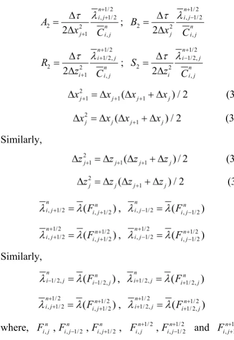
There isn’t analytical solution for nonlinear problems, this problem can be solved using a combined finite element and finite difference method, where the finite element method is used for the spatial aspects, and the finite difference method is used for the temporal component. Through discretization of the above mentioned heat conduction equation in accordance with the conservation law of the variable coefficient equation difference scheme, we obtained the following results:

) ( ) ( ) ( ) ( , 1 , 1 , , 1 1 2 / 1 1 , 2 / 1 , 1 2 / 1 , 2 / 1 1 , 1 , 2 / 1 , n j i n j i n j i n j i n j i n j i n j i n j i n j i n j i T T S T T R T T B T T A T T − + + − + + + + + − − − + − − − = − (29) ) ( ) ( ) ( ) ( 2 / 1 1 , 2 / 1 , 2 2 / 1 , 2 / 1 1 , 2 1 , 1 1 , 2 1 , 1 , 1 2 2 / 1 , 1 , + − + + + + + − + + + + + + − − − + − − − = − n j i n j i n j i n j i n j i n j i n j i n j i n j i n j i T T B T T A T T S T T R T T (30) where, n j i n j i j C x A , 2 / 1 , 2 1 1 ₂ + + Δ Δ

= τ λ ; _n

j i n j i j C x B , 2 / 1 , 2 1 ₂ − Δ Δ

= τ λ

1/2,

1 2

1 ,

2

τ λ+

+ Δ = Δ n i j n

i i j

R

z _C ;

1/2,

1 2

,

2

τ λ−

Δ = Δ n i j n

i i j

S

n j i n j i j C x A , 2 / 1 2 / 1 , 2 1 2 ₂ + + + Δ Δ

= τ λ ; _n

j i n j i j C x B , 2 / 1 2 / 1 , 2 2 ₂ + − Δ Δ

= τ λ

1/2 1/2,

2 2

1 ,

2

τ λ++

+ Δ = Δ n i j n

i i j

R

z _C ;

1/2 1/2,

2 2

,

2

τ λ−+

Δ = Δ n i j n

i i j

S

z _C

2

1 1( 1 ) / 2

+ + +

Δx_j = Δx_j Δx_j + Δx_j (31)

2

1

( ₊ ) / 2

Δ = Δ Δx_j x_j x_j + Δx_j (32)

Similarly, 2 / ) ( ₁ 1 2

1 j j j

j z z z

z =Δ Δ +Δ

Δ _{+ + +} (33)

2

1

( ₊ ) / 2

Δ = Δ Δzj zj zj + Δzj (34)

, 1/2 ( _{, 1/2})

λ + =λ ₊

n _n

i j F_{i j} , λ, −1/2=λ( _{, −1/2})

n _n

i j F_{i j}

1/2 _1/2 , 1/2 ( _{, 1/2})

λ + λ +

+ = ₊

n _n

i j F_{i j} ,

1/2 _1/2 , 1/2 ( _{, 1/2})

λ + λ +

− = ₋

n _n

i j F_{i j}

Similarly,

) ( 1/2, ,

2 /

1 _in _j

n j i− =λ F₋

λ , 1/2, ( 1/2, )

n j i n

j i+ =λ F₊

λ

)

( 1/2

2 / 1 , 2 / 1 2 / 1 , +₊ +

+ = _in_j

n j

i λ F

λ , ( 1/2)

, 2 / 1 2 / 1 , 2 /

1 ₊+

+

+ = _in _j

n j

i λ F

λ

where, n

j i

F_, , n

j i

F_,−1/2, n j i

F_,+1/2, 1/2 ,

+

n j i

F , 1/2

2 / 1 , + − n j i

F and 1/2

2 / 1 , + + n j i F

are the calculated temperature values on the right hand side of the difference equation, which can be expressed as

) ( _, , n j i n j

i F T

F = , ( 1/2)

2 / 1 , 2 / 1 2 / 1 , + + +

+ = inj

n j

i F T

F

similarly, we can obtain the expressions of n

j i F_,−1/2,

n j i

F_,+1/2, 1/2 ,

+

n j i

F and 1/2

2 / 1 , + − n j i F .

To simplify the calculation process, this study uses an equidistant grid, and the step size is equal in the x and z

directions, as follows: Δxj+1=Δxj ; Δzi+1=Δzi ;

h z

x=Δ =

Δ ; and order _n

j i C

h2 ,

2

τ

γ = Δ . Then, in the above

equation,

n j i A₁=

γ

λ

,+1/2;

n j i B₁=

γ

λ

,−1/2

1/2, 1=γ λ+

n

i j

R ; ₁=γ λ−1/2,

n

i j

S

1/2 , 1/2 2 γ λ

+ +

= ni j

A ; ₂ ,1/12/2

+ −

= nij

B

γ

λ

1/2 1/2, 2 γ λ

+ +

= in j

R ; ₂ γ λ 1/2,1/2

+ −

= ni j

S

From Equation (29), we obtain

n j i n j i n j i n j i n j i n j i T R T S R T S T A T B A T B , 1 1 , 1 1 , 1 1 2 / 1 1 , 1 2 / 1 , 1 1 2 / 1 1 , 1 ) 1 ( ) 1 ( + − + + + + − + − − + = − + + + − (35)

From Equation (30), we obtain

2 / 1 1 , 2 2 / 1 , 2 2 2 / 1 1 , 2 1 , 1 2 1 , 2 2 1 , 1 2 ) 1 ( ) 1 ( + + + + − + + + + − + − − + = − + + + − n j i n j i n j i n j i n j i n j i T A T B A T B T R T S R T S (36)

The coefficient matrix of the differential Equations (35) and (36) is mainly a tridiagonal coefficient matrix. We can use the chasing method to solve the unknown temperature values at each time layer. Then, we can determine the new boundary conditions, based on a real-time temperature value solution, to solve for the water distribution and total frost heaving value of the canal slope surface.

3 Model verification

3.1 Model test introduction

The “North Conveyance” Wubei section canal project of the Heilong River was chosen as a case study. The actual situation of the pilot project was combined with the field test section as a prototype to conduct the indoor model test. By simulating the natural frost and melting process with decreasing and increasing temperatures, we can study the damage conditions of protective prefabricated concrete slope panels in response to freeze-thaw cycles to provide the necessary data and references for further numerical simulation. The model profile and cross-section observations are shown in Figure 1.

Figure 1 Model profile of prefabricated concrete slope protective panel

March, 2017 Wang E L, et al. Simulating the slope frost heaving on saturated soil using HMD model Vol. 10 No.2 189

stabilization phase (see Figure 2). To simulate the underlying warm soil layer temperature of the natural soil, the floor temperature was controlled after the test began in accordance with the test experience, and the temperature was set at 3.0°C.

Figure 2 Testing temperature control process curve 3.2 Comparative analysis of numerical simulation and experimental results

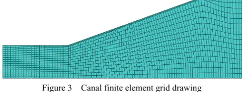
To better compare the calculation results with the indoor model test results, this paper uses the ABAQUS software to simulate the changing process of freezing and thawing in the canal’s temperature field, conducts a comparative analysis with the indoor model test results, and compares the calculation results of the water field and deformation field. Numerical simulation of the finite element model is shown in Figure 3.

Figure 3 Canal finite element grid drawing

3.2.1 Initial conditions and calculation parameters 1) Initial conditions: The initial boundary conditions are important factors that affect the temperature field. Boundary conditions can be mainly divided into three categories.

The first category is known as the temperature boundary condition, namely, the temperature value or temperature function on the boundary is given explicitly and can be expressed by the following formula:

Boundary= ( , )

T f r t (37)

In the second category, also known as the heat flux

boundary condition, the given heat flux of a certain area can be expressed by the following formula:

Boundary _{( , )}

λ∂

= =

∂

T

q q r t

n (38)

The third category, known as the convective heat transfer boundary condition, can be expressed by the following formula, given the changes of ambient fluid

temperature T* _{with time and the convective heat transfer}

coefficient:

) (

n Boundary

*

Boundary _{BT T}

T

− = ∂ ∂

−λ (39)

This study adopted the thermal boundary condition, which is widely used in engineering. The upper boundary had a convective boundary condition, for which the temperature control process line is the ambient temperature control curve shown in Figure 2. The vertical temperature on the two sides exhibited a heat flux boundary condition, where the heat flux was zero; the bottom line exhibited a constant temperature boundary condition, and the temperature was controlled to be 3.0°C.

2) Calculation parameters: The latent heat of a phase change is only relevant when the phase change occurs. The phase change interval of this simulation is taken to be from –0.3°C to 0.01°C; the latent heat of the phase change in the soil is 334 700 J/kg; the convective heat

transfer coefficient is 4.74 W/m2·°C; and the material

calculation parameters are shown in Table 1.

Table 1 Calculation parameters of the model

Material Parameters Positive temperature Negative temperature

Soil body

ρ 1940.00 1940.00

C 1174.70 1585.90

λ 1.54 1.83

Prefabricated concrete slab

ρ 2400.00 2400.00

C 840.00 840.00

λ 1.86 1.86

Sand gravel cushion

ρ 1800.00 1800.00

C 920.00 920.00

λ 1.86 1.86

Note: ρ is density, kg/m3_{; C is heat capacity, J/(kg·°C); λ is thermal conductivity,}

J/(m·s·°C).

temperature field changes obtained from the experiment. The change trend of the simulated temperature field is largely the same as the temperature change trend in the results of the simulated experiments, namely, there was a unidirectional freeze process but a two-way thawing process, which is in accordance with the previous

research results[15]_{. However, because the laboratory}

test conditions cannot be simulated completely, as there were some uncontrollable factors, there will always be some differences between the two.

3.2.3 Comparative analysis of the water field

A comparative analysis of the water field at the top position of the canal after the test was finished is shown in Figure 5.

a. Simulated temperature diagram at the beginning of the test b. Actual tested temperature diagram at the beginning of the test

c. Simulated temperature diagram at the deepest frost d. Actual tested temperature diagram at the deepest frost

e. Simulated temperature diagram at the end of the test f. Actual tested temperature diagram at the end of the test Figure 4 Comparative analysis of the temperature fields

a. Simulated water content diagram at the end of the test b. Actual tested water content diagram at the end of the test Figure 5 Water content diagram during the freeze-thaw process at the canal top

As shown in Figure 5, the trends in the changes in the numerically simulated water field and test results are roughly the same, water distribution present that the top is big and the underside is small in the vertical direction.

March, 2017 Wang E L, et al. Simulating the slope frost heaving on saturated soil using HMD model Vol. 10 No.2 191

the soil, and the temperature gradient at the top of the canal is greater than the temperature gradient at the lower portion. Therefore, the migration is obviously closer to the top of the canal, which thus gives the water content in the upper canal bed soil a certain advantage over the lower soil water content before freezing. During the melting process, the water infiltration decreases the moisture content, but this moisture content remains greater than the initial ones. Thus, it can be concluded

that the temperature gradient is the direct driving force for moisture migration. The unfrozen moisture migrates along the direction of lower temperatures due to the temperature gradient effect, and the larger the temperature gradient is, the greater the amount of migration. This result is consistent with literature [20]. 3.2.4 Comparative analysis of the deformation field

A comparative analysis of the canal slope’s deformation is shown in Figure 6.

a. Simulated deformation curve b. Actually tested deformation curve Figure 6 Deformation curves of freezing and thawing of the canal slope

The simulated deformation curve of the freeze- thawing process in Figure 6 is basically coincident with the tested deformation curve. The main difference is that there is no frost shrinking phenomenon at the beginning because the numerical simulation does not consider the expansion and contraction of soil particles. The maximum frost heave of canal slope appears in the 1/3 slope height and 1/2 slope height, which is

consistent with the calculated results of literature[27]_.

The agreement of the simulation results with the experimental results verifies that the frost heaving theory is equally applicable in the canal project and in the rationality of using the frozen quantity calculation formula. Through a freeze-thaw cycle, the heaving of the canal slope is greater than the thawing settlement, and the slope structure exhibits residual frost and uneven deformation, which results in uneven frost damage of the prefabricated concrete slope protection board. Photographs of some of the damage due to uneven frost accumulation are shown in Figure 7. The test results are coincident with the channel frost heaving damage phenomena.

Figure 7 Uneven frost damage phenomena

4 Conclusions

1) The interaction of the canal bed soil moisture field, temperature field and deformation field during the soil freezing process is an extremely complex issue involving thermal, physical, chemical and mechanical factors. Based on the Harlan model, the permafrost soil was considered as an elastomer to derive and establish a coupling equation for the temperature field, moisture field and deformation field in a saturated two- dimensional canal bed and proposed numerical solutions.

element software. The change laws of the simulated and experimental results are consistent, and the damage modes are consistent with the field surveys. These results show the correctness of the numerical simulation theory and solution methods as well as the reliability of the calculation results.

3) This study has considered the most unfavourable operating conditions, with the canal bed soil in a saturated state, but has ignored the effects of the pore volume. Due to the limitations of the test conditions, the more complex coupling relationship of the water, temperature and deformation in the canal bed’s unsaturated slope soil will require further study.

Acknowledgements

The authors are grateful for the financial support from the National Natural Science Foundation (51541901), Heilongjiang Province Natural Science Foundation (E201405), and Heilongjiang Province Post-Graduate Foundation (LBH-Z13031).

[References]

[1] Jay S, Jack H. Canal-Lining demonstration project year 10 final report. Department of the Interior, USA, 2002. [2] Herve P. Application of Geosynthetics in Irrigation and

Drainage Projects. International Commission on Irrigation and Drainage, New Delhi, India, 2004.

[3] Jiang H, Zheng Y. Mechanics models of frost heaving damage on composite lining trapezoidal canal with arc-bottom. International Journal of Applied Mathematics and Statistics, 2013; 41(11): 139–150.

[4] Shen X D, Zhang Y P, Wang L P. Stress analysis of frost heave for precast concrete panel lining trapezoidal cross-section channel. Transactions of the CSAE, 2012; 28(16): 80–85. (in Chinese)

[5] Li A G, Li H, Cheng Q H. Study on the prediction of frost heave in the bedsoil of canals. Water Resources & Water Engineering, 1993; 4(3): 17–23. (in Chinese)

[6] Li S Y, Lai Y M, Pei W S, Zhang S J, Zhong H. Moisture-temperature changes and freeze-thaw hazards on a canal in seasonally frozen regions. Natural Hazards, 2014; 72(2): 287–308.

[7] Wang Z Z, Li J L, Chen T, Guo L X, Yao R F. Mechanics models of frost-heaving damage of concrete lining

trapezoidal canal with arc-bottom. Transactions of the CSAE, 2008; 24(1): 18–23. (in Chinese)

[8] Wang E L, Li J L. Experimental study of the influence of freeze and thaw cycle on shear strength of concrete slope protection. Journal of Glaciology and Geocryology, 2012; 34(5): 1173–1178. (in Chinese)

[9] Li Z, Liu S H, Feng Y T, Liu K, Zhang C C. Numerical study on the effect of frost heave prevention with different canal lining structures in seasonally frozen ground regions. Cold Regions Science & Technology, 2013; 85(1): 242–249. [10] Liao Y, Liu J J, Chen S F. Research progress of damage mechanism of frost heave and anti-frost technique of concrete canal. Rock and Soil Mechanics, 2008; 29(S1): 211–214. (in Chinese)

[11] Zhu Z W, Ning J G, Ma W. Constitutive model and numerical analysis for the coupled problem of water, temperature and stress fields in the process of soil freeze-thaw. Engineering Mechanics, 2007; 24(5): 138–144, 137. (in Chinese)

[12] Harlan R L. Analysis of coupled heat-fluid transport in partially frozen soil. Water Resource Research, 1973; 9(5): 1314–1323.

[13] Taylor G S, Luthin J N. A model for coupled heat and moisture transfer during soil freezing. Canadian Geotechnical Journal, 1978; 15(4): 548–555.

[14] Shen M, Ladanyi B. Modelling of coupled heat, moisture and stress field in freezing soil. Cold Regions Science & Technology, 1987; 14(3): 237–246.

[15] An W D. Interaction among temperature moisture and stress fields in frozen soil. Lanzhou: Lanzhou University Press, 1989.

[16] Lai Y M, Wu Z W, Zhu Y L, Zhu L N. Nonlinear analysis for the coupled problem of temperature and seepage fields in cold regions tunnels. Cold Regions Science & Technology, 1999; 42(S1): 23–29.

[17] Masters I, Pao W K S, Lewis R W. Coupling temperature to a double porosity model of deformable porous media. ‐ International Journal for Numerical Methods in Engineering, 2000; 49(3): 421–438.

[18] Li N, Chen B, Chen F X, Xu X Z. The coupled heat-moisture-mechanic model of the frozen soil. Cold Regions Science & Technology, 2000; 31(3): 199–205. [19] Gens A, Nishimura S, Jardine R J. THM-coupled finite

element analysis of frozen soil: formulation and application. Geotechnique, 2009; 59(3): 159–171.

March, 2017 Wang E L, et al. Simulating the slope frost heaving on saturated soil using HMD model Vol. 10 No.2 193 simulation of frozen soil. Acta Mechanica Sinica, 2001;

33(5): 621–629. (in Chinese)

[21] Lai Y M, Pei W S, Zhang M Y, Zhou J Z. Study on theory model of hydro-thermal-mechanical interaction process in saturated freezing silty soil. International Journal of Heat and Mass Transfer, 2014; 78(5): 805–819.

[22] He M, Li N, Liu N F. Analysis and validation of coupled heat-moisture-deformation model for saturated frozen soils. Chinese Journal of Geotechnical Engineering, 2012; 34(10): 1858–1865. (in Chinese)

[23] Wang W, Adamidis P, Hess M, Kemmler D, Kolditz O. Parallel finite element analysis of THM coupled processes in unsaturated porous media. Theoretical and Numerical

Unsaturated Soil Mechanics, 2006; 113: 165–175.

[24] Water Resources Ministry of China. Design code for anti-frost-heave of canal and its structure (SL23-2006). Beijing: China Water Resources and Hydropower Publishing House, 2006. (in Chinese)

[25] Ozisik M N. Heat conduction. Beijing: Higher Education Press, 1983. (in Chinese)

[26] Xu X Z, Wang J C, Zhang L X. Physics of frozen ground. Beijing: Science Press, 2001. (in Chinese)