Analyzing the Energy Efficiency of the Fast
Multipole Method Using a DVFS–Aware Energy
Model
Jee W. Choi
School of Electrical and Computer Engineering Georgia Institute of Technology
Atlanta, Georgia 30332–0250 Email: [email protected]
Richard W. Vuduc
School of Computational Science and Engineering Georgia Institute of Technology
Atlanta, Georgia 30332–0250 Email: [email protected]
Abstract—We present a semi-empirical model for analyzing where a program spends its energy. This model combines mea-sured features of an application, such as its instruction mix, with measured costs of the platform, such as the energy per operation specialized to different operations. The model permits costs to vary with voltage and frequency, as they would on platforms that support dynamic voltage and frequency scaling (DVFS). Our experiments indicate that the model accurately predicts the energy consumption of both microbenchmarks and a proxy application, which implements the fast multipole method for n-body problems. It is accurate enough to identify near-optimal voltage and frequency settings that maximize energy efficiency and permits an analysis of where potential hardware and software energy bottlenecks might be in our proxy application. We believe our overall methodology could be applied more broadly by other performance analysts.
I. INTRODUCTION
We consider the problem of understanding and tuning the energy efficiency of programs running on real systems. Similar to earlier execution time-centric work by others [1], our approach develops a model that combines measurable charac-teristics of a given program with the target system’s operational costs, such as joules per floating point operation and or per byte of data transferred between levels of the memory hierarchy under different voltage and frequency settings. Such a model should permit an analysis that can identify where a program or the underlying hardware spends its energy.
Our model extends the energy roofline that we developed in prior work [2], [3]. We modify the cost models to include the impact of changing the voltage and frequency settings and test the accuracy of the extended model using two different cross-validation techniques. Armed with this model, we can also try to predict the most energy-efficient settings. We carry out such an evaluation on a microbenchmark suite against a natural baseline predictor, which simply uses the setting that minimizes execution time.
We also evaluate our model on our own proxy application, which is an implementation of the (kernel-independent) fast multipole method (FMM), developed as a part of our prior work, for n-body problems [4], [5]. The model allows us to estimate how the distribution of instructions and data move-ment relate to the energy they consume, identifying several energy bottlenecks.
Beyond our specific findings and data, we emphasize the methodological aspects of this paper. Using our publicly available microbenchmark suite and analysis scripts, other analysts can easily replicate our work on different systems and applications. In particular, we hope that performance analysts, whether focused on hardware or software, may find it to be a useful tool in diagnosing bottlenecks.
There is a considerable body of related work (Section VI), of which two subareas are especially relevant. The first is prior work on saving energy through dynamic voltage and frequency scaling (DVFS). These proposals focus primarily on detecting computational phases when the system can throttle instruction throughput. By contrast, our work applies to both uniform and non-uniform computation since it selects the optimal DVFS setting after considering all factors that impact overall energy consumption, including the execution time and static energy. The second subarea comes from the architecture community, where several papers analyze power dissipation in the microarchitecture at the component-level using low-level microbenchmarks and simulation. While accurate, they are also hardware-centric, which makes them hard to apply directly at the level of algorithms and software. Our microbenchmarks, on the other hand, generate energy estimates for application-relevant features, such as floating point or memory operations from different levels of the memory hierarchy, which may more readily aid in higher-level algorithmic or software analysis.
II. MODELING TIME,ENERGY,AND POWER Our proposed model extends our prior work on theenergy roofline model [2], [3]. The prior model assumed fixed time and energy costs per operation and fixedconstant power, which is the baseline power consumed when the system is on but no algorithmic operations are running. The new model allows these costs to vary under dynamic voltage and frequency scaling (DVFS) ofboththe processor and memory.
A. DVFS-aware energy roofline model
The classic equations for dynamic and static (leakage) power appear in equations 1 and 2, respectively [6]:
Pdyn ∝ CV2Af (1)
Pleak ∝ V
ke−qVth/(akaΘ). (2)
2016 IEEE International Parallel and Distributed Processing Symposium Workshops
In these relations,C is the load capacitance, V is the supply voltage,Ais the activity factor,f is the clock frequency,Vth is the threshold voltage, Θ is temperature,k is Boltzmann’s constant, and the parametersq,a, andka are related to logic design and fabrication characteristics, which we assume are fixed for a given system.
Let us make the following simplifying assumptions. Sup-pose the activity factor A, which quantifies how often tran-sistors are switching, and capacitanceC, a physical property of the material, both remain constant for a given application and hardware. Further suppose that the system operates at a relatively constant temperature Θ, which would occur when it is used for an extended period of time and reaches some thermal steady-state. Lastly, supposeVthis effectively a con-stant. In principle,Vthmight decrease asV decreases, but we can ignore this effect when the range of allowable values of
V is relatively narrow, which is true on most platforms. Then, equations 1 and 2 may be rewritten more simply as
Pdyn ≡ c0V2f (3)
Pleak ≡ c1V, (4)
wherec0andc1 are constants.
Let us now update the energy roofline to incorporate these expressions for power. Consider a program that executesW flops,Qmemory operations, and completes in execution time
T. Then, the original energy roofline model says that the total execution energy is given by [2]
E=W flop+Qmem+π0T (5)
where flop and mem are the energy (Joules) per flop and memory operation (“mop”), respectively, andπ0is the constant power of the system.
When the frequency and voltage settings change, flop,
mem, and π0 also change. Suppose that the processor and
memory system have independently controllable voltage and frequency settings. Start by considering flop. Let the time to execute a flop be τflop and let the processor’s frequency, voltage, and circuit constants be Vproc, fproc, and c0,proc, respectively. Then, the energy per flop is the dynamic power dissipated by a flop times the time per flop, or
flop ≡ Pdyn,flopτflop
= c0,procVproc2 fprocτflop
≡ cˆ0,procVproc2 , (6)
whereˆc0,proc≡c0,procfprocτflopis a new constant. This value
must be some constant becausefproc and τflop are inversely related.
By analogous reasoning, the energy per mop is,
mem ≡ Pdyn,memτmem
= c0,memVmem2 fmemτmem
≡ cˆ0,memVmem2 . (7)
What about constant power,π0? Previously, we took con-stant power to be the power that is not directly involved in computation or data movement [2]. Such power included static power and power consumed by peripherals. In our revised model of π0, we separate out these components since only
some will change with respect to the supply voltage and clock frequency. In particular, there are at least three sources of constant power dissipation: the processor’s leakage power (Pleak,proc), the memory’s leakage power (Pleak,mem), and all
other sources of operation-independent power (Pmisc). Only
Pleak,proc and Pleak,mem depend on voltage and frequency
settings. Thus,
π0 = Pleak,proc+Pleak,mem+Pmisc
= c1,procVproc+c1,memVmem+Pmisc. (8)
This DVFS-aware, ordynamic, energy roofline model is then
E = Wˆc0,procVproc2 +Qˆc0,memVmem2
+ (c1,procVproc+c1,memVmem+Pmisc)T. (9)
B. Test platform: NVIDIA Jetson TK1 and PowerMon 2
We evaluate our approach on NVIDIA’s Jetson TK1 mobile system-on-chip (SoC) development board. This choice owes to its support for DVFS over a relatively wide range of frequen-cies inboththe processorandthe memory.1Additionally, we use the PowerMon 2 device to make physical energy and power measurements [7].
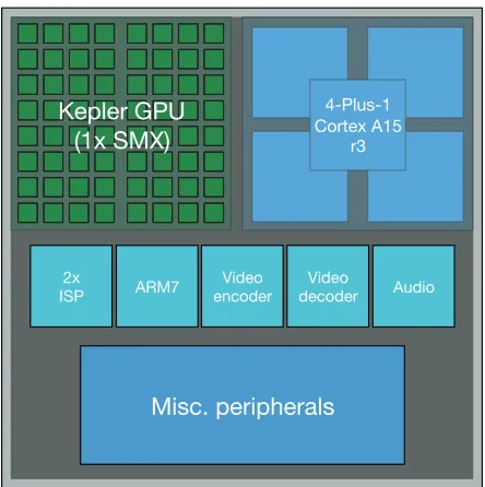
The main processing engine of the Jetson TK1 is the Tegra K1 SoC, which consists of a 4-plus-1 quad-core ARM Cortex A15 CPU and a single Kepler GPU multiprocessor (SMX) with 192 CUDA cores. A schematic of the Tegra K1 SoC is shown in figure 1. Each core can deliver 1 single-precision fused multiply-add (FMA) instruction per cycle. For the rest of this paper, we use only the GPU part of the SoC. The processor will be assumed to be idle and dissipate no energy during an application’s execution other than leakage, as part of the system’s constant power,π0. One downside of this system is that unlike its HPC counterpart, the Tesla GPU series, the double-precision performance is severely limited, with a peak throughput of just1/24×that of single-precision.
The system runs Linux for Tegra (L4T), a modified Ubuntu 14.04 Linux distribution using Linux kernel version 3.10, and at the time of this study included the CUDA 6.0 Toolkit.
PowerMon 2 is a fine-grained integrated power measure-ment device [7]. It sits between the power source and Jetson TK1 and measures the direct current and voltage at a rate of up to 1024 Hz. Figure 2 shows how PowerMon 2 can be connected to our development board and other devices to intercept and measure their current and voltage.
C. Model instantiation
To determine the various constants of the model (Sec-tion II-A), we apply a method similar to what was described in our original energy roofline work [2], [3]. As before, we use our highly-tuned “intensity” microbenchmarks to measure the system’s performance and power consumption.2 However, on top of varying the arithmetic intensity (by changing the number flops executed per word of data loaded from the memory), we also change the frequency and voltage of the processing cores 1Changing the frequency automatically changes the voltage to a pre-determined value.
Kepler GPU
(1x SMX)
4-Plus-1 Cortex A15
r3
2x
ISP ARM7
Video encoder
Video
decoder Audio
Misc. peripherals
Fig. 1: A schematic of the NVIDIA Tegra K1 mobile SoC
ATX PSU
PowerMon 2
PCIe Interposer
GPU
CPU
Motherboard
Input
Output
1 2
1
2
3 4 5 3 4
5 Power Brick
Power Brick
6 7
6 7
ARM Dev Board APU
Fig. 2: Power measurement setup
and the memory system. Out of the 105 possible permutations (15 for the processor and 7 for the memory), we chose 16 settings at random for a total of 1856 sample measurements.
Once we have collected all our performance and power measurements, we apply a non-negative least squares (NNLS) fitting procedure on equation 9 to estimate the constants ˆ
c0,proc,cˆ0,mem,c1,proc, c1,mem, andPmisc. These values are
then used to estimateflop,mem, andπ0using equations 6, 7, and 8. The complete list of frequency and voltage settings, as well as their associated energy and power costs, are shown in table I. One important point to note is that while our model in equation 9 only accounts forW andQto simplify the explana-tion, our actual evaluation differentiates single-precision (SP) and double-precision (DP) flops, and also includes the energy cost of integer operations and loading data from different levels of the memory hierarchy (shared memory, or SM, and L2).
D. Validation
We first validated our model using 2-fold cross validation, also known as the “holdout method” [8]. Measurements from settings of type “T” in table I were used for training the model and deriving the constants, and measurements from setting type “V” were used for validation. When compared to measured energy, the mean error for the validation set was 2.87% with a standard deviation of 2.47%, and the minimum and maximum error were 0.00% and 11.94%, respectively.
We then used 16-fold cross validation to assess how well the model will generalize to an independent data set when used to make predictions for other kernels and applications. The results showed a mean error of 6.56% with a standard deviation of 3.80%, while the minimum and maximum error were 1.60% and 15.22%, respectively.
Our dataset and analysis code, written in R,3 is publicly available for download.4
E. Autotuning for energy
In the context of autotuning for energy, we compare using our model to a method based purely on execution time to find the (fproc,fmem) pair that minimizes energy consumption for a given arithmetic intensity. We assume that we have a “time oracle” that can tell us which configuration yields the best performance. If the idea of “race-to-halt” is true,5 then the configuration that minimizes execution time should do just as well or better than our model in minimizing energy. Table II summarizes our findings.
Our results show that choosing a configuration that yields the best performance (i.e., the smallest execution time) does not always result in the most energy efficient configuration. For example, in the case of the single–precision microbenchmark, adopting the “race–to–halt” strategy resulted in getting an energyinefficientconfiguration20out of25cases (i.e., arith-metic intensity values), whereas our model made the correct prediction every time.
While the energy “lost” by either strategy is relatively small for most benchmarks (under 11% in all but one case), our results show that energy can be saved by changing the frequency and voltage settings even when the computation is uniform. This finding stands in contrast to many other DVFS strategies, which can save energy only in the presence of application “slack.” In section IV we investigate whether this idea can be applied to save energy in a proxy application, which implements the fast multipole method.
III. THE FAST MULTIPOLE METHOD
This section summarizes the fast multipole method, which is the basis for the proxy application we wrote and evaluated in section IV. This summary borrows from some of our earlier papers [5], [9].
3https://www.r-project.org/
4https://bitbucket.org/jee/jetson-tk1-data
5The race-to-halt strategy says that the best way to save energy is to run
Core Core Memory Memory Energy Energy Energy Energy Energy Energy Const.
freq. volt. freq. volt. SP DP Integer SM L2 Mem power
Type (MHz) (mV) (MHz) (mV) (pJ) (pJ) (pJ) (pJ) (pJ) (pJ) (W)
T 852 1030 924 1010 29.0 139.1 60.0 35.4 90.2 377.0 6.8
T 396 770 924 1010 16.2 77.7 33.5 19.8 50.4 377.0 6.1
T 852 1030 528 880 29.0 139.1 60.0 35.4 90.2 286.2 6.3
T 648 890 528 880 21.7 103.8 44.8 26.4 67.3 286.2 5.9
T 396 770 528 880 16.2 77.7 33.5 19.8 50.4 286.2 5.6
T 852 1030 204 800 29.0 139.1 60.0 35.4 90.2 236.5 6.0
T 648 890 204 800 21.7 103.8 44.8 26.4 67.3 236.5 5.6
T 396 770 204 800 16.2 77.7 33.5 19.8 50.4 236.5 5.2
V 756 950 924 1010 24.7 118.3 51.0 30.1 76.7 377.0 6.6
V 180 760 528 880 15.8 75.7 32.7 19.3 49.1 286.2 5.5
V 540 840 528 880 19.3 92.5 39.9 23.5 59.9 286.2 5.8
V 540 840 204 800 19.3 92.5 39.9 23.5 59.9 236.5 5.4
V 756 950 204 800 24.7 118.3 51.0 30.1 76.7 236.5 5.8
V 72 760 68 800 15.8 75.7 32.7 19.3 49.1 236.5 5.2
V 756 950 68 800 24.7 118.3 51.0 30.1 76.7 236.5 5.8
V 180 760 924 1010 15.8 75.7 32.7 19.3 49.1 377.0 6.0
TABLE I: List of frequency and voltage settings, and derived energy and power costs.
Energy lost (%) Mispredictions Mean Minimum Maximum
Single Our model 0 (out of 25) 0 0 0
Time Oracle 20 (out of 25) 18.52 7.21 26.52
Double Our model 10 (out of 36) 3.11 0.34 7.30 Time Oracle 23 (out of 36) 3.95 0.23 13.90
Integer Our model 6 (out of 23) 2.37 0.32 5.12 Time Oracle 23 (out of 23) 3.56 0.44 9.72 Shared Our model 7 (out of 10) 3.31 2.92 3.99 memory Time Oracle 10 (out of 10) 10.64 7.07 12.75
L2 Our model 0 (out of 9) 0 0 0
Time Oracle 0 (out of 9) 10.71 10.49 11.28
TABLE II: Summary of energy autotuning result. “Energy lost” shows how much more energy the incor-rect configuration (mispredictions) chosen by our model and the time oracle dissipated when com-pared to experimentally measured minimum for different microbenchmarks and their intensities.
Given a system ofN sourceparticles, with positions given by{y1, . . . , yN}, andN targetswith positions{x1, . . . , xN}, we wish to compute theN sums,
f(xi) = N
j=1
K(xi, yi)·s(yj), i= 1, . . . , N (10)
wheref(x)is the desiredpotentialat target pointx;s(y)is the
densityat source pointy; andK(x, y)is aninteraction kernel
that specifies “the physics” of the problem. For instance, the single-layer Laplace kernel,K(x, y) = 41π||x−1y||, might model electrostatic or gravitational interactions.
Evaluating these sums appears to require ON2
opera-tions. The FMM instead computes approximations of all of these sums in optimal O(N) time with a guaranteed user-specified accuracy, where the desired accuracy changes the complexity constant [10].
In our previous work, we modeled and implemented [5], [9] thekernel-independent variant of FMM, or KIFMM [11], which has the same structure as the classical FMM [10]. Its main advantage over the classical FMM is that it avoids the mathematically challenging analytic expansion of the kernel, instead requiring only the ability to evaluate the kernel. This feature of the KIFMM allows us to leverage our optimization techniques and apply them to new kernels and problems. For
our evaluation in section IV, we only use the GPU version of FMM.
The FMM is based on two key ideas:
• organizing the points in aspatial tree; and
• usingfast approximate evaluations, in which we com-pute summaries at each node using a constant number of tree traversals with constant work per node.
A. Tree construction
Given the input points and a user-defined parameterQ, we construct an octreeT (or quad-tree in 2D) by starting with a single box representing all the points and recursively subdi-viding each box if it contains more than Qpoints. Each box (octant in 3D or quadrant in 2D) becomes a tree node whose children are its immediate sub boxes. During construction, we associate with each node one or more neighborlists. Each list has bounded constant length and contains (logical) pointers to a subset of other tree nodes. These are canonically known as theU,V,W, andX lists. For example, every leaf boxBhas a U list,U(B), which is the list of all leaves adjacent toB. Figure 3 shows a quad-tree example, where neighborhood list nodes forB are labeled accordingly.
B
X
X
V
V
V V V V
V V
V V
V V
V V
V V
W W W W W U
U
U U
U
U U
B. Evaluation
Given the tree T, evaluating the sums consist of six distinct computation phases; there is one phase for each of theU,V,
W, andXlists, as well asupward(UP) anddownward(DOWN) phases. These phases involve the traversals of T or subsets of T. For a more detailed description of FMM, we refer the readers to [11].
The most important property of FMM in the context of this work is the variability of its arithmetic intensity across different phases. The two most expensive phases of FMM are theUlist andV list computations;Ulist computation is highly compute bound (high arithmetic intensity) as it calculates
OQ2 interactions with the nearest neighbors directly; the V list, on the other hand, is highly memory bandwidth bound (low arithmetic intensity) as it approximates interactions with far neighbors through fast Fourier transforms (FFT) and vector additions. By changing the input parameter Q, we can also change the balance of workload between these two phases so that the FMM’s overall arithmetic intensity can be tailored to a particular platform to maximize performance.
IV. EXPERIMENTAL RESULT AND ANALYSIS OFFMM
We used our model on our FMM implementation to see where energy is being consumed and whether we can leverage the autotuning aspect of our model (section II-E) to choose optimal processor and memory frequency settings on the NVIDIA Jetson TK1. We start by evaluating the accuracy of our model for the FMM kernel by comparing the model’s predicted energy consumption against real measurements for a number of different system settings and kernel parameters (i.e., the total number of pointsN and the maximum number of points per box,Q).
A. Basic profile of the FMM
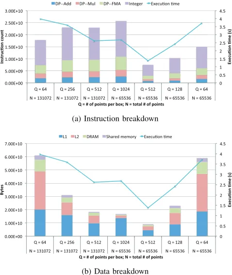
We used thenvprofperformance counter monitor (PCM) to measure instruction counts by type for our FMM imple-mentation. A summary of these counters appears in table III. The counter type “E” is a counter event, which corresponds to a single hardware counter value; and counter type “M” is a counter metric, which is a characteristic of the running application and is derived from one or more counter events.
For the number of instructions, we used the readings given by the corresponding counter event directly. For calculating the number of bytes coming from different levels of the memory hierarchy, we either use a counter metric directly, or infer it by using a combination of different counter metrics and/or events (e.g., reads from the L2 cache can be calculated by subtracting the number of bytes read from the DRAM from the total number ofrequeststo the L2). The breakdown of instructions and data loaded from different levels of the memory hierarchy are shown in figure 4.
Using the instruction and data breakdown of the FMM kernel, and the estimated energy cost of different operations and data access under different frequency settings, we can now predict the total energy consumed by the FMM kernel using equation 9. Since we did not have separate microbenchmarks for add and multiply operations, we use our estimates for the FMA instructions instead. We believe that this is a good estimate, as they all share the same functional units.
# # # ! !# " "#
( #(' ( #( ( #( !(
)$" ) #$ )# ) " )# ) & )$" )!% )!% )!% )$##!$ )$##!$ )$##!$ )$##!$
(a) Instruction breakdown
"
"
" "
!
!"
&
&
& &
!&
"&
#&
$&
'#! '"# '" '! '" '% '#!
' $ ' $ ' $ '#"" # '#"" # '#"" # '#"" #
(b) Data breakdown
Fig. 4: Breakdown of the FMM kernel to component instruc-tions and data access to different levels of the memory hierarchy
B. Validation
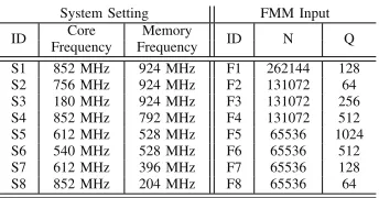
We validate our predictions against real measurements using eight different frequency settings and eight different set of input parameters to the FMM kernel, for a total of 64 test cases. These frequency settings and input parameters to the kernel are summarized in table IV. Figure 5 shows a summary of our evaluation results. The label on the x-axis (e.g., “F1” and “S1”) are IDs that indicate the frequency setting and the input parameters used for that particular test case. (These IDs can be found in table IV.)
Over all 64 test cases, we observed a mean error of 6.17%, with a standard deviation of 4.65%. The error rates also range from as low as 0.09% to as high as 14.89%. These numbers closely match the error rates for the 16–fold cross validation of our microbenchmarks (section II-D).
C. Observations
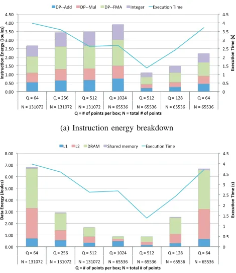
Figure 6 shows the breakdown of energy by type for in-structions and data access for different FMM input parameters when both the processing cores and the memory are running at maximum frequency (852 MHz for the cores, 924 MHz for the memory).
a) Integer instructions overhead: When we study
Type Name Description
M flops dp fma # of double–precision floating point multiply–accumulate operations M flops dp add # of double–precision floating point add operations
M flops dp mul # of double–precision floating point multiply operations M inst integer # of integer instructions
E l1 global load hit # of cache lines that hit in L1 cache E l2 subp0 total read sector queries Total read request for slice 0 of L2 cache E gld request # of load instructions
E l1 shared load transactions # of shared load transactions
E fb subp0 read sectors # of DRAM read request to sub partition 0 E fb subp1 read sectors # of DRAM read request to sub partition 1
E l2 subp0 read l1 hit sectors # of read requests from L1 that hit in slice 0 of L2 cache E l2 subp1 read l1 hit sectors # of read requests from L1 that hit in slice 1 of L2 cache E l2 subp2 read l1 hit sectors # of read requests from L1 that hit in slice 2 of L2 cache E l2 subp3 read l1 hit sectors # of read requests from L1 that hit in slice 3 of L2 cache E gst request # of store instructions
E l2 subp0 total write sector queries Total write request to slice 0 of L2 cache E l1 shared store transactions # of shared store transactions
TABLE III: Summary of counter events and metrics used to create a new of the FMM kernel. Type “E” are events and type “M” are metrics.
$ $ $ $ !$ $ $ $ $
!
! ! ! ! ! ! ! ! !!!!!!!!
$
To
t
a
l Ener
gy (Joules)
Fig. 5: Comparison of estimate vs. measured energy for various test cases
System Setting FMM Input
ID Core Memory ID N Q
Frequency Frequency
S1 852 MHz 924 MHz F1 262144 128 S2 756 MHz 924 MHz F2 131072 64 S3 180 MHz 924 MHz F3 131072 256 S4 852 MHz 792 MHz F4 131072 512 S5 612 MHz 528 MHz F5 65536 1024 S6 540 MHz 528 MHz F6 65536 512 S7 612 MHz 396 MHz F7 65536 128 S8 852 MHz 204 MHz F8 65536 64
TABLE IV: Summary of DVFS settings and input parameters used for validation
for all input parameters (instruction count and data access pattern is mostly independent of system setting). This is not
surprising, as most real applications on modern architectures require large number of loops and address calculations. In contrast, the energy dissipation from integer instructions ac-counts for only about 23% of total energy consumed by computation instructions, regardless of the core’s frequency
setting. This observation suggests that while most applications
“waste” many processing cycles onnot usefulandunavoidable
overhead of integer operations, it does not significantly impact performance or energy consumption. Such a low impact is expected, since integer operations are typically less complex and use different resources in the pipeline from floating point operations.
b) Data access: Although GPUs typically have very
%
!
!%
"
"%
#
#%
$
$%
%
!
!%
"
"%
#
#%
$
$%
)&$ )"%& )%!" )! "$ )%!" )!"( )&$ )!#! '" )!#! '" )!#! '" )&%%#& )&%%#& )&%%#& )&%%#&
! !
(a) Instruction energy breakdown
$ $ ! !$ " "$ # #$
! " # $ % & '
(%# (!$% ($ ! ( !# ($ ! ( !' (%# ( " &! ( " &! ( " &! (%$$"% (%$$"% (%$$"% (%$$"%
! !
!
(b) Data energy breakdown
Fig. 6: Breakdown of the FMM kernel by energy
accesses. However, these accesses still account for up to 50% of the total data access energy. After DRAM, L2 cache accesses account for 30–40% of total data access energy; and for L1 cache accesses, 10-20%. Thus, keeping data close to the core as possible has a large benefit both in terms of performance and energy-efficiency, and can lead to cutting data access energy cost by as much as half.
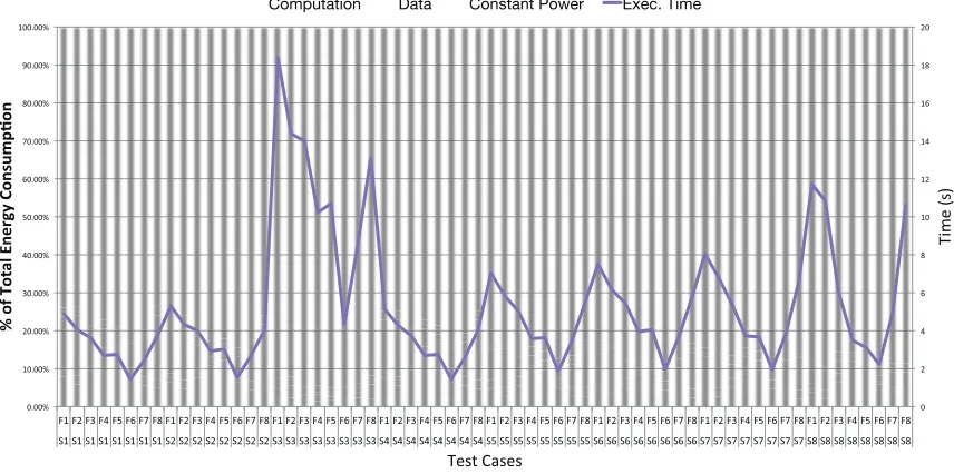
c) Constant power: Figure 7 shows a breakdown of
the total energy dissipation from figure 5. Total energy is broken down to three parts: “Computation” is the total energy consumed by integer, add, multiply, and FMA instructions; “Data” is the total energy consumed by all data access types (SM, L1, L2, and DRAM); ”Constant power” is the energy consumed by constant power over the application’s execution time. The figure also shows the energy consumed by each type as percentage of the total energy rather than in Joules.
The largest contributor to energy consumption is constant power, accounting for anywhere from 75% to 95% of the total energy consumed by the application. For this reason, our model predicts that the best setting for energy efficiency for our FMM kernel is also the setting that yields the best performance. This observation goes against some of the predictions of section II-E.
We believe the problem may be underutilization of hard-ware resources. A similar breakdown of the energy consumed by our microbenchmarks shows that constant power only accounts for about 30% of the total energy. While the
mi-crobenchmarks utilize close to 100% of the targeted resource, this is not the case for our FMM kernel. Compared to the maximum instructions per cycle (IPC) that the system can deliver, our code delivers less than a quarter of that. At first glance, this fact suggests that the kernel is not well-optimized. However, we analyzed theachievable peak given themix of
instructions for the U list phase in our previous work [9].
Assuming there is enough parallelism in our code to hide instruction latency, the best that theU list kernel can achieve is slightly above14of the peak performance of the system, i.e., not all computation in the FMM translate to FMA instructions. Thus, our implementation does not appear to be far from
the achievable peak. More importantly, it also suggests that
many applications are unlikely to come close to delivering a system’s peak performance, and therefore, will also waste a large amount of energy on constant power as they wait for the necessary data or dependencies to be resolved.
V. RELATEDWORK
Frequency scaling and concurrency throttling:
Tech-niques based on DVFS have proven to be effective in mini-mizing energy consumption with little or no impact on per-formance [12]–[17]. DVFS scales down the frequency (and therefore the voltage) when processor speed does not limit performance, taking advantage of the superlinear scaling of power and energy with frequency. Among these, the work by Lively et. al uses principal component analysis (PCA) method to model execution time and power consumption using a small set of performance counters, which is then used to determine the appropriate DVFS and dynamic concurrency throttling (DCT) settings. DCT is a similar technique [18]– [20], where the number of threads or cores (concurrency) is limited to reduce energy consumption when employing an additional core brings limited performance improvement but a large power cost. These approaches, however, are system-centric and not cognizant about algorithmic properties, such as arithmetic intensity, and therefore, they provide no insight to algorithm designers and programmers into what they can do to make programs more energy efficient on their respective systems.
Modeling time, energy, and power: Other modeling
Computation Data Constant Power Exec. Time
Fig. 7: Breakdown of energy consumption by three types: energy spent on computation (incl. integer operations), data movement (from all levels of the memory hierarchy), and constant power (or overhead)
and energy [15], [16], [38]–[41], and like the time-based models, much of this work is system- or architecture-centric, abstracting away algorithmic properties.
Finally, there are a number of microarchitecture simulators that model power dissipation [42]–[44] at the transistor level. Although in theory theymay provide the most accurate esti-mates of power dissipation, they have a number of limitations that prevents from being used in our work. Firstly, simula-tors typically make assumptions about the hardware they are simulating, as no vendor provides a complete transistor-level schematic of their hardware. Secondly, they do not validate their results against real systems rigorously enough; sometimes they only compare their results against the thermal design power (TDP). Lastly, they do not provide any convenient means of interfacing with real software or algorithms.
Computing on embedded system-on-chip: Interest in
embedded/mobile SoC for HPC has grown rapidly in recent years. The most notable and perhaps the largest work is the Mont Blanc project [45] which attempts to build a supercom-puter from low-power, low-performance ARM SoCs. However, they have yet to show definitive results that indicate whether ARM SoCs are the answer to a more energy efficient design. Other work in employing mobile SoC for HPC include [46]– [54], as well as those that use SoC for high-performance general purpose processing such as computer vision and speech processing [55]–[57]; these papers tend to focus onpresenting
the performance and energy dissipation results rather than indicating ways ofimprovingthem, as we do.
VI. CONCLUSION
In this paper, we presented a new method for deriving the energy cost of different operations – such as flops and moving data – for different frequency and voltage settings.
We demonstrated how these values, along with readings from performance counters, can accurately predict the energy con-sumption of not only microbenchmarks, but also a proxy application that is based on the fast multipole method.
We also show that for certain types of applications – those that are simple and highly regular, like our microbenchmarks – run more energy efficiently at certain frequencies, and those settings may not necessarily deliver the best performance, and that our model can accurately predict (autotune) those settings. For the FMM, energy is minimized by the same frequency set-tings that minimize time, due primarily to the large percentage of total energy being consumed by constant power. We hypoth-esize that this effect is caused by system underutilization due to the application’s natural mix of instructions being incapable of achieving a system’s peak performance. Overcoming such underutilization would likely require some combination of aggressive algorithmic rearrangement and microarchitectural improvements (section IV-C).
More so than the results, we wish to emphasize the
method-ological aspect of this research. Users can easily replicate
ACKNOWLEDGMENTS
This work was supported in part by a grant from the US National Science Foundation (NSF) under Award #1422935. Any opinions, findings and conclusions or recommendations expressed in this material are those of the authors and do not necessarily reflect those of NSF.
REFERENCES
[1] A. Snavely, L. Carrington, N. Wolter, J. Labarta, R. Badia, and A. Purkayastha, “A framework for performance modeling and prediction,” in Proceedings of the 2002 ACM/IEEE Conference on Supercomputing (SC), 2002, pp. 1–17. [Online]. Available: http://dl.acm.org/citation.cfm?id=762785
[2] J. Choi, R. Vuduc, R. Fowler, and D. Bendard, “A roofline model of energy,” inIn Proceedings of the 27th IEEE International Parallel and Distributed Processing Symposium (IPDPS 13), 2013.
[3] J. Choi, M. Dukhan, X. Liu, and R. Vuduc, “Algorithmic time, energy, and power on candidate hpc compute building blocks,” inIn Proceed-ings of the 28th IEEE International Parallel and Distributed Processing Symposium (IPDPS 14), 2014.
[4] L. Ying, G. Biros, D. Zorin, and H. Langston, “A new parallel kernel-independent fast multipole method,” inProc. ACM/IEEE Conf. Supercomputing (SC), Phoenix, AZ, USA, November 2003. [Online]. Available: http://portal.acm.org/citation.cfm?id=1050165
[5] A. Chandramowlishwaran, J. W. Choi, K. Madduri, and R. Vuduc, “Towards a communication optimal fast multipole method and its implications for exascale,” inProc. ACM Symp. Parallel Algorithms and Architectures (SPAA), Pittsburgh, PA, USA, June 2012, brief announcement.
[6] S. Kaxiras and M. Martonosi, Computer Architecture Techniques for Power-Efficiency, 1st ed. Morgan and Claypool Publishers, 2008. [7] D. Bedard, M. Y. Lim, R. Fowler, and A. Porterfield, “Powermon:
Fine-grained and integrated power monitoring for commodity computer systems,” inIEEE SoutheastCon 2010 (SoutheastCon), Proceedings of the, march 2010, pp. 479 –484.
[8] S. Geisser,Predictive inference. CRC Press, 1993, vol. 55. [9] J. Choi, A. Chandramowlishwaran, K. Madduri, and R. Vuduc,
“A cpu: Gpu hybrid implementation and model-driven scheduling of the fast multipole method,” in Proceedings of Workshop on General Purpose Processing Using GPUs, ser. GPGPU-7. New York, NY, USA: ACM, 2014, pp. 64:64–64:71. [Online]. Available: http://doi.acm.org/10.1145/2576779.2576787
[10] L. Greengard and V. Rokhlin, “A fast algorithm for particle simulations,”
J. Comp. Phys., vol. 73, pp. 325–348, 1987.
[11] L. Ying, D. Zorin, and G. Biros, “A kernel-independent adaptive fast multipole method in two and three dimensions,”J. Comp. Phys., vol. 196, pp. 591–626, May 2004.
[12] R. Ge, X. Feng, and K. W. Cameron, “Performance-constrained distributed dvs scheduling for scientific applications on power-aware clusters,” in Proceedings of the 2005 ACM/IEEE conference on Supercomputing, ser. SC ’05. Washington, DC, USA: IEEE Computer Society, 2005, pp. 34–. [Online]. Available: http://dx.doi.org/10.1109/SC.2005.57
[13] V. W. Freeh, D. K. Lowenthal, F. Pan, N. Kappiah, R. Springer, B. L. Rountree, and M. E. Femal, “Analyzing the energy-time trade-off in high-performance computing applications,” IEEE Trans. Parallel Distrib. Syst., vol. 18, no. 6, pp. 835–848, Jun. 2007. [Online]. Available: http://dx.doi.org/10.1109/TPDS.2007.1026
[14] Y. Jiao, H. Lin, P. Balaji, and W. Feng, “Power and performance char-acterization of computational kernels on the gpu,” inGreen Computing and Communications (GreenCom), 2010 IEEE/ACM Int’l Conference on Int’l Conference on Cyber, Physical and Social Computing (CP-SCom), dec. 2010, pp. 221 –228.
[15] R. Ge and K. Cameron, “Power-aware speedup,” inIn Proceedings of the 21st IEEE International Parallel and Distributed Processing Symposium (IPDPS 07), 2007.
[16] S. Song, M. Grove, and K. W. Cameron, “An iso-energy-efficient approach to scalable system power-performance optimization,” in Proceedings of the 2011 IEEE International Conference on Cluster Computing, ser. CLUSTER ’11. Washington, DC, USA: IEEE Computer Society, 2011, pp. 262–271. [Online]. Available: http://dx.doi.org/10.1109/CLUSTER.2011.37
[17] C. Lively, V. Taylor, X. Wu, H.-C. Chang, C.-Y. Su, K. Cameron, S. Moore, and D. Terpstra, “E-amom: an energy-aware modeling and optimization methodology for scientific applications,” Computer Science - Research and Development, vol. 29, no. 3-4, pp. 197–210, 2014. [Online]. Available: http://dx.doi.org/10.1007/s00450-013-0239-3 [18] M. Curtis-Maury, J. Dzierwa, C. D. Antonopoulos, and D. S. Nikolopoulos, “Online power-performance adaptation of multithreaded programs using hardware event-based prediction,” inProceedings of the 20th Annual International Conference on Supercomputing, ser. ICS ’06. New York, NY, USA: ACM, 2006, pp. 157–166. [Online]. Available: http://doi.acm.org.prx.library.gatech.edu/10.1145/1183401.1183426 [19] K. Chakraborty, “A case for an over-provisioned multicore system:
Energy efficient processing of multithreaded programs,” University of Wisconsin Madison, Tech. Rep., 2007.
[20] M. Curtis-Maury, A. Shah, F. Blagojevic, D. S. Nikolopoulos, B. R. de Supinski, and M. Schulz, “Prediction models for multi-dimensional power-performance optimization on many cores,” in Proceedings of the 17th International Conference on Parallel Architectures and Compilation Techniques, ser. PACT ’08. New York, NY, USA: ACM, 2008, pp. 250–259. [Online]. Available: http://doi.acm.org.prx.library.gatech.edu/10.1145/1454115.1454151 [21] K. Czechowski, C. Battaglino, C. Mcclanahan, A.
Chandramowlish-waran, and R. Vuduc, “Balance principles for algorithm-architecture co-design,” inUSENIX Wkshp. Hot Topics in Parallelism (HotPar). Berke-ley, CA, USA: Usenix Association, 2011, pp. 1–5. [Online]. Available: http://www.usenix.org/event/hotpar11/tech/final files/Czechowski.pdf [22] K. Czechowski and R. Vuduc, “A theoretical framework for
algorithm-architecture co-design,” in Parallel Distributed Processing (IPDPS), 2013 IEEE 27th International Symposium on, 2013, pp. 791–802. [23] M. D. Hill and M. R. Marty, “Amdahl’s Law in the Multicore
Era,”Computer, vol. 41, no. 7, pp. 33–38, Jul. 2008. [Online]. Available: http://ieeexplore.ieee.org/lpdocs/epic03/wrapper.htm?arnumber=4563876 [24] D. H. Woo and H.-H. S. Lee, “Extending Amdahl’s Law for
energy-efficient computing in the many-core era,”IEEE Computer, vol. 41, no. 12, pp. 24–31, Dec. 2008.
[25] T. Zidenberg, I. Keslassy, and U. Weiser, “Multi-Amdahl: How Should I Divide My Heterogeneous Chip?” IEEE Computer Architecture Letters, pp. 1–4, 2012. [Online]. Available: http://ieeexplore.ieee.org/lpdocs/epic03/wrapper.htm?arnumber=6175876 [26] H. T. Kung, “Memory requirements for balanced computer
architec-tures,” inProceedings of the ACM Int’l. Symp. Computer Architecture (ISCA), Tokyo, Japan, 1986.
[27] W. D. Hillis, “Balancing a Design,”IEEE Spectrum, 1987. [Online]. Available: http://longnow.org/essays/balancing-design/
[28] R. W. Hockney and I. J. Curington, “f1/2: A parameter to characterize memory and communication bottlenecks,” Parallel Computing, vol. 10, no. 3, pp. 277–286, May 1989. [Online]. Available: http://linkinghub.elsevier.com/retrieve/pii/0167819189901002 [29] G. E. Blelloch, B. M. Maggs, and G. L. Miller, “The hidden cost of
low bandwidth communication,” inDeveloping a Computer Science Agenda for High-Performance Computing, U. Vishkin, Ed. New York, NY, USA: ACM, 1994, pp. 22–25.
[30] J. McCalpin, “Memory Bandwidth and Machine Balance in High Performance Computers,” IEEE Technical Committee on Computer Architecture (TCCA) Newsletter, Dec. 1995. [Online]. Available: http://www.cs.virginia.edu/ mccalpin/papers/balance/index.html [31] S. Williams, A. Waterman, and D. Patterson, “Roofline: an insightful
visual performance model for multicore architectures,” Commun. ACM, vol. 52, no. 4, pp. 65–76, Apr. 2009. [Online]. Available: http://doi.acm.org/10.1145/1498765.1498785
[33] S. Keckler, W. Dally, B. Khailany, M. Garland, and D. Glasco, “Gpus and the future of parallel computing,”Micro, IEEE, vol. 31, no. 5, pp. 7 –17, sept.-oct. 2011.
[34] C. M. Olschanowsky, T. Rosing, A. Snavely, L. Carrington, M. M. Tikir, and M. Laurenzano, “Fine-grained energy consumption characterization and modeling,” in High Performance Computing Modernization Pro-gram Users Group Conference (HPCMP-UGC), 2010 DoD, June 2010, pp. 487–497.
[35] S. Hong and H. Kim, “An analytical model for a GPU architecture with memory-level and thread-level parallelism awareness,” inProceedings of the 36th annual International Symposium on Computer Architecture (ISCA). New York, NY, USA: ACM, 2009, pp. 152–163. [Online]. Available: http://doi.acm.org/10.1145/1555754.1555775
[36] S. S. Baghsorkhi, M. Delahaye, S. J. Patel, W. D. Gropp, and W. mei W. Hwu, “An adaptive performance modeling tool for GPU architectures,”SIGPLAN Not., vol. 45, no. 5, pp. 105–114, Jan. 2010. [Online]. Available: http://doi.acm.org/10.1145/1837853.1693470 [37] Y. Zhang and J. D. Owens, “A quantitative performance
analysis model for gpu architectures,” in Proceedings of the 2011 IEEE 17th International Symposium on High Performance Computer Architecture, ser. HPCA ’11. Washington, DC, USA: IEEE Computer Society, 2011, pp. 382–393. [Online]. Available: http://dl.acm.org/citation.cfm?id=2014698.2014875
[38] C. Lively, X. Wu, V. Taylor, S. Moore, H.-C. Chang, C.-Y. Su, and K. Cameron, “Power-aware predictive models of hybrid (MPI/OpenMP) scientific applications on multicore systems,” Computer Science -Research and Development, pp. 1–9, 2011, 10.1007/s00450-011-0190-0. [Online]. Available: http://dx.doi.org/110.1007/s00450-011-0190-0.1007/s00450-011-0190-0 [39] B. Subramaniam and W.-C. Feng, “Statistical power and performance
modeling for optimizing the energy efficiency of scientific computing,” in Proceedings of the 2010 IEEE/ACM Int’l Conference on Green Computing and Communications & Int’l Conference on Cyber, Physical and Social Computing, ser. GREENCOM-CPSCOM ’10. Washington, DC, USA: IEEE Computer Society, 2010, pp. 139–146. [Online]. Available: http://dx.doi.org/10.1109/GreenCom-CPSCom.2010.138 [40] S. Hong and H. Kim, “An integrated GPU power
and performance model,” SIGARCH Comput. Archit. News, vol. 38, no. 3, pp. 280–289, Jun. 2010. [Online]. Available: http://doi.acm.org/10.1145/1816038.1815998
[41] C. Su, D. Li, D. Nikolopoulos, K. Cameron, B. de Supinski, and E. Leon, “Model-based, memory-centric performance and power opti-mization on numa multiprocessors,” inIEEE International Symposium on Workload Characterization, Nov. 2012.
[42] S. J. E. Wilton and N. P. Jouppi, “Cacti: An enhanced cache access and cycle time model,”IEEE Journal of Solid-State Circuits, vol. 31, pp. 677–688, 1996.
[43] S. Li, J. H. Ahn, R. D. Strong, J. B. Brockman, D. M. Tullsen, and N. P. Jouppi, “Mcpat: An integrated power, area, and timing modeling framework for multicore and manycore architectures,” in Proceedings of the 42Nd Annual IEEE/ACM International Symposium on Microarchitecture, ser. MICRO 42. New York, NY, USA: ACM, 2009, pp. 469–480. [Online]. Available: http://doi.acm.org/10.1145/1669112.1669172
[44] J. Leng, T. Hetherington, A. ElTantawy, S. Gilani, N. S. Kim, T. M. Aamodt, and V. J. Reddi, “Gpuwattch: Enabling energy optimizations in gpgpus,” in Proceedings of the 40th Annual International Symposium on Computer Architecture, ser. ISCA ’13. New York, NY, USA: ACM, 2013, pp. 487–498. [Online]. Available: http://doi.acm.org/10.1145/2485922.2485964
[45] N. Rajovic, L. Vilanova, C. Villavieja, N. Puzovic, and A. Ramirez, “The low power architecture approach towards exascale computing,” Journal of Computational Science, no. 0, pp. –, 2013. [Online]. Available: http://www.sciencedirect.com/science/article/pii/S1877750313000148 [46] K. F¨urlinger, C. Klausecker, and D. Kranzlm¨uller, “Towards energy
efficient parallel computing on consumer electronic devices,” in
Proceedings of the First international conference on Information and communication on technology for the fight against global warming, ser. ICT-GLOW’11. Berlin, Heidelberg: Springer-Verlag, 2011, pp. 1–9. [Online]. Available: http://dl.acm.org/citation.cfm?id=2035539.2035541 [47] V. Janapa Reddi, B. C. Lee, T. Chilimbi, and K. Vaid, “Web search
using mobile cores: quantifying and mitigating the price of efficiency,”
SIGARCH Comput. Archit. News, vol. 38, no. 3, pp. 314–325, Jun. 2010. [Online]. Available: http://doi.acm.org/10.1145/1816038.1816002 [48] P. Stanley-Marbell and V. Cabezas, “Performance, power, and thermal analysis of low-power processors for scale-out systems,” inParallel and Distributed Processing Workshops and Phd Forum (IPDPSW), 2011 IEEE International Symposium on, 2011, pp. 863–870.
[49] I. Grasso, P. Radojkovic, N. Rajovic, I. Gelado, and A. Ramirez, “Energy efficient hpc on embedded socs: Optimization techniques for mali gpu,” inParallel and Distributed Processing Symposium, 2014 IEEE 28th International, May 2014, pp. 123–132.
[50] A. Maghazeh, U. Bordoloi, P. Eles, and Z. Peng, “General purpose computing on low-power embedded gpus: Has it come of age?” in
Embedded Computer Systems: Architectures, Modeling, and Simulation (SAMOS XIII), 2013 International Conference on, July 2013, pp. 1–10. [51] N. Rajovic, P. M. Carpenter, I. Gelado, N. Puzovic, A. Ramirez, and M. Valero, “Supercomputing with commodity cpus: Are mobile socs ready for hpc?” inProceedings of the International Conference on High Performance Computing, Networking, Storage and Analysis, ser. SC ’13. New York, NY, USA: ACM, 2013, pp. 40:1–40:12. [Online]. Available: http://doi.acm.org/10.1145/2503210.2503281
[52] S. Mu, C. Wang, M. Liu, D. Li, M. Zhu, X. Chen, X. Xie, and Y. Deng, “Evaluating the potential of graphics processors for high performance embedded computing,” in Design, Automation Test in Europe Conference Exhibition (DATE), 2011, March 2011, pp. 1–6. [53] L. Stanisic, B. Videau, J. Cronsioe, A. Degomme, V.
Marangozova-Martin, A. Legrand, and J.-F. Mehaut, “Performance analysis of hpc applications on low-power embedded platforms,” inDesign, Automation Test in Europe Conference Exhibition (DATE), 2013, March 2013, pp. 475–480.
[54] N. Rajovic, A. Rico, J. Vipond, I. Gelado, N. Puzovic, and A. Ramirez, “Experiences with mobile processors for energy efficient hpc,” in
Design, Automation Test in Europe Conference Exhibition (DATE), 2013, March 2013, pp. 464–468.
[55] K. Gupta and J. D. Owens, “Compute & memory optimizations for high-quality speech recognition on low-end gpu processors,” in Proceedings of the 2011 18th International Conference on High Performance Computing, ser. HIPC ’11. Washington, DC, USA: IEEE Computer Society, 2011, pp. 1–10. [Online]. Available: http://dx.doi.org/10.1109/HiPC.2011.6152741
[56] Y.-C. Wang and K.-T. Cheng, “Energy-optimized mapping of applica-tion to smartphone platform; a case study of mobile face recogniapplica-tion,” in
Computer Vision and Pattern Recognition Workshops (CVPRW), 2011 IEEE Computer Society Conference on, June 2011, pp. 84–89. [57] G. Wang, Y. Xiong, J. Yun, and J. Cavallaro, “Accelerating computer