Aquacultural system management tool II: analytical and management
capability
Chinenye Chukwuemeka Anyadike
1*, Constantile Crowner Mbajiorgu
1,
Genesis Nnaemeka Ajah
2(1. Department of Agricultural and Bioresources Engineering, University of Nigeria, Nsukka; Nsukka Road 410001; 2. Department of Electrical Engineering, University of Nigeria, Nsukka)
Abstract: It is difficult to analyze the complex system by using conventional tools such as field experimentation and inventory monitoring. Thus, one of the major objectives is used to develop an ecosystem model as a tool for analysis for complex systems. In view of this, the Aquacultural System Management Tool (AQUASMAT) model, which was developed based on existing ecosystem model theories and coded using the C-sharp language, was used to conduct a modeling study on a static concrete fish tank, to demonstrate its managerial and analytical capabilities. The input variables for model execution were site specific parameters, fish/feed parameters, water quality parameters and management options from selected fish farm in Nigeria. The model simulation was for concrete tanks with surface area of 1 m2 and 50 m2, respectively, running for 151 periods by using various management techniques and varied feeding rates. Series of simulations were used to evaluate the ability of the model predicting the effects of different feed regimes, management intensities, budgetary requirements (solely based on the cost of fish and feed), and interaction of parameters over a range of fish production levels. The model was used to gain insight into the dynamics and interactions of major water quality parameters with respect to feed loading and fish growth in a 1 m3 fish tank. The simulation result was compared to a farmer’s production output, and then the best management practices will be provided to the user (farmer), such as the optimal feeding techniques and practices with lower feed conversation ratio (FCR) within recommended range. The relationships and interaction between water parameters with respect to feed loading and fish growth were used to gain insight in sizing the biofilter for aquaponics systems.
Keywords: AQUASMAT, simulation, analysis, management, capability, water quality, inter-relationships
Citation: Anyadike, C. C., C. C. Mbajiorgu, G. N. Ajah. 2017. Aquacultural system management tool II: analytical and management capability. Agricultural Engineering International: CIGR Journal, 19(3): 97–104.
1 Introduction
The objective of intensive aquaculture practice is to
increase profitability by maximizing harvest weight
(biomass) per unit volume/area of production system.
However, these practices always exceed the biological
carrying capacity of the production unit. As for livestock
production, overcrowding usually leads to problems of
environmental degradation, disease, off-flavor (aquatic
animals), and a reduction in individual performance of
the cultured species (Wurts and Wynne, 1996; Tucker,
Received date: 2017-03-24 Accepted date: 2017-07-20 * Corresponding author: Chinenye Chukwuemeka Anyadike, Department of Agricultural and Bioresources Engineering, University of Nigeria, Nsukka. Tel: +2348038741426, Email: [email protected].
2000). Hence, the success and profitability of aquaculture
production is highly dependent on the proper
management employed during the culture period.
Management in aquaculture is synonymous with water
management as water of suitable quality and quantity is a
pre-requisite for any successful aquaculture production. A
good knowledge and understanding of the fish
environment (water) is a prerequisite for increased
production. Thus, the AQUASMAT model, which
involved in the formulation of theoretical relationships
for intensive tank-based fish culture from existing models,
coded with Microsoft® Visual C# (C-sharp), was
developed (Anyadike et al., 2015). The model was
designed to predict the effect of different management
operations on fish yield, to identify and quantify the cause,
and to suggest remedial actions for impaired systems. It
also predicts economic viability of the production system
based on the cost input used in the system, and tracks the
fate of many water quality parameters which are not
readily measured. The primary objective of this paper is
to demonstrate the managerial and analytical capability of
the AQUASMAT. Another objective is to evaluate the
managerial and analytical capabilities of the
AQUASMAT, which include optimizing fish feed input
in the production system and maximizing production,
predicting the relationships and interactions between
critical water quality parameters in order to improve fish
health and growth rates, and modeling nitrogen
requirement to aid sizing of biofilter (grow bed) in
aquaponics system.
2 Methodology
The model development, general characteristics and
implementation have been described as report by
Anyadike et al. (2015). The design of the model involved
synthesizing selected processes and interactions into a
computational framework to simulate the conditions in a
static concrete fish tank, and to reproduce the desired
system response over a selected culture period. The
system variables were grouped into components and
organized for implementation as subroutines. The
subroutines interacted with each other through the main
program which calls them in appropriate sequence. These
sub-routines are: initialization, site parameters, biota, feed,
water quality, organic matter, economic, report
generation and management. The main program
flowchart for the simulation procedure was reported by
Anyadike et al. (2015).
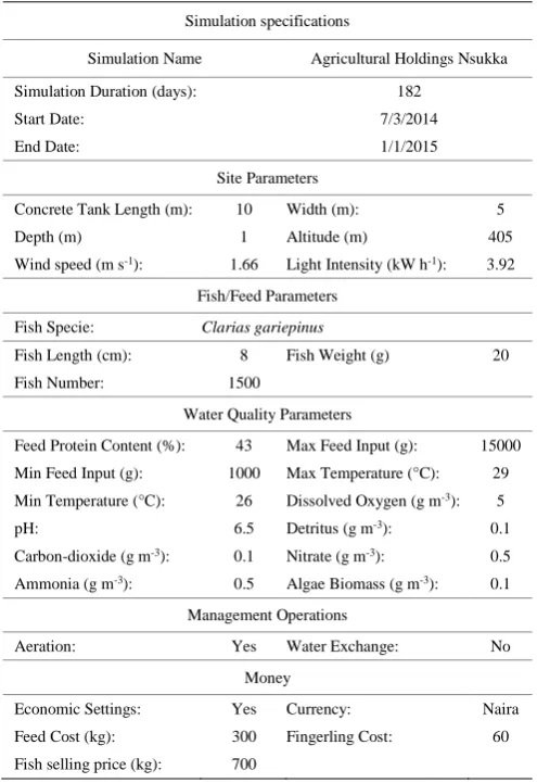
The model is applied in some fish farms in Enugu
State, Nigeria (details of the input specification is
presented in Table 1) at farmer’s minimum and maximum
daily feeding rations of 1000 g (equivalent to feeding rate
of 3.33%) and 15000 g (equivalent to feeding rate of
1.25%) respectively. The result showed that the
maximum biomass was not equal to the maximum profit
as illustrated by Anyadike et al. (2015). The model
suggested remedial action, especially variation of feed at
overfeeding and underfeeding period of production
(Table 2), which was disseminated through seminars,
workshops, and interactions with the farmers. This aid the
choice of a minimum and maximum varied feeding input
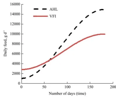
(VFI) of 9% (2800 g daily) and 1% (10000 g),
respectively. The VFI were compared to a real-life
system, Aquaculture Holdings Ltd (AHL) feeding rates, which represent the typical farmer’s management practices in South-Eastern Nigeria. This was done to
ascertain the economic viability and optimum
productivity and efficiency of the production system
based on the cost of input (feed) at 30 fish m-2.
Furthermore, the AQUASMAT model was used to
predict culture conditions in an experimental tank of
1 m×1 m×1 m (water depth of 0.75 m) stocked with 5 g
of Clarias at 14 fish m-2 (Simulation name: clarias14).
The input specifications used to execute the model are
presented in Table 3. This was done to give insight into
the water quality variables and interactions, nitrogen
dynamics and sizing of biofilter for aquaponics systems,
thereby helping stakeholders in evaluating aquaponics
(integrating aquaculture with agriculture) system
adequacy and feasibility.
Table 1 The input specifications used to execute the model
Simulation specifications
Simulation Name Agricultural Holdings Nsukka
Simulation Duration (days): 182
Start Date: 7/3/2014
End Date: 1/1/2015
Site Parameters
Concrete Tank Length (m): 10 Width (m): 5
Depth (m) 1 Altitude (m) 405
Wind speed (m s-1): 1.66 Light Intensity (kW h-1): 3.92
Fish/Feed Parameters
Fish Specie: Clarias gariepinus
Fish Length (cm): 8 Fish Weight (g) 20
Fish Number: 1500
Water Quality Parameters
Feed Protein Content (%): 43 Max Feed Input (g): 15000
Min Feed Input (g): 1000 Max Temperature (°C): 29
Min Temperature (°C): 26 Dissolved Oxygen (g m-3): 5
pH: 6.5 Detritus (g m-3): 0.1
Carbon-dioxide (g m-3): 0.1 Nitrate (g m-3): 0.5
Ammonia (g m-3): 0.5 Algae Biomass (g m-3): 0.1
Management Operations
Aeration: Yes Water Exchange: No
Money
Economic Settings: Yes Currency: Naira
Feed Cost (kg): 300 Fingerling Cost: 60
Table 2 Management regimes suggested by AQUASMAT model for AHL fish farm
Days Parameter Effect Suggested Management
Day 1 to Day 37 FCR FCR from day 1 (0.03351) to day 37 (0.49034): Fish weight gain is poor. Feed fish its percentage body weight
Day 15 to Day 182 Stocking Density Stocking Density from day 15 (2087.46571 g m-2) to day 182 (20155.64826 g m-2). At carrying capacity growth is reduced, feeding is reduced
Reduce fish biomass, increase water exchange, reduce feeding
Day 116 to Day 182 FCR. FCR from day 116 (2.01312) to day 182 (2.4897): High FCR, fish is overfed and at
least 50% of feed is wasted, It can also lead to the introduction of waste in pond Reduce feed to maintenance ration
Table 3 AQUASMAT model simulation input details for African catfish culture in experimental tanks at different stocking densities
Input information Description
Duration Simulation period of 5 months (151 days)
Site Concrete tank of dimension 1 m×1 m×1 m (water depth = 0.75 m)
Altitude was 405 m, wind speed was 1.66 m s-1, light intensity was held constant at 3.91 Kwh m-2 day
Fish and feed data
Number of fish stocked was 14 fish in tank 2, measuring 5 g and 8 cm average weight and length, respectively. Feed was modeled as dynamic with minumum feeding rate of 5% of fish body weight (1.75 g) and maximum daily feed at 1.5% body weight (63 g). Percentage protein content of feed used was 40.4%
Water quality parameters
Temperature and pH were modeled as dynamic between 26°C-29°C and 6.5 respectively. Initial concentration of DO was 4 mg L-1,
CO2 = 0.9, TAN and NO3 = 0.01 mg L-1, Detritus = 0.01 g m-3, and Algae at 0.1 g m-3. Aeration was performed throughout
simulation period.
Economic settings The simulation was performed without the economic option (not available).
The coefficient of determination was used to
statistically assess the goodness-of-fit between observed
and predicted values, and to establish some regression
relationships.
3 Results and Discussion
3.1 Fish growth performance
As shown in Figure 1, the model simulation with farmer’s feeding rate AHL and varied feeding input (VFI) on fish weight gain was at the same facility and stocking
density. However, the cost of achieving the same average
fish weight was observed to be cheaper than the VFI. The
quantity of feed used by AHL was higher than that by
VFI (Figure 2). It showed that a FCR was over than 2
(Figure 3), suggesting that more than half of the feed
introduced to the concrete fish tank by the farmer was
wasted (Isyagi et al., 2009; Timmons and Ebeling, 2010)
daily. In addition, it has been reported that FCR <0.5
suggested underfeeding using the farmer’s feeding rates
(Isyagi et al., 2009). The feeding regime employed by the
farmer (AHL) was therefore found to be flawed as
underfeeding was observed in the first few weeks
(5 weeks) of simulation and feed wastage from the 12th
week. This is in contrast with the modified feeding
regime (VFI), which was within acceptable range throughout the simulation. The effect of the farmer’s high feeding rate was simulated as shown in Figure 4. The
unionized ammonia rate was higher in greater parts of the
simulation for AHL compared to the simulated VFI. Thus,
the most suitable feeding rate as predicted under the two
different scenarios could be used in maximizing
production.
Figure 1 Comparison between the effect of AHL and VFI feeding regime on average weight of African catfish
Figure 3 The comparison of FCR between AHL and VFI
Figure 4 The unionized ammonia (NH3) over a period of time for AHL and VFI
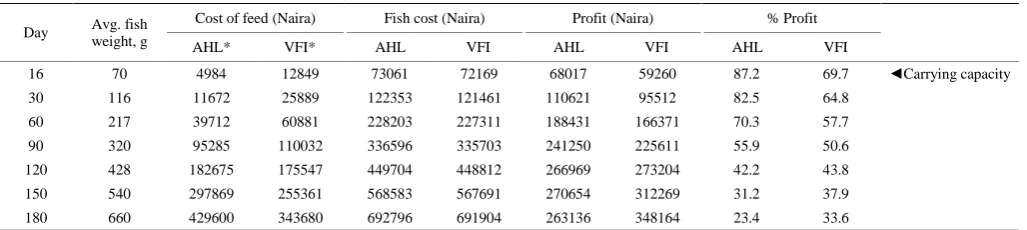
An abridged result generated by AQUASMAT for
AHL and VFI was presented on Table 4. The simulations
attained the carrying capacity that the average weight of
fish was 70 g on day 16. The weight gain at carrying
capacity was observed to be poor, which was in
agreement with the report by Isyagi et al. (2009). The
simulation result of VFI showed more feed input than that
of AHL at the earlier stage (day 1 to day 30). In contrast,
as shown in Figure 3, the FCR was observed to be within
the recommended range of 2 (Isyagi et al., 2009).
Furthermore, the result of AHL recorded more percentage
profit early in the simulation but the margin was observed
to be small as more than 50% of feed was wasted from
the 12th week. This result contributed to the poor water
quality output observed in simulation result of AHL.
Meanwhile, there was a 20% difference in final feed cost
between AHL and VFI as shown in Table 4. The
simulation result also showed that there was 10% extra
profit from VFI than that of AHL, and VFI was at better
water quality. This result was expected since the AHL
regime had incurred losses from wasted feed and poor
fish growth induced by poor water quality. Hence, extra
resources were required in managing the predicted poor
water quality of AHL, despite poor production when
compared with VFI.
Table 4 Cost of production at farmer’s feeding rates (AHL) and simulated varied feeding rates (VFI)
Day Avg. fish weight, g
Cost of feed (Naira) Fish cost (Naira) Profit (Naira) % Profit
AHL* VFI* AHL VFI AHL VFI AHL VFI
16 70 4984 12849 73061 72169 68017 59260 87.2 69.7 ◄Carrying capacity
30 116 11672 25889 122353 121461 110621 95512 82.5 64.8
60 217 39712 60881 228203 227311 188431 166371 70.3 57.7
90 320 95285 110032 336596 335703 241250 225611 55.9 50.6
120 428 182675 175547 449704 448812 266969 273204 42.2 43.8
150 540 297869 255361 568583 567691 270654 312269 31.2 37.9
180 660 429600 343680 692796 691904 263136 348164 23.4 33.6
Note: *AHL is feeding rate at 3.3% initial and 1.25% final; *VF is varied feeding input at 9.33% and 1%.
3.2 Model simulation of African catfish cultured in
experimental tank
The success of a commercial aquaculture enterprise
depends on providing the optimum environment for rapid
growth at the minimum cost of resources and capital. One
of the designed objectives of the AQUASMAT model is
to predict the aquatic environment and critical water
quality parameters so as to optimize fish health and
growth rates. The aquatic environment is a complex
eco-system consisting of multiple water quality variables,
however few critical parameters such as temperature,
suspended solids, and pH and concentrations of dissolved
oxygen, ammonia, nitrite, CO2, and alkalinity, play
decisive roles. Each water quality parameter interacts
with and affects other parameters, sometimes in complex
ways, affects the healthy and growth rate of the fish
(Ebeling, 2015).
In view of this, the model, which predicted the results
of fish stocked at 14 fish m-2, was used to establish and
static tank system with respect to feed loading and fish
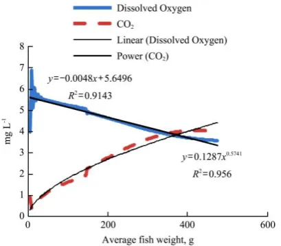
growth. The relationship and interaction of dissolved
oxygen and carbon-dioxide with respect to fish weight is
shown in Figure 5.
Figure 5 Dissolved oxygen and carbon_dioxide (CO2) against weight of fish
The predicted result showed an increase in
carbon-dioxide as dissolved oxygen decreases. The result
of this particular situation showed that there was less
oxygen available to the fish and the fishes were less able
to use the available oxygen. The high carbon dioxide
level of the water affected the fishes' blood capacity to
transport oxygen, aggravating the stress imposed by low
dissolved oxygen levels especially as the average fish
weight increased (Ebeling, 2015). The model was able to
demonstrate that oxygen consumption was a function of
fish body weight, however, respiration per unit biomass
was the greatest for small fish. This result was in
agreement with the observation of Hargreaves and
Tomasso (2004). From the regression analysis, the (R2)
value of body weight on dissolved oxygen consumption
and body weight on carbon-dioxide released by
respiration were 0.914 and 0.956, respectively. However,
the relationship is linear for dissolved oxygen and
average fish weight unlike the relationship between
average fish weight and carbon dioxide released which is
non-linear. Other examples (Figure 6) showed the
relationship between un-ionized ammonia (NH3) and
detritus (organic matter). Despite high rate of organic
matter addition to catfish tank, the accumulation of
sediment organic matter is low and in agreement with
Tucker (1985). However, the absence of dissolved
oxygen to fully mineralize the organic matter caused
temporary accumulation which increased the level of
un-ionized ammonia in the system as suggested by
Hargreaves and Tucker (2003).
Figure 6 Relationship between unionized ammonia and detritus
The relationship between pH and carbon-dioxide
(CO2) is as presented in Figure 7. The pH of water
decreased with the increased CO2, which was in
agreement with Boyd and Tucker (1998). The regression
analysis of the relationship between pH and CO2
indicated an R2 value of 0.9. This showed strong
predictability of the model to forecast accurately. The
relationshipis logarithmic and can be expressed as:
pH=–0.44lnCO2+6.3268 (1)
Figure 7 Relationship between pH and CO2
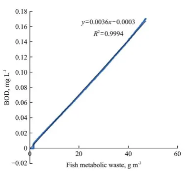
The relationship between rates of oxygen consumption
by bacteria in oxidizing waste generated in the system
Figure 8. The increase of metabolic waste increased
biochemical oxygen demand (Timmons and Ebeling,
2010; Pillay, 2004; Tucker et al., 2008). The regression
analysis established a linear relationship between
metabolic waste generated by fish and oxygen required to
decompose this waste. This was directly proportional to
rate of metabolic waste generated by fish and was
presented in Equation (2).
y=0.0036x–0.003 (2)
Figure 8 Relationship between fish metabolic waste and BOD
The relationships between temperature, dissolved
oxygen and fish respiration were also predicted that
temperature affected virtually all processes in the system
(Park et al., 2009). Figure 9 was a predicted model result
relating to temperature and dissolved oxygen (DO). DO
levels were observed to reduce with increased
temperature (Park and Clough, 2012). Fish metabolic rate
was also observed to be highly influenced by temperature
as presented in Figure 10. The AQUASMAT model
predicted an increase in metabolic rate with a peak
activity at temperature of 27°C before a slow decline
which continued to increases with temperature and
becomes limiting, which was in agreement with the
previous report (Hargreaves and Tomasso, 2004). This
temperature at peak activity was within the range of
optimal temperature required for production of catfish as
suggested by Hecht et al. (1988) and Isyagi et al. (2009).
The predicted model result was in agreement with
Ebeling (2015) that the environmental temperature
changes affected the fishes' rate of biochemical reactions,
leading to different metabolic and oxygen consumption
rates. At the lower ranges of the species tolerable
temperature range, these rates decreased. As water
temperatures increased, fish became more active and
consumed more dissolved oxygen, while simultaneously
produced more carbon dioxide and other excretory
products, such as ammonia. These increasing rates of
consumption of necessary elements and production of
detrimental elements had a direct effect on overall fish
healthy and survival rate if these parameters were allowed
to exceed nominal values. If it was not corrected, the fish
will become stressed to some degree. Even low levels of
stress can have adverse long-term consequences in the
form of reducing growth rates or mortality due to
opportunistic organisms that take advantage of the
stressed fish.
Figure 9 Relationship between temperature and DO
Figure 10 Relationship between temperature and fish metabolic rate
3.3 Modeling nitrogen requirement for sizing biofilter
(grow bed) in aquaponics system
The biofilter, a major component of the aquaculture
treatment unit, was used to remove the total ammonia
nitrogen to a recommended level of 1 ppm through
nitrification (Al-Hafedh et al., 2003). The efficiency of
to the cultured fish at any time was used to determine the
maximum load that the biofilter can handle. The
AQUASMAT model was used to predict the nitrogen
load at a specified feeding rate. The result of the model
prediction showed that metabolic waste accumulated in
an intensive culture system as feed input increased. The
waste was differentiated into sediment and dissolved
detritus (Figure 11). Total ammonia nitrogen, a major
contributor to this waste, was the most critical water
quality parameter in intensive recirculating system like
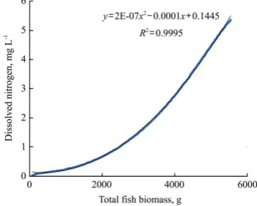
the aquaponics (Figure 12). The R2 value of 0.9995 was
presented in Figure 13, it showed the relationship
between dissolved nitrogen and fish biomass, suggesting
that AQUASMAT could be used to relate and quantify
nitrogen dynamics in a culture system.
Figure 11 Organic matter accumulation
Figure 12 TAN, NO3 and nitrogen input from feed in the system
Figure 13 Relationship between fish biomass and dissolved nitrogen in the system
In aquaponics, plants are grown in a hydroponic
system which enables them to use the nutrient-rich water
from the culture system. Nitrogen availability in fish
production systems is an important factor in determining
the success of an aquaponics system. The plants take up the nutrients, and then reduce or eliminate the water’s toxicity for the aquatic animal (Parker R., 2012).
According to Tyson (2012), 100 pounds of fish (45.5 kg)
will supply enough nitrogen for 4,050 lettuce plants or
540 tomato plants. Optimum feeding rate is 60-100 g of
fish feed m-2 of plant growing area/day (Shultz et al.,
2012) Simulation result from the farmer was used to
evaluate the possibility of integrating agriculture with
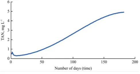
aquaculture (aquaponics). As shown in Figure 14-16, a
predicted fish biomass of 1 tonne (1000 kg), feeding rate
peak of about 300 g m-3 and accumulated ammonia was
observed. These results were in agreement with the
reports by Tucker and Ploeg (1993), and Hansen (1996).
They indicated that tomato, melon, pepper, lettuce and
cucumber nutrient requirement is approximately
0.08 mg L-1 d-1 to 0.16 mg L-1 d-1 nitrogen for growth,
flowering, fruiting. This result could be useful in gaining
insight into the nutrient generation needed for designing
the biofilter (grow bed) of an aquaponics system.
Figure 14 Predicted fish biomass
Figure 16 Predicted total ammonia nitrogen
4 Conclusion
In this study, the managerial and analytical capability
of the AQUASMAT was developed. The results predicted
the environmental quality, production and economic
outcomes of African catfish cultured in tanks in order to
aid stakeholders (farmers, managers, and researchers) in
carrying out production process (day-to-day management
operations such as determining stocking and feeding rates,
predicting dissolved oxygen levels and examining the
effects of different management strategies) and analyzing
economical ways of improving the productivity of their
farms. The result and process interrelationships
predicated in this model were in agreement with existing
literatures of water quality relationships. This result
indicated that the AQUASMAT model could be useful in
studying processes and interactions of water quality
parameters with respect to fish performance, and sizing of
biofilters for aquaponics systems.
References
Al-Hafedh, Y. S., A. Alam, and M. A. Alam. 2003. Performance of plastic biofilter media with different configuration in a water recirculation system for the culture of Nile tilapia (Oreochromis niloticus). Aquacultural Engineering, 29(3): 139–154.
Anyadike, C. C., C. C. Mbajiorgu, and G. N. Ajah. 2015. Aquacultural System Management Tool (AQUASMAT) I: Model development. Aquacultural Engineering, 69: 60–77. Boyd, C. E., and C. S. Tucker. 1998. Pond Aquaculture Water
Quality Management. Berlin, Germany: Springer Science and Business Media.
Ebeling, J. M. 2015. Water quality. Recirculting workshop on aquaculture systems technologies LLC Orleans L.A. Available at: www.ag.arizona.edu. Accessed 29 January 2016.
Hargreaves, J. A., and C. S. Tucker. 2003. Defining loading limits of static ponds for catfish aquaculture. Aquacultural Engineering, 28(1): 47–63.
Hargreaves, J. A., and J. R. Tomasso. 2004. Environmental biology. In: Developments in Aquaculture and Fisheries Science,
Biology and Culture of Channel Catfish. C. Tucker and J. Hargreaves, eds., 36-68. Netherlands: Elsevier B.V.
Hecht, T., W. Uys, and P. J. Britz. 1988. The culture of sharp tooth catfish, Clarias gariepinus in Southern Africa, In National Programs for Aquaculture Research, South African National Scientific Report, vol. 153: 47–61.
Isyagi, N. A., K. L. Veverica, R. Asiimwe, and W. H. Daniels. 2009. Manual for the Commercial Pond Production of the African Catfish in Uganda. 109–112. Kampala: Department of Fisheries and Allied Aquacultures; Alabama, USA: Auburn University.
Park, R., J. Carleton, J. Clough, and M. Wellman. 2009.
AQUATOX Technical Note 1: A Calibrated Parameter Set for Simulation of Algae in Shallow Rivers. Washington, DC: U.S. Environmental Protection Agency.
Park, R., and J. Clough. 2012. AQUATOX (Release 3.1) Technical Documentation vol.2. Washington, DC: U.S. Environmental Protection Agency.
Parker, R. 2012. Aquaculture Science. USA: Cengage Learning. Pillay, T. 2004. Aquaculture and the Environment. Oxford:
Blackwell Publishing.
Timmons, M. B., and J. M. Ebeling. 2010. Recirculating Aquaculture. Ithaca, NY: Cayuga Aqua Ventures.
Tucker, C. S. 1985. Organic matter, nitrogen, and phosphorus content of sediments from channel catfish ponds. Mississippi Agricultural and Forestry Experiment Station Research Report 10-7, Mississippi State University, Mississippi, USA. Tucker, C. S. 2000. Off-flavor problems in aquaculture. Critical
Reviews in Fisheries Science, 8(1): 45–88.
Tucker, C. S., J. Hargreaves, and C. Boyd. 2008. Aquaculture and the environment in the United States. In Environmental Best Management Practices for Aquaculture, 3-54. C. Tucker and J. Hargreaves, eds. Iowa: Blackwell Publishing.
Tucker, C. S., and M. Ploeg. 1993. Seasonal changes in water quality in commercial channel catfish ponds in Mississippi.
Journal of the World Aquaculture Society, 24(4): 473–481. Tyson, R. 2012. Aquaponics. University of Florida, Orange County
Extension Service. Available at: http://orange.ifas.ufl.edu/uf_workshop/pdffiles/Aquaponics%2 02012.pdf. Accessed 17 August 2012.