Cropping pattern optimization considering uncertainty of water
availability and water saving potential
Lina Hao
1,
Xiaoling Su
1*,
Vijay P. Singh
2(1. College of Water Resources and Architectural Engineering, Northwest A& F University, Yangling 712100, Shaanxi, China; 2. Department of Biological & Agricultural Engineering and Zachry Department of Civil Engineering, Texas A&M University,
College Station, TX 77843-2117, USA)
Abstract: In arid and semi-arid areas, the profitability of irrigated agriculture mainly depends on the availability of water resources and optimal cropping patterns of irrigation districts. In this study, an integrated agricultural cropping pattern optimization model was developed with considering the uncertainty of water availability and water saving potential in the future, aiming to maximize agricultural net benefit per unit of irrigation water. The available water which was based on the uncertainty of runoff was divided into five scenarios. The irrigation water-saving potential in the future was quantified by assuming an increase in the rate irrigation water-saving of 10% and 20%. The model was applied to the middle reaches of Heihe River basin, in Gansu Province, China. Results showed that if the irrigation water-saving rate was assumed to increase
by 10%, then the net water-saving quantity would increase by 21.5-22.5 million m3 and the gross water-saving quantity would
increase by 275.7-303.0 million m3. Similarly, if the irrigation water-saving rate increased by 20%, then the net water-saving
quantity would increase by 43.0-45.1 million m3 and the gross water-saving quantity would increase by 331.7-383.2 million m3.
If the agricultural cropping pattern was optimized, the optimal water and cultivated area allocation for maize would be greater than those for other crops. Under the premise that similar volume of irrigation water quantity was available in different scenarios, results showed differences in system benefit and net benefit per unit of irrigation water, for the distribution of available irrigation water was diverse in different irrigation districts.
Keywords: cropping pattern optimization, irrigation water-saving potential, different scenarios, water availability, water use efficiency, particle swarm optimization (PSO)
DOI: 10.25165/j.ijabe.20181101.3658
Citation:Hao L N, Su X L, Singh V P. Cropping pattern optimization considering uncertainty of water availability and water saving potential. Int J Agric & Biol Eng, 2018; 11(1): 178–186.
1 Introduction
Optimization of cropping patterns plays an important role in
high-benefit and water-saving agricultural management[1], which
determines the water requirement at the head and ultimately helps estimate the required capacity of the reservoir and the canal
system[2]. In arid and semi-arid areas, the profitability of irrigated
agriculture mainly depends on the availability of irrigation water and the cropping pattern of irrigation districts. Irrigation water is
a key determinant of a crop area optimization model[3]. However,
waste of irrigation water, owing to the lower use efficiency, has
made aggravated the crisis of irrigation water[4,5]. At present time
in northwest of China, irrigation efficiency is low, meaning there is
higher agriculture water-saving potential[6]. In order to alleviate
water shortage for irrigation, it is therefore essential to develop water-saving irrigation. Estimation of irrigation water-saving potential, which can calculate how much water could be saved by adopting water-saving measures, is desired and would benefit
Received date: 2017-07-22 Accepted date: 2017-11-28
Biographies: Lina Hao, PhD candidate, research interests: optimal allocation of water resources, Email: [email protected]; Vijay P. Singh, Professor, research interests: hydrology and hydraulics, Email: [email protected]. *Corresponding author: Xiaoling Su, Professor, research interests: optimal allocation of water resources, water conversion and regulation of water resources, College of Water Resources and Architectural Engineering, Northwest A&F University, No.23 Weihui Rd, Yangling 712100, Shaanxi, China. Tel: +86- 13892816132, Email: [email protected].
agricultural water management[7,8]. Many studies have
investigated water-saving potential[6,9,10]. Jägermeyr et al.[11]
incorporated a process-based irrigation system representation n into a bio-agrosphere model to calculate the water saving potential.
Yan et al.[12] investigated on-farm techniques to assess water
consumption of some crops. Gao et al.[13] applied user’s
preference for saving water and adopting end use analysis to
analyze water conservation. Damerau et al.[14] estimated water
saving potential from the viewpoint of development of future food and energy supply. However, previous literature focused on applying experimental and statistical methods to quantify agricultural water saving potential but relatively little attention was given to the irrigation water-saving potential caused by agricultural water-saving engineering development.
An optimal cropping pattern depends upon the water availability, with the objective of meeting the maximum irrigation
potential as well as the maximum economic return[2].
Mathematical models, such as linear programming[15-17] and
non-linear programming[7,18-20], have been widely used for
achieving different objectives. For cropping pattern optimization,
different optimization objectives, such as single objective[21] or
multi objectives[22,23] need to be considered for the decision maker.
For a multi objective model, mathematical techniques that can handle all the objectives simultaneously are needed. Examples of
such mathematical techniques include goal programming[24,25],
fuzzy optimization[26-28], and stochastic optimization[29-31].
optimization considering the influence of these factors. For
example, Zhang and Guo[8] obtained optimal solutions of planting
structure by adjusting planting scale and multiple cropping indexes to determine the rule of water saving quantity-benefit. Cid-Garcia
et al.[32] determined an optimal crop pattern for maximizing the
farmer’s expected profit by assessing the chemical and physical
management zones. Dong et al.[4] combined the vulnerability and
contribution rate assessment to propose an effective solution for crop structure adjustment.
However, incorporating the irrigation water-saving potential in cropping pattern optimization does not seem to have been investigated. Therefore, it would be desirable to develop a model that can handle uncertainties and complexities in cropping pattern optimization, with the aim to maximize profitability of irrigation water. This paper focuses on the irrigation water-saving potential, estimating how much water could be saved and reused in an irrigation system through the development of water-saving agriculture in future. Therefore this paper proposed a development pattern of agricultural crops in the future, based on agricultural cropping pattern optimization model considering different hydrological frequencies, and in conjunction with
agricultural irrigation water-saving potential in future.
2 Materials and methods
2.1 Study area
The study area is located in the middle reaches of Heihe River basin (97°37′-102°06′E, 37°44′ -42°40′N), northwest of China. In the arid and semi-arid areas, crop growth mainly depends on agricultural irrigation. Thus, agricultural available water should be taken into consideration, when making decision for suitable and
sustainable cultivated land scale[34]. However, it is estimated that
the water use efficiency of agricultural irrigation in the middle
reaches merely approaches to 0.52[3,5]. This suggests that there is
high agricultural water-saving potential. Improving the efficiency of irrigation water use thus becomes the effective way to improve
agricultural benefit[36]. Hence there is enormous potential to
improve agricultural water resources. Therefore, estimating irrigation water-saving potential, which can calculate how much water could be saved by adopting water-saving measures, is desired and would benefit water-saving agricultural development.
The study area includes 17 irrigation districts in Ganzhou District, Linze County and Gaotai County (as shown in Figure 1).
1. Luocheng irrigation district (LC) 2. Liuba irrigation district (LB) 3. Youlian irrigation district (YL) 4. Xinba irrigation district (XB) 5. Hongyazi irrigation district (HYZ) 6. Pingchuan irrigation district (PC) 7. Banqiao irrigation district (BQ) 8. Liaoquan irrigation district (LQ) 9. Yanuan irrigation district (YN) 10. Liyuanhe irrigation district (LYH) 11. Shahe irrigation district (SH) 12. Xijun irrigation district (XJ) 13. Yingke irrigation district (YK) 14. Daman irrigation district (DM) 15. Shangshan irrigation district (SS) 16. Huazhai irrigation district (HZ) 17. Anyang irrigation district (AY)
Figure 1 Study system of the middle reaches of Heihe River basin
2.2 Methods and data
2.2.1 Data acquisition
Data related to water-saving condition (water-saving area, irrigation quota in water-saving condition) were collected through Zhangye Irrigation Management Report (http://swj.zhangye. gov.cn/). Parameters related to irrigation quota, crop yield, the net irrigation quota of crop, cost and price of 7 crops were collected
through the Statistical Yearbook of Zhangye City
(http://www.zytj.gov.cn/). Agricultural price data were obtained from the Gansu prices net (http://www.gswj.gov.cn/). Annual minimum grain and vegetable demand were according to China Food and Nutrition Development Outline (http://www.moa. gov.cn/). Available irrigation water under different probabilities of water level in irrigation districts (as shown in Table 1) was
obtained from Zhao et al.[38]
The category of five flow year was based on the frequency
analysis method[38]. Let p denotes the hydrological frequencies,
the flow years divided into five conditions of very-high, high,
middle-level, low and very low with p≤12.5%, 12.5%<p≤37.5%,
37.5%<p≤62.5%, 62.5%<p≤87.5% and 87.5%<p, respectively.
2.2.2 Irrigation water-saving potential
In order to explore agricultural water-saving potential by adopting efficient agricultural water management inside an agriculture irrigation system, this study quantified agricultural water-saving potential by distinguishing “net water saving” and “gross water saving” based on irrigation water-saving potential
estimation theory[6] at the irrigation district scale under different
improving the efficiency of irrigation water use and reducing seepage loss and soil evaporation. The net water saving is the
quantity of saving of invalid water consumption and invalid loss water[6].
Table 1 Available irrigation water under different hydrological frequencies in irrigation districts million m3
Administrative region Irrigation districts Very-low years Low years Middle-level years High years Very-high years
Gaotai County
1 LC 36.14 36.05 35.82 35.72 35.64
2 LB 23.75 23.62 23.85 24.00 23.99
3 YL 253.31 241.87 236.00 231.94 230.81
4 XB 44.88 44.88 44.88 44.88 44.88
5 HYZ 22.03 22.03 22.03 22.03 22.03
6 PC 73.99 71.81 68.89 66.76 66.81
Linze County
7 BQ 89.96 76.15 71.62 66.87 66.98
8 LQ 33.82 33.81 33.12 32.87 32.89
9 YN 21.93 22.02 21.92 21.95 21.95
10 LYH 49.99 166.85 166.85 166.85 166.85
11 SH 39.34 34.56 32.90 31.66 33.44
Ganzhou District
12 XJ 234.21 224.93 216.94 211.95 221.52
13 YK 201.31 194.40 187.64 183.43 191.54
14 DM 169.35 168.92 164.12 161.18 167.03
15 SS 86.43 75.94 72.05 68.71 73.40
16 HZ 7.30 7.30 7.30 7.30 7.30
17 AY 26.68 26.68 26.68 26.68 26.68
Sum 1414.43 1471.82 1432.61 1404.77 1433.73
Figure 2 illustrates a detailed decomposition of gross water saving and net water saving. Gross water saving mainly includes two parts, one is invalid water loss reduced and the other is invalid water consumption reduced.
Figure 2 Components of gross water-saving quantity and net
water-saving quantity[6]
Gross water saving gives an account of engineering-type water-saving potential, which is the water saved in irrigation canal systems, field irrigation systems and management of water saving irrigation project. In other words, gross water saving is the amount of irrigation water saving on account of improving the efficiency of irrigation water use, which gives an account of the difference in value between irrigation water availability at the present time and water saving scenarios in future. According to the irrigation water-saving potential estimation theory established
by Lei et al.[6], net water-saving quantity and gross water-saving
quantity can be expressed as below. (1) Net water-saving quantity
The net water-saving quantity is defined as the saving quantity of invalid water consumption, expressed as Equation (1):
1
n
net i i
W A I
(1)where, ΔWnetis the net water-saving quantity; ΔAi is the increasing
area of water-saving measure i; and ΔIi is the reduction of net
irrigation quota of water-saving measure i.
(2) Gross water-saving quantity
Gross water-saving is the amount of water-saving on account of improving the efficiency of irrigation water use and reducing seepage loss and soil evaporation, expressed as Equation (2):
net 0 net gross 0 0
0
( t)
t
t
I I
W W W A
(2)
where, ΔWgross is the gross water-saving quantity; W0 is the
irrigation water in the status quo condition; Wt is the irrigation
water in the water-saving condition; A0is the irrigation area; Inet0is
the net irrigation quota in the status quo condition; Inettis the net
irrigation quota in the water-saving condition; η0is the efficiency
of water use in irrigation systems in the status quo condition; ηtis
the efficiency of water use in irrigation systems in the water-saving
condition. Here Inet0 can be formulated as Equation (3), Inett can
be formulated as Equation (4), ηt can be formulated as Equation (5),
ηi denotes the efficiency of water use of water-saving measure i.
0 0 0
0
net
W I
A
(3)
0 0
0
0 0
n
net i i
i net
nett net
A I A I
W
I I
A A
(4)
1 0
n
i i
i t
A
A
(5)2.2.3 Crop structure optimization model based on irrigation water-saving potential
seven main crops (maize, wheat, potato, maize seed, cotton, oil crops, and vegetables), which is in the pursuit of the maximum water use efficiency. The objective function of integrated agricultural cropping pattern optimization model can be expressed as follow equations:
7 7
1 1 1 1
max (( ) / ) /
n n
ij ij ij ij ij ij
i j i j
f y v c x ET x
(6)where, f is the expected net benefit per unit of irrigation water
(RMB/m3); i (i=1,2,…,17) is subarea, the meaning has been
illustrated in Table 1; j (j=1,2,…, 7) is the crop type, with j=1
means maize, j=2 wheat, j=3 means potato, j=4 means maize seed,
j=5 means cotton, j=6 means oil crops, j=7 means vegetables; xijis
decision variable, which expresses the planting area of crop j on
irrigation district i (ha); yijis the yield per unit area of crop j in the
irrigation district i (kg/ha); cij is the cost of crop j in the irrigation
district i (RMB/ha); and ETij is the net irrigation quota of crop j in
the irrigation district i (m3/hm2).
Subject to the following constraints:
Water supply to irrigation district would be less than the available water:
7
gross 1 1
n
ij ij i i
i j
m x Q W
(7)The crop area would be less then the irrigation district area:
7 1 1 n ij n i j x X
(8)Agricultural product (crop and vegetable) would be to meet the local demand: 4 1 1 n ij ij i j
x y K P FN
(9)1 9
n
ij ij i j
x y K P VN
(10)0 ij
x (11)
where, mij is the gross irrigation quota of crop j in the irrigation
district i (m3/hm2); Qi is the available water supply in the irrigation
district i (m3); ΔWgrossi is the gross water-saving quantity in the
irrigation district i (m3); Xn is the effective irrigated area of the
irrigation district i (hm2); P is the population in the study area; FN
is the per person grain demand, 135 kg/person; and VN is the per
person vegetable demand, 140 kg/person. 2.2.4 Particle swarm optimization
There are a large number of variables in the agricultural cropping pattern optimization model. Particle swarm optimization (PSO) is an effective alternative for dealing with multiple variables which is stochastic population-based algorithm motivated by intelligent collective behavior of birds.
In PSO, an individual is compared to a particle and the
population is called as a swarm[33]. The particle moves in a search
space by updating velocity and position which represent the possible way to the problem and the direction to obtain the global optimal value. The position and velocity can be upgraded by formulas (12) and (13):
1 1 2 2 g
( 1) ( ) ( ) ( ( ) ( )) ( ( ) ( ))
i i i i i
v t t v t c r P t x t c r P t x t
(12)
( 1) ( ) ( 1)
i i i
x t x t r v t (13)
where, vi(t) and xi(t) are the velocity and position of particle i at
iteration t; Pi(t) is the position with the best fitness value; Pg(t) is
the global best position; c1 and c2 are positive constant parameters
which are called acceleration coefficients, and are usually assigned
a value 1; r1, r2 are random numbers between 0 and 1; and ω
represents the inertia weight.
ω(t) can be upgraded according to the following formula[37]:
max max min max
( )t ( ) t t/
(14)
where, ωmax and ωmin are the maximum and minimum values of
inertia weight, and are usually assigned values of 1 and 0; and tmax
is the number of iterations.
Pi(t) and Pg(t) can be upgraded according to the following
formulas:
( 1), ( ( 1)) ( ( ))
( )
( ),
i i i
i
i
x t if fitness x t fitness x t p t
P t other wise
(15)
The optimal position of the whole swarm at time t is calculated
from Equation (11):
g( ) min ( ( )),1 ( ( )),2 , ( N( ))
P t fitness P t fitness P t fitness P t (16)
3 Results and discussion
The aim of model was to generate desired alternatives for crop area based on maximizing the net benefit per unit of irrigation water and given constraints. The model equations were solved using the method described in 2.2.4.
3.1 Irrigation water-saving potential
Irrigation water quantity is a key determinant of crop area optimization model. However, besides irrigation water, the irrigation water-saving potential in irrigation district can be used as irrigation water if engineering-type water-saving is considered.
The water-saving rate was represented as the relative proportion of water-saving irrigation area and effective irrigated area in this study. For the current situation, the effective irrigated
area is 140 349 hm2, and the water-saving irrigation area is
58 217 hm2, therefore the water-saving rate was 41.48%. The
water use efficiency is 0.52 in this region. The current condition
was defined as scenario S0. According to the water resources
planning of Zhangye City (http://www.zhangye.gov.cn/), the water use efficiency should exceed 0.60 by 2020. After the calculation in this paper, when the water-saving rate increased by 10% and 20%, it would increase to 0.6 and 0.62, which fulfills requirements of water resources planning. Therefore, the situations when water-saving rates increase 10% and 20% were defined as scenario
S1 and scenario S2 respectively.
Assuming the effective irrigated area 140 349 hm2 is invariable,
when the water-saving rate was assumed to increase 10%, the
increment of water-saving irrigation area would be 14 035 hm2.
However, when relative proportions of the canal water-saving irrigation area and field water-saving irrigation area exhibit randomness which will lead to highly uncertain water-saving quantity, because the reduction of net irrigation quota of field
water-saving irrigation was 1605 m3/hm2, while the reduction of
net irrigation quota of canal water-saving irrigation was
1530 m3/hm2. For example, in case the increment area was all
allocated to canal water-saving irrigation area, assuming the relative proportions between cannel leakage prevention and low pressure pipe transport is invariable, then the cannel leakage
prevention area should be 42 760 hm2 and the low pressure pipe
transport area should be 23 273 hm2. If the increment area was all
allocated to field water-saving irrigation area, then the area of cannel leakage prevention and low pressure pipe transport should
be the same as the area in S0 scenario. The water-saving area of
Based on the area analysis above, the water-saving potential was calculated according to the Equations (1)-(5), under the current
circumstance, gross irrigation quota is 13 096 m3/hm2, when
water-saving rate increases 10%, it would drop to 10 937-
11 132 m3/hm2, meanwhile net irrigation quota would drop from
6810 m3/hm2 to 6650-6657 m3/hm2. Accordingly, water use
efficiency would change from 0.520 to 0.598-0.608. Similarly,
when water-saving rate increases 20%, it would drop to 10 366-
10 733 m3/hm2, meanwhile net irrigation quota would drop to
6489- 6504 m3/hm2, accordingly, water use efficiency would rise to
0.606-0.626 (as shown in Table 3).
In order to solve the irrigation water-saving area in future, the maximum and minimum values of net water-saving quantity were calculated in order to mitigate the impact of uncertainty.
Table 2 Water-saving area under different water-saving scenarios
Scenario Water-saving rate/%
Effective irrigated area/hm2
Canal water-saving irrigation area/hm2 Field water-saving irrigation area/hm2
Total /hm2 Cannel leakage
prevention
Low pressure pipe
transport Drip irrigation Spray irrigation Other measures
S0 41.48 140349 33667 18328 6067 129 27 58217
S1 51.48 140349 33667-42760 18328-23273 6067-19747 129-420 27-87 72252
S2 61.48 140349 33667-51840 18328-28220 6067-33433 129-713 27-147 86287
Table 3 Water-saving potential under different water-saving scenarios
Scenario Gross irrigation quota /m3·hm-2
Net irrigation quota
/m3·hm-2 Water use efficiency
Net water-saving quantity /million·m-3
Gross water-saving quantity /million·m-3
S0 13096 6810 0.520
S1 10 937-11 132 6650-6657 0.598-0.608 21.5-22.5 275.7-303.0
S2 10 366-10 733 6489-6504 0.606-0.626 43.0- 45.1 331.7-383.2
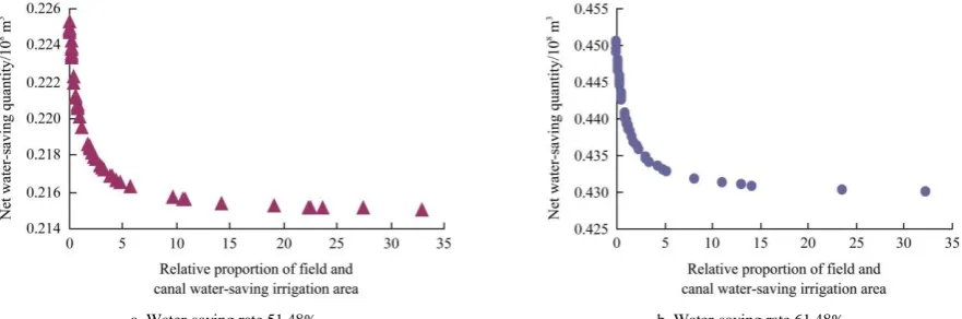
Figure 3 shows the relationship between net water-saving quantity and relative proportions of canal water-saving irrigation area and field water-saving irrigation area. In case the increment area was all allocated to canal water-saving irrigation area, the net
water-saving quantity would be 21.5 million m3. Otherwise, in a
situation in which the increment area was all allocated to field water-saving irrigation area, the net water-saving quantity would be
22.5 million m3. Namely, if water-saving rate increases by 10%,
the net water-saving quantity would increase by 21.5-22.5 million m3,
the gross water-saving quantity would increase by 275.7-
303.0 million m3. Similarly, if the water-saving rate increased by
20%, the net water-saving quantity would increase by 43.0-
45.1 million m3, the gross water-saving quantity would increase by
331.7-383.2 million m3.
a. Water-saving rate 51.48% b. Water-saving rate 61.48%
Figure 3 Net water-saving quantity under different water-saving rate
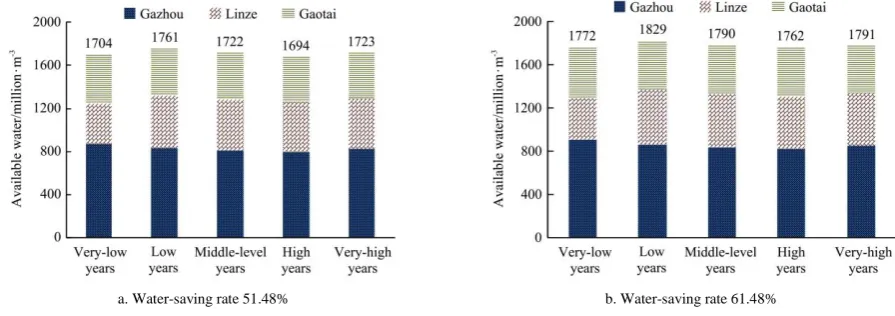
3.2 Available irrigation water
A development pattern of agricultural crop structure in the future was proposed by considering an agricultural cropping pattern optimization model under different probabilities of water level, and in conjunction with agricultural water saving potential in future. Figure 4 shows the available irrigation water when water-saving rate increases 10% and 20%. In Heihe River basin, State Council of the People's Republic of China introduced a series of regulations about water reallocation of the Heihe River to recover ecological environment in the downstream area and relieve water contradiction in Heihe River basin. The plan of water reallocation of the Heihe River stipulates the water discharge of Zhengyixia station under different probabilities of water level, for example, when the probability of water level is 90%, stream flow in
Yingluoxia station is 1900 million m3, there must be 1320 million m3
discharge at Zhengyixia station. However, when the probability of water level is 10%, stream flow in Yingluoxia Station is
1290 million m3, there must be 630 million m3 discharges at
Zhengyixia station. Therefore, the available water for agriculture will become less in high flow year compared with the low flow year.
3.3 Cropping pattern optimization
According to various flow levels and agricultural water saving potential, 7 different crops and 10 scenarios of water availability were designed to analyze agricultural cropping patterns in future. Scenarios 1 and 2 are in very-low years, the water-saving rates are 51.48% and 61.48%, respectively, and the available water volumes
for agriculture are 1704 million m3 and 1772 million m3; scenarios
agriculture are 1761 million m3 and 1829 million m3; scenarios 5 and 6 are in normal flow years, the water-saving rates are 51.48% and 61.48% respectively, and the available water volumes for
agriculture are 1722 million m3 and 1790 million m3; scenario 7
and 8 are in high flow years, the water-saving rates are 51.48% and
61.48%, respectively, and the available water volumes for
agriculture are 1694 million m3 and 1762 million m3; and scenarios
9 and 10 are in very-high flow years, the water-saving rates are 51.48% and 61.48%, respectively, and the available water for
agriculture are 1723 million m3 and1791 million m3.
a. Water-saving rate 51.48% b. Water-saving rate 61.48%
Figure 4 Available irrigation water under different water-saving rate
Figure 5 presents the optimized crop area patterns in different scenarios of Ganzhou, Linze and Gaotai County. In conjunction with available irrigation obtained from Figure 4, the total cultivated areas were different, because of the different available water under different scenarios.
The process of determining the optimal cropping pattern was operating at the level of irrigation district. In fact, optimal solutions of planting structure were related to various variables, such as irrigation quota and yield per hectare, which were different in different irrigation districts. Figure 5a gives the optimal cropping pattern under very low flow level. In Figure 5a, as water-saving rate increases under the same water level, the cultivable area of maize seed increases in Ganzhou, Linze and Gaotai county, while the vegetable and potato area is transferred to other 5 crops in Ganzhou county, the wheat and potato area is transferred to other 5 crops in Linze county, and the wheat area is transferred to other 6 crops in Gaotai county.
It can be found in Figure 5 and Table 4 that the cultivable area of maize seed and the optimal system benefit increases in Ganzhou, Linze and Gaotai county, while the total quantity of irrigation water increases. That means the optimal water and cultivated area allocation to maize seed is greater than water and cultivated area allocation to other crops. For the reason that compares with other crops, the irrigation quota of maize seed is smaller than maize, potato and vegetable in most irrigation districts and the unit price is higher than maize, wheat, potato and vegetable in most irrigation districts, so that the benefit per unit of water is higher than other crops.
Another relevant result is the fact that the major crops in Ganzhou, Linze and Gaotai county are similar, while the proportions of the main crops are different in these three counties. For example, the proportion of maize seed in Ganzhou, Linze and Gaotai County is about 77%, 59%, 40% respectively. Except for maize seed, the cultivable area of maize area is the second largest in Ganzhou county, accounting for about 10% in different scenarios, and then is vegetable and wheat, accounting for about 7% and 5%, respectively.
While the cultivable area of wheat is the second largest in Linze County, approaching 26% in different scenarios, and then is vegetable and maize, the proportions of them are nearly 9% and 6%, respectively. However, the cultivable area of maize is the second
largest in Gaotai County, accounting for approximately 23% in different scenarios, and then is vegetable and cotton; the proportions of them are nearly 14% and 12%, respectively.
Comparing Figure 5c with Figure 5e, it can be found that the total quantities of irrigation water are approximate under normal flow level and very-high flow level, however, the optimized crop area patterns showed some differences, for the available irrigation water allocation is different in irrigation districts.
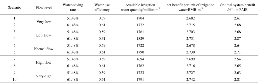
The solutions obtained can not only provide an effective evaluation under present scenarios, but also reveal the associated economic implications. Different scenarios would result in varied system benefits. Table 4 gives the system benefits of the middle reaches of Heihe River basin under different scenarios. Results reveal that stream flow level is an important variable which can directly affect optimal system benefit.
Under the premise of maximum economic benefit per unit of irrigation water, optimal total benefit achieves 2.68 billion RMB,
and the benefit of per unit of irrigation water is 2.703 RMB/m3
under low flow level, with the available irrigation water quantity
being 1761 million m3 and the water-saving rate being 51.48%,
when the water-saving rate increases to 61.48%, optimal total benefit would achieve 2.87 billion RMB, and benefit of per unit of
irrigation water would be 2.731 RMB/m3.
It reveals under the same distribution of available irrigation water that as the quantity decreases, the system benefit and net benefit per unit of irrigation water would decrease for the reason of less water availability. For example, optimal total benefit achieves 2.54 billion RMB, and benefit of per unit of irrigation
water is 2.699 RMB/m3 under high flow level, with available
irrigation water quantity being 1694 million m3 and water-saving
rate being 51.48%, when the water-saving rate increases to 61.48%, optimal total benefit would achieve 2.65 billion RMB, and benefit
of per unit of irrigation water would be 2.716 RMB/m3.
a. Very-low years b. Low years
c. Middle-level years d. High years
e. Very-high years
Note: The inner circle presents water-saving rate is 51.48%; the outer circle presents water-saving rate is 61.48%.
Table 4 Optimal system benefit under different water-saving scenarios
Scenario Flow level Water-saving rate
Water use efficiency
Available irrigation water quantity/million m3
net benefit per unit of irrigation water/RMB·m-3
Optimal system benefit /billion RMB 1
Very-low 51.48% 0.59 1704 2.682 2.61
2 61.48% 0.61 1772 2.715 2.68
3
Low flow 51.48% 0.59 1761 2.703 2.68
4 61.48% 0.61 1829 2.731 2.87
5
Normal flow 51.48% 0.59 1722 2.678 2.64
6 61.48% 0.61 1790 2.730 2.71
7
High flow 51.48% 0.59 1694 2.699 2.54
8 61.48% 0.61 1762 2.716 2.65
9
Very-high
51.48% 0.59 1723 2.727 2.63
10 61.48% 0.61 1791 2.742 2.81
4 Conclusions
The development pattern of agricultural crops structure in the future was proposed by considering an agriculture cropping pattern optimization model under different probabilities of water levels, and in conjunction with agricultural water-saving potential in future and was applied to Heihe River basin in Gansu Province, China.
This model is based on quantifying agricultural water-saving potential and determining the optimal structure which could obtain maximum agricultural net benefit per unit of irrigation water by allocating the limited water to 7 main crops. The main advantage of this model is that it can quantify the water-saving potential of irrigation area in future by calculating the maximum and minimum values of net water-saving quantity.
Under the premise of water-saving agricultural irrigation development, there is enormous water-saving potential in the middle reaches of Heihe River basin. Under the current
circumstance the gross irrigation quota is 13 096 m3/hm2, when the
water-saving rate increases by 10%, it would drop to 10 937-
11 132 m3/hm2, accordingly, the water use efficiency would change
from 0.520 to 0.598-0.608. As a result, there would be 275.7-
303.0 million m3 irrigation water to be saved. Similarly, when
water-saving rate increases by 20%, there would be 331.7-
383.2 million m3 irrigation water to be saved.
Seven different crops and 10 scenarios of water availability have been designed to analyze the different agriculture cropping patterns in future according to various flow levels and agriculture water saving potential, aiming at maximizing the profitability of irrigation agriculture by incorporating a more efficient use of irrigation water through effective crop structure adjustment. It suggests that the optimal water and cultivated area allocation to maize seed is greater than to other crops. The irrigation quota of maize seed is smaller than maize, potato and vegetable in most irrigation districts and its unit price is higher than maize, wheat, potato and vegetable in most irrigation districts, so that the benefit per unit water is higher than other crops.
Under the premise of similar volume of irrigation water quantity available in different scenarios, results show the difference in system benefit and net benefit per unit of irrigation water, for the distribution of available irrigation water is diverse in different irrigation districts.
Acknowledgments
We acknowledge that this work was financially supported by the National Natural Science Fund in China (Grant No. 91425302,
91325201) and National Key Research and Development Program during the 13th Five-year Plan in China (Grant No. 2016YFC0401306).
[References]
[1] Niu G, Li Y P, Huang G H, Liu J, Fan Y R. Crop planning and water resource allocation for sustainable development of an irrigation region in China under multiple uncertainties. Agricultural Water Management, 2016; 166: 53–69.
[2] Rai R K, Singh V P, Upadhyay A. Planning and evaluation of irrigation projects. Academic Press, 2017.
[3] Su X L, Li J F, Singh V P. Optimal allocation of agricultural water resources based on virtual water subdivision in Shiyang River Basin. Water Resources Management, 2014; 28(8): 2243–2257.
[4] Dong Z Q, Pan Z H, Wang S, An P L, Zhang J T, Zhang J, et al. Effective crop structure adjustment under climate change. Ecological Indicators, 2016; 69: 571–577.
[5] Asres S B. Evaluating and enhancing irrigation water management in the upper Blue Nile basin, Ethiopia: The case of Koga large scale irrigation scheme. Agricultural Water Management, 2016; 170: 26–35.
[6] Lei B, Liu Y, Xu D. Estimating theory and method of irrigation water-saving potential based on irrigation district scale. Transactions of the CSAE, 2011; 27(1): 10–14. (In Chinese)
[7] López-Mata E, Orengo-Valverde J J, Tarjuelo J M, Martinez-Romero A, Dominguez A. Development of a direct-solution algorithm for determining the optimal crop planning of farms using deficit irrigation. Agricultural Water Management, 2016; 171: 173–187.
[8] Zhang D, Guo P. Integrated agriculture water management optimization model for water saving potential analysis. Agricultural Water Management, 2016; 170: 5-19.
[9] Karimov A, Molden D, Khamzina T, Platonov A, Ivanov Y. A water accounting procedure to determine the water savings potential of the Fergana Valley. Agricultural water management, 2012; 108: 61–72. [10] Törnqvist R, Jarsjö J. Water savings through improved irrigation
techniques: basin-scale quantification in semi-arid environments. Water Resources Management, 2012; 26(4): 949–962.
[11] Jägermeyr J, Gerten D, Heinke J, Schaphoff S, Matti K, Lucht W. Water savings potentials of irrigation systems: global simulation of processes and linkages. Hydrology and Earth System Sciences, 2015; 19(7): 3073-3091. [12] Yan N N, Wu B F, Perry C, Zeng H W. Assessing potential water savings in agriculture on the Hai Basin plain, China. Agricultural Water Management, 2015; 154: 11–19.
[13] Gao H C, Wei T, Lou I, Yang Z F, Shen Z Y, Li Y X. Water saving effect on integrated water resource management. Resources, Conservation and Recycling, 2014; 93: 50–58.
[14] Damerau K, Patt A G, van Vliet O P R. Water saving potentials and possible trade-offs for future food and energy supply. Global Environmental Change, 2016; 39: 15–25.
[15] Zeng X T, Kang S Z, Li F S, Zhang L, Guo P. Fuzzy multi-objective linear programming applying to crop area planning. Agricultural Water Management, 2010; 98(1): 134–142.
[17] Galán-Martin A, Pozo C, Guillén-Gosálbez G, Vallejo A A, Esteller L J. Multi-stage linear programming model for optimizing cropping plan decisions under the new Common Agricultural Policy. Land Use Policy, 2015; 48: 515–524.
[18] Garg N K, Dadhich S M. Integrated non-linear model for optimal cropping pattern and irrigation scheduling under deficit irrigation. Agricultural Water Management, 2014; 140: 1–13.
[19] Liu H, Wang X, Zhang X, Zhang L W, Li Y, Huang G H. Evaluation on the responses of maize (Zea mays L.) growth, yield and water use efficiency to drip irrigation water under mulch condition in the Hetao irrigation District of China. Agricultural Water Management, 2017; 179: 144–157.
[20] Singh A, Panda S N. Development and application of an optimization model for the maximization of net agricultural return. Agricultural Water Management, 2012; 115: 267–275.
[21] Pant M, Thangaraj R, Rani D, Abraham A, Srivastava D K. Estimation of optimal crop plan using nature inspired metaheuristics. World Journal of Modeling and Simulation, 2010; 6(2): 97–109.
[22] Sarker R, Ray T. An improved evolutionary algorithm for solving multi-objective crop planning models. Computers and Electronics in Agriculture, 2009; 68(2): 191–199.
[23] Márquez A L, Baños R, Gil C, Montoya M G, Manzano-Agugliaro F, Montoya F G. Multi-objective crop planning using pareto-based evolutionary algorithms. Agricultural Economics, 2011; 42(6): 649–656. [24] Prisenk J, Turk J. A multi-goal mathematical approach for the
optimization of crop planning on organic farms: a Slovenian case study. Pakistan Journal of Agricultural Sciences, 2015; 52(4): 971–979.
[25] Srivastava P, Singh R M. Optimization of cropping pattern in a canal command area using fuzzy programming approach. Water Resources Management, 2015; 29(12): 4481–4500.
[26] Sharma D K, Jana R K. Fuzzy goal programming based genetic algorithm approach to nutrient management for rice crop planning. International Journal of Production Economics, 2009; 121(1): 224–232.
[27] Lu H W, Huang G H, He L. Development of an interval-valued fuzzy linear-programming method based on infinite α-cuts for water resources management. Environmental Modelling & Software, 2010; 25(3):
354–361.
[28] Yang G Q, Guo P, Huo L J, Ren C F. Optimization of the irrigation water resources for Shijin irrigation district in north China. Agricultural Water Management, 2015; 158: 82–98.
[29] Xie Y L, Huang G H, Li W, Li J B, Li Y F. An inexact two-stage stochastic programming model for water resources management in Nansihu Lake Basin, China. Journal of Environmental Management, 2013; 127: 188–205.
[30] Li M, Guo P. A coupled random fuzzy two-stage programming model for crop area optimization—A case study of the middle Heihe River basin, China. Agricultural Water Management, 2015; 155: 53–66.
[31] Stoyan S J, Kwon R H. A two-stage stochastic mixed-integer programming approach to the index tracking problem. Optimization and Engineering, 2010; 11(2): 247–275.
[32] Cid-Garcia N M, Bravo-Lozano A G, Rios-Solis Y A. A crop planning and real-time irrigation method based on site-specific management zones and linear programming. Computers and Electronics in Agriculture, 2014; 107: 20–28.
[33] Kennedy J. Particle swarm optimization. Encyclopedia of Machine Learning. Springer US, 2011.
[34] Su X L, Singh V P, Niu J P, Hao L N. Spatiotemporal trends of aridity index in Shiyang River basin of northwest China. Stochastic Environmental Research and Risk Assessment, 2015; 29(6): 1571–1582. [35] Li X L, Tong L, Niu J, Kang S Z, Du T S, Li S E, et al. Spatio-temporal
distribution of irrigation water productivity and its driving factors for cereal crops in Hexi Corridor, Northwest China. Agricultural Water Management, 2017; 179: 55–63.
[36] Tong F F, Guo P. Simulation and optimization for crop water allocation based on crop water production functions and climate factor under uncertainty. Applied Mathematical Modeling, 2013; 37(14): 7708–7716. [37] Clerc M, Kennedy J. The particle swarm-explosion, stability, and
convergence in a multidimensional complex space. IEEE Transactions on Evolutionary Computation, 2002; 6(1): 58–73.
![Figure 2 Components of gross water-saving quantity and net water-saving quantity[6]](https://thumb-us.123doks.com/thumbv2/123dok_us/595775.2058878/3.595.42.556.109.365/figure-components-gross-water-saving-quantity-saving-quantity.webp)