Deterministic nature of the underlying dynamics of surface wind fluctuations

www.ann-geophys.net/30/1503/2012/ doi:10.5194/angeo-30-1503-2012

© Author(s) 2012. CC Attribution 3.0 License.

Annales

Geophysicae

Deterministic nature of the underlying dynamics of surface wind

fluctuations

R. C. Sreelekshmi1, K. Asokan2, and K. Satheesh Kumar1

1_{Department of Futures Studies, University of Kerala, Thiruvananthapuram, Kerala, 695 034, India} 2_{Department of Mathematics, College of Engineering, Thiruvananthapuram, Kerala, 695 016, India} Correspondence to: K. Satheesh Kumar ([email protected])

Received: 14 March 2012 – Revised: 6 August 2012 – Accepted: 3 September 2012 – Published: 8 October 2012

Abstract. Modelling the fluctuations of the Earth’s surface

wind has a significant role in understanding the dynamics of atmosphere besides its impact on various fields ranging from agriculture to structural engineering. Most of the studies on the modelling and prediction of wind speed and power re-ported in the literature are based on statistical methods or the probabilistic distribution of the wind speed data. In this pa-per we investigate the suitability of a deterministic model to represent the wind speed fluctuations by employing tools of nonlinear dynamics. We have carried out a detailed nonlin-ear time series analysis of the daily mean wind speed data measured at Thiruvananthapuram (8.483◦N,76.950◦E) from 2000 to 2010. The results of the analysis strongly suggest that the underlying dynamics is deterministic, low-dimensional and chaotic suggesting the possibility of accurate short-term prediction. As most of the chaotic systems are confined to laboratories, this is another example of a naturally occurring time series showing chaotic behaviour.

Keywords. Atmospheric composition and structure

(Gen-eral or miscellaneous)

1 Introduction

Surface wind plays a crucial role in climate and weather sys-tem of the Earth. It has significant impact on agriculture, nav-igation, structural engineering calculations and reduction of atmospheric pollution as well as the economy of the region as an alternate energy source (Mart´ın et al., 1999; Elliott, 2004; Bantaa et al., 2011; Finzi et al., 1984). Recent surge of interest in research related to wind power is due to its po-tential as an alternate source of energy because of the fast depletion of natural resources of Earth. Presently, there is

extensive literature on various areas related to wind energy acquisition and utilisation such as wind speed modelling and prediction, wind power production and wind resource quan-tification (e.g. Finzi et al., 1984; Mart´ın et al., 1999; Elliott, 2004; Celik, 2004; von Bremen, 2007; Mabel and Fernan-dez, 2009; Kavasseri and Seetharaman, 2009; Bantaa et al., 2011).

Wind speed modelling and forecasting is an important as-pect of wind power generation – yet one of the most diffi-cult due to the myriads of factors affecting it – and over the years many tools have been developed for this purpose. A good number of such tools rely on statistical methods, either moving average models such as ARMA and ARIMA fitted to the time series of wind speed (Kamal and Jafri, 1997; Tor-resa et al., 2005; Cadenas and Rivera, 2007; Kavasseri and Seetharaman, 2009) or models based on probability distribu-tion of wind speed (Hennessey, 1977; Celik, 2004; Mathew et al., 2011). Models based on artificial neural networks have also been developed by many authors for making short-term predictions of wind speed and generated wind power (Mo-handes et al., 1998; Cadenas and Rivera, 2007; Bilgili et al., 2007; Monfared et al., 2009).

the dynamics, rather on comparing stochastic versus deter-ministic models constructed from time series of scalar mea-surements of wind speed. Palmer et al. (1995) have analysed several time series of wind components and X-band Doppler radar signals gathered over an area of ocean surface and have found the presence of a low-dimensional dynamical attractor in the case of time series of the horizontal wind speed as well as the vertically polarized radar reflectivity. They were also able to achieve better short-term predictions from the deter-ministic models than from statistical models. However, the analysis carried out on daily mean wind speed (DMWS) data by Ragwitz et al. (2000) suggests that, on average, no reduc-tion of the predicreduc-tion error can be achieved by using a nonlin-ear model instead of a linnonlin-ear stochastic model. However, they could predict intermittent gusts with significantly higher ac-curacy. These studies are however limited by short times se-ries (Hirata et al., 2008). Mart´ın et al. (1999) have analysed the wind speed data by splitting them into deterministic and stochastic components. Their analysis shows that the deter-ministic component has 1-year, 24-h and 12-h periods. These cycles have also been observed by other authors in surface wind studies (Brett and Tuller, 1991; Gavald´a et al., 1992). The 1-year and 24-h periods are the natural Earth cycles. The 12-h period for wind speed series is well-defined and cor-responds to the daytime and nighttime maxima due to the full development of the land–sea breezes. These periodicities present in the wind speed time series clearly show presence of determinism in the data. However, it is not clear whether the apparent stochastic component is strictly stochastic or arises out of chaotic underlying dynamics.

In general, the predictability and degree of determinism of atmospheric parameters depend on the time scale con-sidered (Palmer, 1993), and this applies in particular to the case of wind speed predictions. The various models for wind speed predictions reviewed above are mostly in time scales ranging from hours to a few days. What follows from this discussion is that wind is believed to have both determin-istic and stochastic components in the time scales consid-ered, but the manner in which these components interact is still elusive and a matter of debate. The rotation of Earth and solar heat radiation are two major causes of the sur-face wind in addition to the local topography. The Earth’s revolution is clearly deterministic. However, many authors have argued that the solar radiations are stochastic in na-ture and hence the underlying dynamics of the surface wind should be governed by both deterministic as well as stochas-tic factors. On the other hand, our previous analysis of the data of total electron content (TEC), which is strongly influ-enced by the solar radiation, shows strong evidence of de-terministic low-dimensional character of the underlying dy-namics (George et al., 2002; Kumar et al., 2004). The sur-face wind speed is a similar atmospheric parameter to so-lar influence but its dynamics is further complicated by the local conditions such as topography. Hence, it is worth in-vestigating whether a stochastic or a deterministic model is

most suitable for the underlying dynamics of surface wind fluctuations. In this work we carry out a detailed system-atic analysis of the time series of daily mean wind speed (DMWS) measured at Thiruvananthapuram, Kerala, India (8.483◦N,76.950◦E ; elevation: 64 m) using tools of nonlin-ear dynamics for the period from ynonlin-ear 2000 to 2010. Note that the length of the time series is about the length of a solar cycle. The data were obtained from National Climatic Data Centre (http://www.ncdc.noaa.gov). We demonstrate, using the DMWS-data, that the dynamics of wind speed is essen-tially deterministic with a low-dimensional chaotic charac-ter. The chaotic behaviour is what makes the long-term pre-dictions of wind speed erroneous, but it should be possible to obtain better short-term predictions using the determinis-tic model than would otherwise be made with the statisdeterminis-tical methods. It is reported that short-term predictions of one to six hours ahead at intervals of 10 min are important in power dispatching systems (Mabel and Fernandez, 2009).

We assume that there is also a stochastic component in the data arising mainly from measurement and averaging er-rors. The averaging errors are a result of considering the mean wind speeds and not the actual wind speeds equidis-tant in time as it should be for a time series. The effects of these errors are assumed to contribute an additive noise to the data which is independent of the true deterministic dy-namics of the system. Hence, the first step in our analysis is to remove the effect of this noise process using a suitable noise reduction technique to reveal the true dynamics behind the data. The denoised data still contain irregular persistent fluctuations, which upon analysis using tools of non-linear dynamics reveals many attributes of a chaotic system with a low-dimensional attractor. Since some of these attributes may also be found in linear stochastic processes, we further subject the denoised data to a detailed surrogate analysis to confirm that the underlying dynamics is indeed deterministic and could not be described by a linear Gaussian stochastic model. Most of these analyses were carried out using tools implemented in the TISEAN package (Hegger et al., 1999).

2 Time delay coordinates and attractor reconstruction

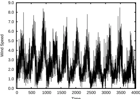
0.0 1.0 2.0 3.0 4.0 5.0 6.0 7.0 8.0 9.0

0 500 1000 1500 2000 2500 3000 3500 4000

Wind Speed

Time

Fig. 1. Time series of the measured daily mean wind speed (DMWS) in knots.

described by a state vectorx(t )and an equation of motion:

˙ x≡dx

dt =f (x). (1)

Such systems are usually characterised by an attractor, which is a bounded subset of the phase space reached asymptoti-cally by a set of trajectories over an open set of initial condi-tions as timet→ ∞.

A striking feature of some dynamical systems is that the trajectories on the attractor may exhibit sensitive dependence on initial conditions. This means that trajectories starting from neighbouring initial conditions may separate from each other at an exponential rate, evolving independently of each other and in an apparently uncorrelated manner after a suf-ficiently long period of time, and yet remain confined to a bounded subset of the phase space. Chaos is the bounded aperiodic behaviour in a deterministic system that shows sensitive dependence on initial conditions (Alligood et al., 1997). A detailed illustration of the sensitivity to initial con-ditions of a chaotic system, particularly in the setting of at-mospheric prediction, has been presented by Palmer (1993). The term chaos is reminiscent of the intricate dynamics ex-perienced by the trajectories on the attractor; the exponential divergence stretches out the trajectories as it evolves in time, which is then folded back to remain confined to a finite re-gion of the phase space. The attractor is the result of these sequences of stretching and folding repeated indefinitely.

Exponential divergence of trajectories on the attractor makes long-term predictions in a chaotic system difficult while the stretching and folding of trajectories cause mea-surements of quantities that depend on the state space to look random. Together, these attributes often make a chaotic sys-tem indistinguishable from a truly stochastic syssys-tem. In fact, many systems that were earlier dubbed as stochastic were later shown to be chaotic (Alligood et al., 1997; Ott, 1993).

Most of the time the state vectorx(t )is not measured di-rectly but indidi-rectly at discrete time intervalsτ using a scalar measurement functiony(t )=h(x(t ))leading to a time series yi =y(iτ ). The central idea in time series analysis is that the dynamics of the state vectorx(t )on the attractor can be re-captured from the time seriesy(t )using a technique called attractor reconstruction, first suggested by Packard et al. (1980) and successfully used by many others. This technique is based on the fact that the dynamics of then-dimensional state vectorx(t )on the attractor is topologically identical to that of them-dimensional delay vector:

y(t)=(y(t ), y(t+τ ),· · ·y(t+(m−1)τ ), (2) which was constructed from samples ofy(t )taken at regu-lar time intervalsτ (also called “delay”), under the mapping

x(t )−→y(t)which is an embedding under rather general conditions. The embedding theorem of Takens (1981) and its extensions (Sauer et al., 1991; Sauer and Yorke, 1993) furnishes the mathematical theory behind reconstruction and asserts that the embedding is valid for almost all values of time delay τ and all smooth measurement functions h as long asm >2DwhereDis the box-counting dimension of the attractor. This means that the dynamical and geometrical characteristics of the original system, in particular the geo-metrical invariants such as the fractal dimension, Lyapunov exponents and entropies, are preserved in the reconstructed space and can be computed from the flow defined byy(t ) (Kantz and Schreiber, 1997; Ott et al., 1994). The analysis of the DMWS-data, presented in the next section, relies on attractor reconstruction for computing many such character-istics.

3 Analysis of the denoised data

For the purpose of our analysis of the DMWS-data, we heuristically assume that the dynamics underlying wind can be modelled by a deterministic system with state vectorx(t ). The daily mean wind speed can be regarded as observations of a measurement function y(t )=h(x(t )) made at regular intervals. However, since we are considering the mean wind speeds and not the actual wind speeds at regular daily inter-vals, regarding them as observations made at equal intervals of time contributes an averaging error. We assume that these averaging errors along with other measurement errors can to-gether be modelled as an additive noise process with zero average and delta correlation. It is therefore important to re-duce the effect of this noise before analysing the data. For reducing noise we have applied the noise reduction method of Schreiber (1993), which employs a locally constant ap-proximation of the dynamics to reduce noise.

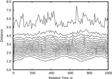
0.0 1.0 2.0 3.0 4.0 5.0 6.0 7.0 8.0 9.0

0 500 1000 1500 2000

Distance

Relative Time Δt

Fig. 2. Space-time separation plot for the time series in Fig. 1 for τ=1 andm=14.

temporal correlations inside the time series (Provenzale et al., 1992). Each point in the plot represents a pair of points on the trajectory with their relative separation in time along the horizontal axis and separation in space along the verti-cal. Marked variations are observed in the graph at multiples of around 365 days indicating annual variations. The mod-ulation effects due to these annual variations were reduced in subsequent analysis by applying epoch analysis on the data, by deducting from each of the data points which are 365 days apart their average value (Kumar et al., 2004). The resulting time series showed prominent variations, in periods of 28 days, arising from lunar influence. Hence, epoch anal-ysis was repeated for these 28-day variations as well. The plot of the resultant denoised and detrended time series is shown in Fig. 3 and its space-time separation plot in Fig. 4 which clearly show considerable reduction in the effect of the annual and lunar variations. The autocorrelation function (Eq. 3, discussed later) of the observed time series is plotted in Fig. 5a and of the detrended time series in Fig. 5b which also show that the temporal correlation due to the annual vari-ation and lunar influence has significantly been reduced by the epoch analysis. As is clear from the Fig. 3, the denoised detrended data still show persistent temporal fluctuations.

As a first step in the analysis of the denoised data, we de-termine the embedding parameters – the delayτ and the em-bedding dimensionm– for the proper reconstruction of the attractor using the method discussed in the previous section. The embedding theorems do not place any restriction what-soever on the delayτ and the embedding dimensionm, but their choice can nonetheless affect the inferences deduced from reconstruction significantly, especially when the data come from experiment. Small delays, for example, result in highly correlated vectorsy(t )leading to unduly larger val-ues for the correlation dimension, while large delays yield vectors with fairly uncorrelated components resulting in data randomly distributed in the embedding space (Kantz and

-5.0 -4.0 -3.0 -2.0 -1.0 0.0 1.0 2.0 3.0 4.0 5.0

0 500 1000 1500 2000 2500 3000 3500 4000

Wind Speed

Time

Fig. 3. Time series of the detrended denoised daily mean wind

speed shown in Fig. 1.

0.0 1.0 2.0 3.0 4.0 5.0 6.0 7.0 8.0

0 200 400 600 800 1000

Distance

Relative Time Δt

Fig. 4. Space-time separation plot for the detrended time series for τ=1 andm=14.

Schreiber, 1997). Proper choice of the time delay is, there-fore, important, and a first guess of a suitable delay may be obtained from the autocorrelation function of the sample data yi given by

ρ(τ )=

P

i(yi− ¯y)(yi+τ− ¯y) P

i(yi− ¯y)2

(3)

wherey¯is the sample mean. The value ofτ, at which the au-tocorrelation attains its first zero or its first local minimum, is usually an optimal choice for the delay (Kantz and Schreiber, 1997).

-0.4 -0.2 0.0 0.2 0.4 0.6 0.8 1.0

0.0 50.0 100.0 150.0 200.0

Autocorrelation

Delay (a)

0 0.2 0.4 0.6 0.8 1

0 10 20 30 40 50

Autocorrelation

Delay (b)

Fig. 5. (a) The autocorrelation function of the observed DMWS

data. (b) The autocorrelation function of the detrended time series.

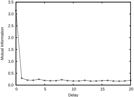
0.0 0.5 1.0 1.5 2.0 2.5 3.0 3.5

0 5 10 15 20

Mutual Information

Delay

Fig. 6. Mutual information of the time series of the measured

DMWS data.

regarding the sequences(yi)and(yi+τ)as values of random variablesXandY and using the formula

I (τ )=X

y∈Y X

x∈X

p(x, y)log₂

p(x, y) p(x)p(y)

(4)

wherep(x, y)is the joint probability mass function ofXand Y, andp(x) andp(y) are the marginals. The probabilities are calculated by constructing a histogram of the data points. A good choice for time delay is then the value ofτ at which the graph of mutual information exhibits a marked minimum. For the DMWS-data, the plots of autocorrelation (Fig. 5b) and mutual information (Fig. 6) suggest a value aroundτ =1 as an optimal choice for the delay. Our preliminary analysis with valueτ =2 also gave identical results for the choice of embedding dimension.

As for the choice of the embedding dimensionm, it should be large enough for the attractor to fully unfold in the

embed-0.0 0.2 0.4 0.6 0.8 1.0

0 2 4 6 8 10 12 14 16 18

Fraction of false nearest neighbours

Embedding dimension

Fig. 7. The fraction of false nearest neighbours as a function of

the embedding dimensionmfor the detrended time series withτ=

1, ω=25, showing that anym≥13 can be considered optimal.

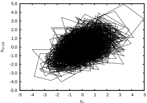
ding space but choosing too large of anmmay cause the vari-ous algorithms to underperform (Kantz and Schreiber, 1997). A practical method for choosing the right embedding dimen-sion, proposed by Kennel et al. (1992), is to find the fraction of false neighbours as a function of the embedding dimen-sion. False neighbours arise when the current dimension is not large enough for the attractor to unfold its true geome-try, leading to crossing of trajectories due to projection onto a smaller dimension. The method checks the neighbours in progressively higher dimensions until it finds only a negli-gible number of false neighbours in passing from dimension mtom+1. The first time the fraction of false neighbours attains a minimum indicates a suitable value for the embed-ding dimension. For the present data, Fig. 7 plots the frac-tion of false neighbours as a funcfrac-tion of embedding dimen-sion and it can be seen that an optimal choice ofmmust be higher than 13, since form≥13 the fraction of false neigh-bours becomes negligibly small. We have chosenm=14 for the further analysis. It may be noted that, for most of the practical purposes, the important embedding parameter is the productmτ of the embedding dimension and the delay time because mτ is the time span represented by an embedding vector. Only a precise knowledge ofmis required to exploit the determinism of the underlying dynamics with minimal computational effort (Kantz and Schreiber, 1997). The de-lay representation of the denoised detrended time series with m=14 andτ =1 is shown in Fig. 8. The definite structure in the Fig. 8 indicates the deterministic nature of the data.

-5.0 -4.0 -3.0 -2.0 -1.0 0.0 1.0 2.0 3.0 4.0 5.0

-5 -4 -3 -2 -1 0 1 2 3 4 5

yn+14

y_n

Fig. 8. The delay representation of the detrended time series.

various dimension estimates, the easiest to compute from a given time series, and which has also become the standard now, is the correlation dimension introduced by Grassberger and Procaccia (1983). The correlation dimensionD2is de-fined in terms of the correlation integralC(), which is de-fined as the probability that a pair of points chosen randomly on the attractor is separated by a distance less than. On the attractor, the correlation integral is empirically found to scale likeC()∝D2 _{as→0, so that the correlation dimension}

may be estimated as the slope of the curve of lnC()versus ln()given by

D2=lim →0

d lnC()

d ln . (5)

In practical computations involving a single time series and N data points ofm-dimensional delay vectorsyi, the

corre-lation integralC()is approximated by the correlation sum C(, m)given by (Kantz and Schreiber, 1997)

C(, m)= 2

N (N−1) N X

i=1 N X

j=i+1

2(− ky_i−y_jk), (6)

for sufficiently largeN, where2(a)=1 ifa >0,2(a)=0 ifa≤0. The scaling exponent in Eq. (5), when calculated using the correlation sumsC(, m), typically increases with mand saturates to a final value for sufficiently largemwhich is then taken as an estimate forD2. In practice, one computes the local slopes with the following equation:

D2(, m)=d lnC(, m)

d ln (7)

and plots them as a function of for various m; the value corresponding to a plateau in the curves is identified as an approximation to D2. There are, however, some subtleties to be taken care of in the computation of correlation di-mension. While only the spatial closeness of points should be accounted for in Eq. (7), the actual computations may

0 2 4 6 8 10

0.1 1

D2

(

ε

,m)

ε

Fig. 9. The local slopesD₂(, m)for the detrended time series for

mranging from 14 to 16 withτ=1, ω=25 giving a plateau for small values ofand giving an estimate ofD2=3.7967±0.0116.

The convergence of the plateau for higher dimensions is also evident in Fig. 11a indicating evidence of low dimensionality.

be affected by the temporal closeness of points as well. To guard against this, points that are closer in time by less than a Theiler windowω– which is approximately equal to the product of the time delay and the embedding dimension – are excluded while calculating the correlation sum (Theiler, 1986). Hegger et al. (1999) have suggested that the value of ωshould be chosen generously.

Figure 9 plots the local slopesD2(, m)for the DMWS-data with the previous choice of delay and for embedding dimensions ranging from 14 to 16 using 25 as value for Theiler window. The curves exhibit convergence for larger m, an indication of low dimensionality of the attractor, and suggest a value ofD2=3.7967±0.0116. This shows that, while the original system may be affected by a multitude of factors, the eventual behaviour can be characterised by a low-dimensional attractor.

-1.0 -0.9 -0.8 -0.7 -0.6 -0.5 -0.4 -0.3 -0.2

0 5 10 15 20 25 30 35 40

S(

Δ

n)

Δn

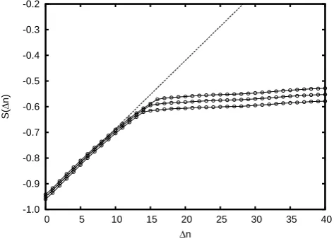
Fig. 10. The curve ofS(1n)for the embedding dimensionsm=

14,15,16 withτ=1, ω=25.The maximum Lyapunov exponentλ

of the detrended time series is the slope of the dashed line 0.0265±

0.0008.

thatkδ(t )| = kδ(0)keλt, and hence λ= lim

t→∞ 1 t ln

kδ(t )k

kδ(0)k. (8)

In practice one computesλby plotting lnδ(t )versust, which should fall nearly on a straight line, the slope of which then gives an estimate ofλ. Lyapunov exponents are invariant un-der smooth transformations of the attractor; hence, they are preserved under delay reconstruction and may be estimated from a time series. There are many algorithms for estimat-ing the maximal Lyapunov exponent from time series, all of which implement the above ideas to delay vectors in the em-bedding space. Most popular among them is the Kantz algo-rithm (Kantz, 1994; Kantz and Schreiber, 1997), which pro-ceeds by computing the sum:

S(1n)=

1 N

N X

n0=1

ln ₁

kU (y_n 0)k

X

yn∈U (yn0)

yn0+1n−yn+1n

(9)

for a pointy_n

0 of the time series in the embedded space and

over a neighbourhoodU (y_n

0)ofyn0 with diameter. If the

plot ofS(1n)against1nis linear over small1nand for a reasonable range of, and all have identical slope for suf-ficiently large values of the embedding dimensionm, then that slope can be taken as an estimate of the maximum Lya-punov exponent (Kantz, 1994; Kantz and Schreiber, 1997). For our time series, Fig. 10 shows curves of S(1n) for m=14,15,16 which increase linearly with1nand then set-tle down. An estimate for the maximum Lyapunov exponent as obtained from the figure isλ=0.0265±0.0008. The com-putations were repeated for various values of the embedding dimension and the diameter of the neighbourhoodU (y_n

0),

all of which gave results identical to the above. The estimated

0 2 4 6 8 10

0.1 1

D2

(

ε

,m)

ε

(b) 0

2 4 6 8 10

0.1 1

D2

(

ε

,m)

ε

(a)

Fig. 11. (a) The local slopesD2(, m)of original time series for the

embedding dimensionsm=1, . . . ,24 withτ=1, ω=25. (b) The same for the phase randomized time series.

positive value of the maximum Lyapunov exponent indicates that the underlying system is chaotic.

A colour noise time series can mimic many characteristics of a chaotic time series. In order to make a distinction be-tween these two, we compared the DMWS time series with its phase randomized time series. The phase randomization of a chaotic signal can destroy its profile, whereas a colour noise time series retains its profile (Pavlos et al., 1992). The phase randomized time series of DMWS data was obtained by representing it by Fourier series and then reconstructing the time series after adding a random phase distribution. We calculated the local slopes of the logarithmD2(, m)of the correlation sum for both the original time series and the phase randomized time series and plotted the values in Fig. 11a and b respectively. These figures clearly show that phase random-ization destroys deterministic profile.

The estimated values of the correlation dimension and the fraction of false nearest neighbours obtained for various em-bedding dimensions show that the underlying dynamics of the fluctuations in the DMWS data is low-dimensional. The positive value of the maximum Lyapunov exponent indicates that the underlying system is chaotic. The comparison of the DMWS data with its phase randomized time series further confirms the chaotic nature of the underlying system.

4 Comparison with surrogate data

-0.20 0.00 0.20 0.40 0.60 0.80 1.00

1 2 3 4 5 6 7 8 9 10

Fraction of False Nearest Neighbours

Embedding Dimension (a)

Mean Mean +- SD Original

0.00 1.00 2.00 3.00 4.00 5.00 6.00 7.00 8.00 9.00 10.00

1 2 3 4 5 6 7 8 9 10

S

Embedding Dimension

(b) S

2

Fig. 12. (a) The mean values of the fraction of false nearest

neigh-bours of the surrogates with standard deviation. (b) Plot of the sig-nificance of differenceSversusm.

section, we must ascertain that the source of the complex be-haviour exhibited by the DMWS-data is not stochastic.

The method of surrogate data (Theiler et al., 1992) is widely used as a tool for discriminating whether the source of random fluctuations in time series data is deterministic or stochastic. It is basically a statistical test to formally reject the hypothesis that the observed data convey a linear noise process. The method proceeds by first formulating a null hy-pothesis, which is usually an assumption that the observed data are random, and then generating an ensemble of time series of random numbers, called surrogate data, which are consistent with the null hypothesis and are otherwise similar to the original data. In other words, these surrogate data are what independent, repeated observations of the process that generated the original data would yield if that process were consistent with the null hypothesis. Then one compares the values of some discriminating statistic, such as correlation dimension, computed from the given data to the distribution of values obtained from the surrogates. If the values differ significantly, then the null hypothesis may be rejected.

0 5 10 15 20 25 30

0.1 1

D2

(

ε

,m)

ε

(a) _{Mean +- SD}Mean

Original

0 5 10 15 20 25 30 35 40 45 50

0.1 1

S

ε

(b) S

2

Fig. 13. (a) The mean values of the local slopes of the surrogates

with standard deviation. (b) Plot of the significance of differenceS

versus. Here the normalised data sets are used, andm=14, τ=1,

andω=25.

-1.0 -0.9 -0.8 -0.7 -0.6 -0.5 -0.4 -0.3 -0.2

0 5 10 15 20 25 30 35 40

S(

Δ

n)

Δn (a)

Mean Mean ± SD Original

0 5 10 15 20 25 30 35

0 5 10 15 20 25 30 35 40

S

Δn

(b) S

2

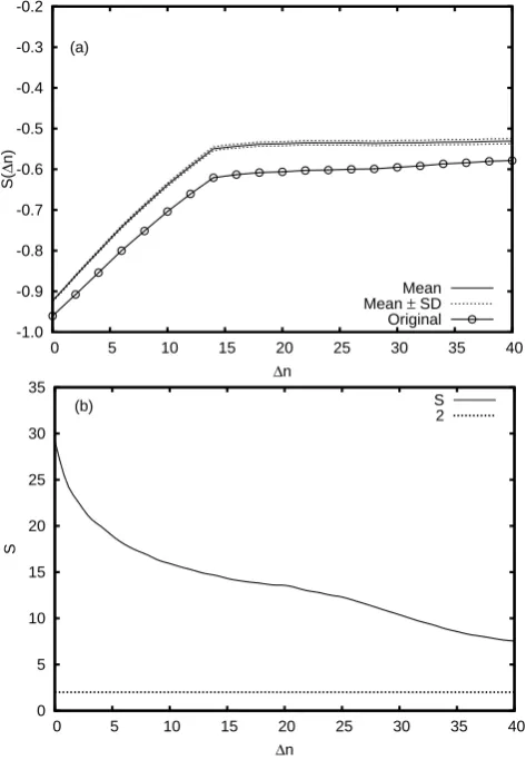
Fig. 14. (a) The mean values ofS(1n)of the surrogates with stan-dard deviation. (b) Plot of the significance of differenceS versus

1n.

Pavlos et al., 1999)

S=µ−µorig

σ (10)

whereµ andσ are the mean and standard deviation of the characteristic computed from the surrogates andµorig is the mean of the characteristic on the original data. It is estimated that we may reject the null hypothesis with 95 % confidence ifS >2, which means that the probability is 95 % or more that the observed time series is not a realisation of a Gaussian stochastic process (Pavlos et al., 1999).

Figure 12a plots the mean values of fraction of false near-est neighbours of all the surrogates and values one standard deviation away from the mean, alongside the values of frac-tion of false nearest neighbours of the DMWS-data. We can observe that the curves of fraction of false nearest neighbours versusmof all the surrogates deviate significantly from the corresponding curve of the original data for a range of the embedding dimensions. As shown in Fig. 12b, the signifi-cance of differenceSfor the fraction of false nearest

neigh-1.040 1.050 1.060 1.070 1.080 1.090 1.100 1.110 1.120

0 5 10 15 20 25 30 35 40 45

Prediction error

The original and surrogates surrogates

original

Fig. 15. The plot of the prediction errors form=14, τ=1 for the surrogates (denoted by circles) and that of the original series (de-noted by filled square), showing the determinism in the time series. The significance of differenceS=4.15.

-0.15 -0.10 -0.05 0.00 0.05 0.10 0.15 0.20 0.25

0 5 10 15 20 25 30 35 40 45

Time reverse asymmetry statistic

The original and surrogates surrogates

original

Fig. 16. The plot of the time reversal asymmetry statistic for delay τ=14 for the surrogates (denoted by circles) and that of the orig-inal series (denoted by filled square), showing the determinism in the time series. The significance of differenceS=2.95.

bours reaches up to 9, and hence the null hypothesis can be safely rejected.

Next we compared the local slopes of the correlation sums. Figure 13a compares the local slopesD2(,14)of the corre-lation sums (Eq. 7), of the DMWS-data with the mean values of the slopes of all the surrogates along with values one stan-dard deviation away from the mean. It is clear that the val-ues of the slopes of the surrogates deviate considerably from those of the original data, especially in the region of smaller . As is clear from Fig. 13b, the significance of difference is large enough to reject the null hypothesis.

1.0 1.1 1.1 1.1 1.1 1.1 1.1 1.1 1.1

5 10 15 20 25 30

Prediction error

Embedding dimension

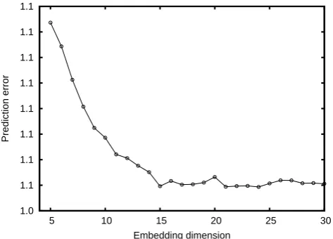
Fig. 17. The plot of the prediction error versus embedding

dimen-sionm.

of the original data plotted for delay τ =1 Theiler win-dowω=25 and embedding dimensionm=14. We observe strong differences between the values ofS(1n) correspond-ing to the original data and the surrogates. The significance of differenceS, shown in Fig. 14b, is larger than 2 for all 1n≤40. Here again, based on the values ofS, we can reject the null hypothesis.

The alignment of the neighbouring segments of trajecto-ries in a flow, which ultimately leads to a definite structure for the attractor if the dynamics is deterministic, can be used as a criterion to distinguish determinism from stochastic dy-namics. A straightforward way to quantify this is the non-linear prediction error which computes the deviations of the values predicted using past data from the actual values in the trajectory. It is reported that the non-linear prediction error is a consistently good tool for discriminating non-linearity (Schreiber and Schmitz, 1997). We calculated the prediction errors by using a locally constant approximation to predict future values (Tong, 1983; Hegger et al., 1999), and the root-mean-square prediction errors of each of the 40 surrogates and the original data were computed. The results are dis-played in Fig. 15 which shows that the prediction errors are significantly lower for the original data than all the surrogates withS=4.15, and hence the null hypothesis can be rejected. The time reversal asymmetry statistic defined by

Trev=h(yn−yn−τ) 3_i

h(yn−yn−τ)2i

(11) is frequently used as a measure of deviations from time re-versibility which is a characteristic of linear systems. Fig-ure 16 showsTrevfor all the surrogates and the original data ,and it is seen that time reversal asymmetry of the original data is larger than that of the surrogates withS=2.95; hence, we can reject the null hypothesis.

To summarise, based on the results of these series of statis-tical tests comparing the DMWS-data with their surrogates,

we can reject the null hypothesis with 95 % confidence level and infer that the DMWS-data do not originate from a linear Gaussian process. This further confirms that the results re-ported in the previous section are not an artefact of a stochas-tic system but of a system that is indeed determinisstochas-tic with a low-dimensional chaotic attractor. Although deterministic, the chaotic nature of the data makes long-term predictions prone to errors, but short-term predictions can be made with fairly good accuracy by carefully chosen methods adapted to the data. The average prediction errors of DMWS-data based on a locally constant approximation are shown in Fig. 17 as function of embedding dimension. As is clear from the fig-ure, the prediction error becomes smaller and stabilised for embedding dimensionm≥14 which, besides being a further justification for our choice ofm=14 in the previous analy-sis, furnishes another piece of evidence for the determinism in the data. However, the locally constant approximation is by no means the most suitable for all types of data, and a proper choice of prediction method requires a careful anal-ysis of the data against the various prediction schemes. This will be addressed in a future work.

5 Conclusions

We have carried out a detailed analysis of the daily mean wind speed measured at Thiruvananthapuram from 2000 to 2010 using tools of non-linear time series analysis. The pur-pose of the study was to examine whether the persistent irreg-ular temporal fluctuations exhibited by the data arose from deterministic or stochastic dynamics of the underlying sys-tem. The analysis reveals that the underlying dynamics of DMWS-data is deterministic, low-dimensional and chaotic. The estimated values of correlation dimension and the frac-tion of false nearest neighbours as a funcfrac-tion of embedding dimension indicate the low dimensionality of the system, and the positive value of the maximum Lyapunov exponent shows that the system is chaotic. The reduction and stabiliza-tion of predicstabiliza-tion errors with increase of embedding dimen-sion is further evidence for determinism. A detailed surrogate data analysis, using a number of measures as discriminating statistic, shows that the characteristics shown by the data are not of a stochastic system exhibiting chaos-like behaviour, and corroborates the deterministic character of the system. The analysis further shows that the chaotic profile does not arise from the pseudo-characteristics of a colour noise time series. While most of the chaotic systems reported in the lit-erature are confined to laboratories, this is a natural system showing chaotic behaviour.

Acknowledgements. The authors are grateful to Manoj Changat,

Topical Editor P. Drobinski thanks two anonymous referees for their help in evaluating this paper.

References

Alligood, K. T., Sauer,T. D., and Yorke, J. A.: Chaos-An introduc-tion to dynamical systems , Springer Verlag, New York, 1997. Bantaa, R. M., Senff, C. J., Alvarez, R. J., Langford, A. O., Parrish,

D. D., Trainer, M. K., Darby, L. S., Hardesty, R. M., Lambeth, B., Neuman, J. A., Angevine, W. M., Nielsen-Gammon, J., Sand-berg, S. P., and White, A. B.: Dependence of daily peak O3 con-centrations near Houston, Texas on environmental factors: Wind speed, temperature, and boundary-layer depth, Atmos. Environ., 45, 162–173, 2011.

Bilgili, M., Sahin, B., and Yasar, A.: Application of artificial neural networks for the wind speed prediction of target station using reference stations data, Renewable Energy, 32, 2350–2360, 2007. Brett, A. C. and Tuller, S. E.: The autocorrelation of hourly wind

speed observations, J. Appl. Met., 30, 823–833, 1991.

Cadenas, E. and Rivera, W.: Wind speed forecasting in the South Coast of Oaxaca, Mexico, Renewable Energy, 32, 2116–2128, 2007.

Celik, A. N.: A statistical analysis of wind power density based on the Weibull and Rayleigh models at the southern region of Turkey, Renewable Energy, 29, 593–604, 2004.

Elliott A. J.: A probabilistic description of the wind over Liverpool Bay with application tooil spill simulations, Estuarine, Coastal and Shelf Science, 61, 569–581, 2004.

Finzi, G., Bonelli, P., and Bacci, G.: A Stochastic Model of Surface Wind Speed for Air Quality Control Purposes, J. Appl. Meteo-rol., 23, 1354–1361, 1984.

Fraser, A. M. and Swinney, H. L.: Independent coordinates fors trange attractors from mutual information, Phys. Rev. A, 33, 1134–1140, 1986.

Gavald´a, J., Massons, J., Camps, J., and D´ıaz, F.: Statistical and spectral analysis of the wind regime in the area of Catalonia, Theor. Appl. Climatol., 46, 143–152, 1992.

George, B., Renuka, G., Satheesh Kumar, K., Anil Kumar, C. P., and Venugopal, C.: Nonlinear time series analysis of the fluctu-ations of the geomagnetic horizontal field, Ann. Geophys., 20, 175–183, doi:10.5194/angeo-20-175-2002, 2002.

Grassberger, P. and Procaccia, I.: Measuring the strangeness of strange attractors, Physica D, 9, 189–208, 1983.

Hegger, R., Kantz, H., and Schreiber, T.: Practical implementation of nonlinear time series methods:The TISEAN package, Chaos, 9, 413–435, 1999.

Hennessey Jr., J. P.: Some aspects of wind power statistics, J. Appl. Meteorol., 16, 119–128, 1977.

Hirata, Y., Suzuki, H., and Aihara, K.: Wind modelling and its pos-sible application to control of wind farms, in: Signal process-ing techniques for knowledge extraction and information fusion, edited by: Mandic, D., Golz, M., and Kuh, A., 23–36, Springer, 2008.

Kamal, L. and Jafri, Y. Z.: Time series models to simulate and fore-cast hourly averaged wind speed in Quetta, Pakistan, Solar En-ergy, 61, 23–32, 1997.

Kantz, H.: A robust method to estimate the maximal Lyapunov ex-ponent of a time series, Phys. Lett. A, 185, 77–87, 1994.

Kantz, H. and Schreiber, T.: Nonlinear Time Series Analysis, Cam-bridge University Press, CamCam-bridge, 1997.

Kavasseri, R. G. and Seetharaman, K.: Day-ahead wind speed fore-casting using f-ARIMA models, Renewable Energy, 34, 1388– 1393, 2009.

Kennel, M. B., Brown, R., and Abarbanel, H. D. I.: Determining embedding dimension for phase-space reconstruction using a ge-ometricalconstruction, Phys. Rev. A, 45, 3403–3411, 1992. Kumar, K. S., George, B., Renuka, G., Kumar, C. V. A.,

and Venugopal, C.: Analysis of the fluctuations of the to-talelectron content (TEC) measured at Goose Bay using the tools of nonlinearmethods, J. Geophys. Res., 109, A02308, doi:10.1029/2002JA009768, 2004.

Lorenz, E. N.: Deterministic nonperiodic flow, J. Atmos. Sci., 20, 130–141, 1963.

Mabel, M. C. and Fernandez, E.: Estimation of Energy Yield From Wind Farms Using Artificial Neural Networks, IEEE Trans on Energy Conversion, 24, 459–464, 2009.

Mart´ın, M., Cremades, L. V., and Santab´arbara, J. M.: Analysis and modelling of time series of surface wind speed and direction, Int. J. Climatol., 19, 197–209, 1999.

Mathew, T., George, S., Sarkar, A., and Basu, S.: Prediction of mean winds at an Indian coastal station using a data-driven tech-nique applied on Weibull Parameters, The International Journal of Ocean and Climate Systems, 2, 45–54, 2011.

Mitschke, F. and D¨ammig, M.: Chaos versus noise in experimental data, in: Complexity and chaos, edited by: Abraham, N. B., Al-bano, A. M., Passamante, A., Rapp, P. E., and Gilmore, R., World Scientific, Singapore, 1993.

Mohandes, M. A., Rehman, S., and Halawani, T. O.: A neural net-works approach for wind speed prediction, Renewable Energy, 13, 345–354, 1998.

Monfared, M., Rastegar, H., and Kojabadi, H. M.: A new strategy for wind speed forecasting using artificial intelligent methods, Renewable Energy, 34, 845–848, 2009.

Ott, E.: Chaos in Dynamical Systems , Cambridge UniversityPress, Cambridge, 1993.

Ott, E., Sauer, T., and Yorke, J. A.: Coping with Chaos, Wiley, New York, 1994.

Packard, N. H., Crutchfield, J. P., Farmer, J. D., and Shaw, R. S.: Geometr y from a time series, Phys. Rev. Lett., 45, 712–716, 1980.

Palmer, T. N.: Extended-range atmospheric prediction and the Lorenz model, B. Am. Meteorol. Soc., 74, 49–65, 1993. Palmer, A. J., Kropfli, R. A., and Fairall, C. W.: Signatures of

de-terministic chaos in radar sea clutter and ocean surface winds, Chaos, 5, 613–616, 1995.

Pavlos, G. P., Kyriakov, G. A., Rigas, A. G., Liatsis, P. I., Trochout-sos, P. C., and Tsonis, A. A.: Evidence for strange attractor struc-tures in space plasmas, Ann. Geophys., 10, 309–322, 1992. Pavlos, G. P., Athanasiu, M. A., Kugiumtzis, D., Hatzigeorgiu, N.,

Rigas, A. G., and Sarris, E. T.: Nonlinear analysis of magneto-spheric data Part I. Geometric characteristics of the AE index time series and comparison with nonlinear surrogate data, Non-lin. Processes Geophys., 6, 51–65, doi:10.5194/npg-6-51-1999, 1999.

Ragwitz, M. and Kantz, H.: Detecting non-linear structure and predicting turbulent gusts in surface wind velocities, Europhys. Lett., 51, 595–601, 2000.

Sauer, T. and Yorke, J. A.: How many delay coordinates do you need?, Int. J. Bifurcation and Chaos, 3, 737–744, 1993. Sauer, T., Yorke, J. A., and Casdagli, M.: Embedology, J. Stat.

Phys., 65, 579–616, 1991.

Schreiber, T: Extremely Simple Nonlinear Noise Reduction Method, Phys. Rev. E, 47, 2401–2404, 1993.

Schreiber, T. and Schmitz, A.: Improved surrogate data for nonlin-earity tests, Phys. Rev. Lett., 77, 635–638, 1996.

Schreiber, T. and Schmitz, A.: On the discrimination power of mea-sures for nonlinearity in a time series, Phys. Rev. E, 55, 5443– 5447, 1997.

Sfetsos, A.: A novel approach for the forecasting of mean hourly wind speed time series, Renewable Energy, 27, 163–174, 2002. Takens, F.: Detecting Strange Attractors in Turbulence, in: Lecture

Notes in Math, vol. 898, Springer, New York, 1981.

Theiler, J.: Spurious dimension from correlation algorithmsapplied to limited time series data, Phys. Rev. A, 34, 2427–2432, 1986. Theiler, J., Eubank, S., Longtin, A., Galdrikian, B., and Farmer, J.

D.: Testing for nonlinearity in time series: the method of surro-gate data, Physica D, 58, 77–94, 1992.

Tong, H.: Threshold Models in Non-Linear Time Series Analysis, in: Lecture Notes in Statistics, vol. 21, Springer, 1983.

Torresa, J. L., Garcia, A., Blasa, M. D., and Franciscob A. D.: Forecast of hourly average wind speed with ARMA models in Navarre (Spain), Solar Energy, 79, 65–77, 2005.