Legendre Polynomials and Functions

Legendre Polynomials and Functions

Reading Problems

Outline

Background and Definitions . . . 2

Definitions . . . 3

Theory . . . 4

Legendre’s Equation, Functions and Polynomials . . . 4

Legendre’s Associated Equation and Functions . . . 13

Assigned Problems . . . 16

Background and Definitions

The ordinary differential equation referred to asLegendre’s differential equation is frequently encountered in physics and engineering. In particular, it occurs when solving Laplace’s equation in spherical coordinates.

Adrien-Marie Legendre (September 18, 1752 - January 10, 1833) began using, what are now referred to as Legendre polynomials in 1784 while studying the attraction of spheroids and ellipsoids. His work was important for geodesy.

1. Legendre’s Equation and Legendre Functions

The second order differential equation given as

(1−x2) d

2_y

dx2 −2x

dy

dx +n(n+ 1) y = 0 n >0, |x|< 1

is known as Legendre’s equation. The general solution to this equation is given as a function of two Legendre functions as follows

y =APn(x) +BQn(x) |x| < 1

where

Pn(x) =

1

2n_n!

dn

dxn(x

2 ₋₁₎n _{Legendre function of the first kind}

Qn(x) =

1

2Pn(x) ln

1 +x

1−x Legendre function of the second kind

2. Legendre’s Associated Differential Equation

Legendre’s associated differential equation is given as

(1−x2)d

2_y

dx2 −2x

dy dx +

n(n+ 1)− m

2

1−x2

If we set m= 0in this equation the differential equation reduces to Legendre’s equation.

The general solution to Legendre’s associated equation is given as

y =A Pm_n(x) +B Qm_n(x)

wherePm_n(x)andQm_n(x)are called the associated Legendre functions of the first and second kind given as

Pm_n(x) = (1−x2)m/2 d

m

dxm Pn(x)

Qm_n(x) = (1−x2)m/2 d

m

Legendre’s Equation and Its Solutions

Legendre’s differential equations is

(1−x2) d

2_y

dx2 −2x

dy

dx +n(n+ 1) y = 0 n >0, |x|< 1

or equivalently

d dx

(1−x2)dy dx

+n(n+ 1) y = 0 n >0, |x|< 1

Solutions of this equation are called Legendre functions of ordern. The general solution can be expressed as

y =APn(x) +BQn(x) |x| < 1

where Pn(x) and Qn(x)are Legendre Functions of the first and second kind of ordern.

If n = 0,1,2,3, . . . the Pn(x) functions are called Legendre Polynomials or order n and

are given by Rodrigue’s formula.

Pn(x) =

1

2n_n!

dn

dxn(x

2₋₁₎n

Legendre functions of the first kind (Pn(x)and second kind (Qn(x) of ordern = 0,1,2,3

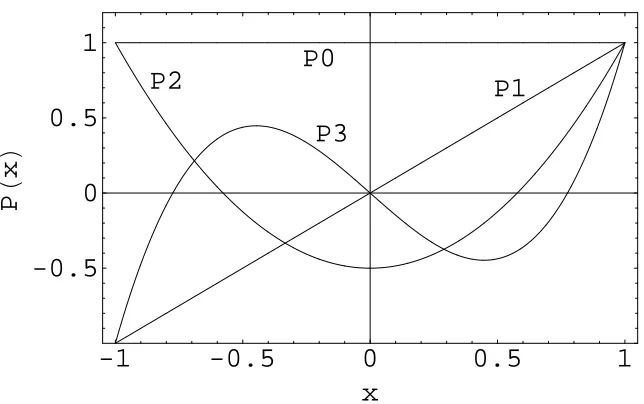
The first several Legendre polynomials are listed below

P0(x) = 1 P3(x) =

1

2(5x

3 _−3x)

P1(x) = x P3(x) =

1

8(35x

4 _−30x2_{+ 3)}

P2(x) =

1

2(3x

2₋

1) P3(x) =

1

8(63x

5 ₋

70x3+ 15x)

The recurrence formula is

Pn+1(x) =

2n+ 1

n+ 1 xPn(x)− n

n+ 1Pn−1(x)

P_n+1(x)−P_n−1(x) = (2n+ 2)Pn(x)

can be used to obtain higher order polynomials. In all cases Pn(1) = 1 and

Pn(−1) = (−1)n

Orthogonality of Legendre Polynomials

The Legendre polynomials Pm(x) and Pn(x) are said to be orthogonal in the interval

−1 ≤ x≤ 1 provided

1

−1

Pm(x) Pn(x) dx= 0 m=n

and as a result we have

1

−1

[Pn(x)]2 dx=

2

-1

-0.5

0

0.5

1

x

-0.5

0

0.5

1

P

x

P1

P0

P2

P3

Figure 5.1: Legendre function of the first kind, Pn(x)

-1

-0.5

0

0.5

1

x

-0.75

-0.5

-0.25

0

0.25

0.5

0.75

1

Q

x

Q0

Q1

Q2

_Q3

Orthogonal Series of Legendre Polynomials

Any functionf(x)which is finite and single-valued in the interval −1 ≤x ≤ 1, and which has a finite number or discontinuities within this interval can be expressed as a series of Legendre polynomials.

We let

f(x) = A0P0(x) +A1P1(x) +A2P2(x) +. . . −1 ≤ x≤ 1

= ∞

n=0

AnPn(x)

Multiplying both sides by Pm(x) dx and integrating with respect to x from x = −1 to

x = 1gives

1

−1

f(x)Pm(x) dx =

∞ n=0 An 1 −1

Pm(x)Pn(x)dx

By means of the orthogonality property of the Legendre polynomials we can write

An =

2n+ 1

2

1

−1

f(x)Pn(x) dx n= 0,1,2,3. . .

SincePn(x)is an even function ofxwhennis even, and an odd function whennis odd, it

follows that if f(x) is an even function ofx the coefficients An will vanish when n is odd;

whereas if f(x) is an odd function ofx, the coefficients An will vanish when nis even.

Thus for and even function f(x) we have

An =

  

0 n is odd

(2n+ 1)

1

0

f(x)Pn(x)dx n is even

whereas for an odd function f(x) we have

An =

  

(2n+ 1)

1

0

f(x)Pn(x)dx n is odd

When x = cosθ the function f(θ)can be written

f(θ) = ∞

n=0

AnPn(cosθ) 0 ≤ θ ≤ π

where

An =

2n+ 1

2

π

0

f(θ)Pn(cosθ) sinθ dθ n= 0,1,2,3. . .

Some Special Results Legendre Polynomials

Integral form

Pn(x) =

1

π

π

0

x+!x2 −_{1 cost}n _dt

Values of Pn(x) atx = 0and x =±1

P2n(0) =

(−1)n_{Γ(n+ 1/2)}

√

πΓ(n+ 1) P2n+1(0) = 0

P_2n(0) = 0 P_2n+1(0) = (−1)

n_{2Γ(n+ 3/2)}

√

πΓ(n+ 1)

Pn(1) = 1 Pn(−1) = (−1)n

P_n(1) = n(n+ 1)

2 P

n(−1) = (−1)

n−1 n(n+ 1)

2

|Pn(x)| ≤ 1

The primes denote differentiation with respect to x therefore

P_n(1) = dPn(x)

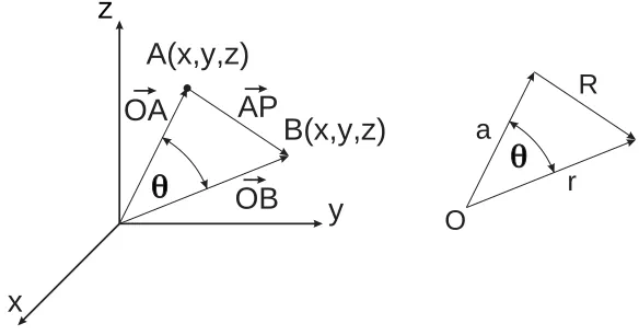
Generating Function for Legendre Polynomials

IfAis a fixed point with coordinates (x1, y1, z1) and P is the variable point(x, y, z) and

the distance AP is denoted byR, we have

R2 = (x−x1)2 + (y−y1)2 + (z−z1)2

From the theory of Newtonian potential we know that the potential at the point P due to a unit mass situated at the point Ais given by

φ= C R

where C is some constant. It can be shown that this function is a solution of Laplace’s equation.

In some circumstances, it is desirable to expand φ in powers of r or r−1 _{where r =} !

x2_+y2 _+z2 _{is the distance from the origin O to the pointP.}

OA

OB

AP

x

y

z

A(x,y,z)

B(x,y,z)

a

R

r

O

Figure 5.3: Generating Function for Legendre Polynomials

a = OA

r = OB

φ = C R =

C

√

Through substitution we can write

φ= C r

1−2xt+t2−1/2

where

t = a

r, x= cosθ

Therefore

φ≡ C

r g(x, t)

We introduce the angleθ between the vectors OA and OP and write

R2 = r2 +a2 −2 cos−1θ

where a =|OA |. If we letr/R = t and x = cosθ, then

g(x, t) = (1−2xt+t2)−1/2

is defined as the generating function for Pn(x). Expanding by the binomial expansion we

have

g(x, t) = ∞

n=0

1

2

n (2xt−t

2₎n

n!

where the symbol (α)n is defined by

(α)n = α(α+ 1)(α+ 2). . .(α+n−1) = Πnk=0−1(α+k)

(α)n is referred to as the Pochammer symbol and(α, n) is the Appel’s symbol.

Thus we have

g(x, t) = ∞ n=0 (1/2)n n! n k=0

n!(2x)n−k_tn−k_(−t2₎k

k!(n−k)!

which can be written as

g(x, t) = (1−2xt+t2)−1/2 = ∞ n=0   n/2 k=0

(−1)k_(2n−2k)!xn−2k

2n_k!(n−_2k)!(n−_k)!

 tn

The coefficient of tn is the Legendre polynomial Pn(x), therefore

g(x, t) = (1−2xt+t2)−1/2 = ∞

n=0

Pn(x)tn |x| ≤ 1, |t| <1

Legendre Functions of the Second Kind

A second and linearly independent solution of Legendre’s equation for n=positive integers are called Legendre functions of the second kind and are defined by

Qn(x) =

1

2Pn(x) ln

1 +x

1−x = Wn−1(x)

where

Wn₋1(x) =

n

m=1

1

mPm−1(x)Pn−m(x)

is a polynomial of the(n−1)degree. The first term ofQn(x)has logarithmic singularities

The first few polynomials are listed below

Q0(x) =

1

2ln

1 +x 1−x Q1(x) = P1(x)Q0(x)−1

Q2(x) = P2(x)Q0(x)−

3

2x

Q3(x) = P3(x)Q0(x)−

5

2x

2 ₊ 2

3

showing the even order functions to be odd in x and conversely.

The higher order polynomials Qn(x) can be obtained by means of recurrence formulas

exactly analogous to those for Pn(x).

Numerous relations involving the Legendre functions can be derived by means of complex variable theory. One such relation is an integral relation of Qn(x)

Qn(x) =

_∞ 0

x+!x2 −_{1 coshθ}−n−1_dθ |_x| _{> 1}

and its generating function

(1−2xt+t2)−1/2cosh−1 √t−x x2 −₁ =

∞

n=0

Qn(x)tn

Some Special Values of Q

(

x

)

Q2n(0) = 0 Q2n+1(0) = (−1)n+1

2·4·6· · · ·2n

1·3·5· · ·(2n−1)

Legendre’s Associated Differential Equation

The differential equation

(1−x2)d

2_y

dx2 −2x

dy dx +

n(n+ 1)− m

2

1−x2

y = 0

is called Legendre’s associated differential equation. If m = 0, it reduces to Legendre’s equation. Solutions of the above equation are called associated Legendre functions. We will restrict our discussion to the important case where m and n are non-negative integers. In this case the general solution can be written

y =A Pm_n(x) +B Qm_n(x)

wherePm_n(x)andQm_n(x)are called the associated Legendre functions of the first and second kind respectively. They are given in terms of ordinary Legendre functions.

Pm_n(x) = (1−x2)m/2 d

m

dxm Pn(x)

Qm_n(x) = (1−x2)m/2 d

m

dxm Qn(x)

The Pm

n(x) functions are bounded within the interval −1 ≤ x ≤ 1 whereas Q m n(x)

functions are unbounded at x =±1.

Special Associated Legendre Functions of the First Kind

P0

n(x) = Pn(x)

Pm

n(x) =

(1−x2₎m/2

2n_n!

dm+n

dxm+n(x

2 ₋₁₎n _{= 0 m > n}

P₁(x) = (1−x2)1/2 P₃(x) = 3 2(5x

2 ₋

1)(1−x2)1/2

P₂(x) = 3x(1−x2₎1/2 _P2

3(x) = 15x(1−x 2₎

P2

2(x) = 3(1−x

2_{) P}3

Other associated Legendre functions can be obtained by the recurrence formulas.

Recurrence Formulas for P

(

x

)

(n+ 1−m)Pm_n+1(x) = (2n+ 1)xP_nm(x)−(n+m)Pm_n−1(x)

Pm_n+2(x) = 2(m+ 1) (1−x2₎1/2 xP

m+1

n −(n−m)(n+m+ 1)P m n(x)

Orthogonality of P

(

x

)

As in the case of Legendre polynomials, the Legendre functions Pm

n(x) are orthogonal in

the interval −1 ≤x ≤ 1

1

−1

Pm_n(x)Pm_k (x) dx= 0 n= k

and also

1

−1

Pm_n(x)2 dx = 2 2n+ 1

(n+m)! (n−m)!

Orthogonality Series of Associated Legendre Functions

Any function f(x) which is finite and single-valued in the interval −1 ≤ x ≤ 1 can be expressed as a series of associated Legendre functions

where the coefficients are determined by means of

Ak =

2k+ 1

2

(k−m)! (k+m)!

1

−1

Assigned Problems

Problem Set for Legendre Functions and Polynomials

1. Obtain the Legendre polynomial P4(x) from Rodrigue’s formula

Pn(x) =

1

2n_n!

dn dxn

(x2 −1)n

2. Obtain the Legendre polynomial P4(x) directly from Legendre’s equation of order 4

by assuming a polynomial of degree 4, i.e.

y =ax4 +bx3 +cx2 +dx+e

3. Obtain the Legendre polynomial P6(x) by application of the recurrence formula

nPn(x) = (2n−1)xPn−1(x)−(n−1)Pn−2(x)

assuming thatP4(x) and P5(x) are known.

4. Obtain the Legendre polynomial P2(x) from Laplace’s integral formula

Pn(x) =

1

π

π

0

(x+!x2 −_{1 cost)}n _dt

5. Find the first three coefficients in the expansion of the function

f(x) =

  

0 −1 ≤x ≤ 0

x 0 ≤x ≤ 1

6. Find the first three coefficients in the expansion of the function

f(θ) =

  

cosθ 0≤ θ ≤π/2

0 π/2 ≤ θ ≤ π

in a series of the form

f(θ) = ∞

n=0

AnPn(cosθ) 0≤ θ ≤ π

7. Obtain the associated Legendre functions P1

2(x), P 2

3(x) and P 3 2(x).

8. Verify that the associated Legendre function P₃2(x)is a solution of Legendre’s associ-ated equation form = 2, n = 3.

9. Verify the result

1

−1

P_nm(x)P_km(x) dx= 0 n= k

for the associated Legendre functions P1

2(x) and P 1 3(x).

10. Verify the result

1

−1

P_nm(x)2 dx = 2 2n+ 1

(n+m)! (n−m)!

for the associated Legendre function P₁1(x).

11. Obtain the Legendre functions of the second kindQ0(x) and Q1(x)by means of

Qn(x) = Pn(x)

_dx

[Pn(x)]2(1−x2)

12. Obtain the functionQ3(x)by means of the appropriate recurrence formula assuming

Selected References

1. Abramowitz, M. and Stegun, I.A., Handbook of Mathematical Functions, Dover, New York, 1965.

2. Arfken, G., “Legendre Functions of the Second Kind,” Mathematical Methods for Physicists, 3rd ed. Orlando, FL: Academic Press, pp. 701-707, 1985.

3. Binney, J. and Tremaine, S., “Associated Legendre Functions,” Appendix 5 in

Galactic Dynamics, Princeton, NJ: Princeton University Press, pp. 654-655, 1987.

4. Snow, C.Hypergeometric and Legendre Functions with Applications to Integral Equa-tions of Potential Theory, Washington, DC: U.S. Government Printing Office, 1952.