Interest Rate Models

Interest Rate Models

Mathematical Theory of Interest Rate Risk Management

presented by

Lane P. Hughston

Professor of Financial Mathematics

Department of Mathematics, King’s College London The Strand, London WC2R 2LS, UK

[email protected] www.mth.kcl.ac.uk

and

Dorje C. Brody

Royal Society University Research Fellow Theory Group, Blackett Laboratory, Imperial College, London SW7 2BZ, UK

Chapter 1

Discount bonds and interest rates. Libor and swap rates. Forward prices and

forward rates. Short rate and forward short rate. Positive interest conditions.

Interest rate derivative structures.

1.1

Discount bonds and interest rates

The formulae involved with interest rate modelling can get complicated. It is important to use an unambiguous scheme of notation that can be carried across a range of different models and at the same time is useful for calculations.

Time 0 denotes the present. Times a, b, c, etc., denote various future times, as do s, t,

u, and so on. Alphabetical order will often be used to suggest chronological order. Occa-sionally, we use an upper case T to draw attention to a particular date (e.g. a termination date).

We use the notation Pab to denote the value at time a of a discount bond maturing at

timeb. At timeb, the bond pays one unit of “currency”. We fix a currency throughout here. In fact, for any class of financial assets we have a corresponding system of discount bonds. Thus, for dollars, Pab denotes the price at time a, in dollars, of a bond that pays one dollar

at the maturity b.

Equally, we can speak of a “sterling” discount bond, or even a “gold” discount bond. In the latter case, Pab could denote the price at time a, in ounces of gold, of a contract delivering

one ounce of gold at timeb.

Occasionally, a comma will be inserted for clarity. ThusPt,x+tdenotes the value of a discount

bond at time t that matures at time x+t.

Associated with any discount bondPab there are various rates that can be quoted.

For example, thesimple interest rate Lab is defined by:

Pab = 1

1 + (b−a)Lab. (1.1)

The continuously compounded rate Rab is defined by:

Pab =e−(b−a)Rab. (1.2)

The unit of time is one calendar year, and these rates are quoted in an “annualised” basis. Inverting these relations we find that the simple rate is given by

Lab = 1

b−a

1

Pab −1

(1.3)

The corresponding expression for the continuously compounded rate is

Rab =− 1

b−alogPab. (1.4)

1.2

Libor and Swap rates

The Libor rate for a given period is usually quoted on a simple annualised basis, so some-times we call Lab the Libor rate associated withPab.

Note that although rates can be quoted in various ways, the discount bond price is unique (it is a price!). That is a good reason for focusing on discount bonds. These are the fundamental “assets” of interest rate theory, and it is their behaviour we are trying to model.

Another very important type of rate frequently quoted in the over-the-counter interest rate markets is the swap rate.

There are various types of swap rates, and various conventions dealing with day counts, and so on. It is best therefore to give a mathematically concise definition that can be adapted easily to various situations.

Let 0 denote the present, t some date in the future, and T₁, T₂, . . . , Tn a series of future

dates beyond t.

For each such series (T₁, T₂, . . . , Tn) there is a unique swap rate st.

This rate is determined by the condition that if the rate of interest st is paid on a unit

principal on each of the datesT₁, T₂, . . . , Tnand if the unit principal is paid at timeTn, then

the present value at time t of this cash flow is unity. More specifically, we have the condition

st(PtT1 +PtT2+· · ·+PtTn) +PtTn = 1. (1.5)

Solving for st we have

st= 1−PtTn

PtT₁ +PtT₂ +· · ·+PtT_n (1.6)

The sum

VtT1...Tn =

n

i=1

PtTi (1.7)

is sometimes called the ‘basis point value’ (bpv) at time t associated with the date system

T₁, T₂,. . ., Tn.

We note that because st can always be expressed as a combination of various discount

bond values, it makes sense to speak of derivative payoffs based on st.

A derivative whose payoff depends on st can thus be viewed as a kind of exotic option

based on the discount bonds.

There are elements of convention involved in how real swap rates are quoted. For exam-ple, if st is paid semi-annually (i.e. T1,T2, etc., are spaced at half-yearly intervals), then 2st

1.3

Forward prices and forward rates

The forward price of a discount bond will be denoted by Ptab.

This is the price contracted at timet for purchase of a discount bond at timea that matures at timeb.

A standard arbitrage argument shows that

Ptab= Ptb

Pta

. (1.8)

The argument runs as follows.

Suppose at time t a ‘careless’ market maker is willing to sell me a b-maturity bond on a forward basis at time a for a priceQtab that isless than Ptab.

I would then purchaseQtab/Ptaa-maturity bonds at timet, and simultaneously shortQtab/Ptb

b-maturity bonds.

At the same time I purchase 1/Pta b-maturity bonds on a forward basis from the dealer.

At time a, the a-maturity bonds mature, leaving me with Qtab/Pta in cash, which I uses

to purchase 1/Pta b-maturity bonds (taking advantage of the forward agreement).

Then at time b, the long investment pays off 1/Pta, whereas I owe Qtab/Ptb on the

ma-turing short position.

Since 1/Pta > Qtab/Ptb, I have made a risk free profit.

A similar argument allows me to arbitrage the dealer if a forward price greater than Ptab is

made.

Thus we see that Ptab =Ptb/Pta is the correct forward price for a discount bond.

The associated forward rates are given by

Ptab = 1

1 + (b−a)Ltab

(1.9)

and

HereLtab and Rtab are the forward rates, quoted at time t, for the period [a, b], on a simple

and on a continuously compounded basis, respectively.

We callLtab the forward Libor rate made at timet for the period [a, b].

It also makes sense to speak of a forward swap rate.

This is the swap rate sta contracted at time t for a swap entered into at time a with the

payment dates b₁, b₂, . . . , bn. Then we have

sta = 1−Ptabn

Ptab₁ +Ptab₂ +· · ·+Ptabn

. (1.11)

Clearly we have stt=st.

1.4

Short rates and forward short rates.

The rate rb = lima→bLab is called theshort rate.

This is the rate of interest, at time a, on a very short period loan (e.g., “overnight”), expressed on an annualised basis.

If we assume, as seems reasonable, that Pab is differentiable in the maturity date, then

a short computation shows that

ra=− ∂Pab

∂b

a=b

. (1.12)

Over the short term, “compounding” is irrelevant, and thus lim

a→bLab = lima→bRab. (1.13)

The forward short rate fta is the rate of interest contracted at time tfor a very short period

loan at some later timea.

For example, I might agree today to loan you $1,000,000 for one day, one year from now, at a rate of interest of 6% annualised. Then we would have f₀₁ = 0.06 (a= 0, b= 1).

The forward short rate is also called the “instantaneous forward rate” (for example, in Heath, Jarrow & Morton 1992).

We note that the forward short rate is by definition given by the limit

Thus we have

fta =− ∂Ptab

∂b

a=b

=−∂lnPta

∂a . (1.15)

The latter relation is often effectively adopted as a definition forfta in the literature, but it

is important to see that it is not really a definition: it derives from an underlying economic relation.

The significance of the relation

fta =−∂lnPta

∂a (1.16)

is that it is invertible:

PtT = exp

−

T

t

ftudu

. (1.17)

Thus, at any fixed time t, knowledge of the discount functionPtT at that time, for maturity

T, is equivalent to knowledge of the system of forward short rates ftu determined (i.e.

con-tractable) at that time over the interval u∈[0, T].

Note, incidentally, that (1.17) incorporates the maturity condition PT T = 1.

1.5

Positive interest conditions

For many applications we want to build in an interest rate positivity condition.

This is not automatic in the HJM framework, but later when we examine the Flesaker-Hughston framework and its extensions we will see how this feature can be incorporated. For positive interest we require the following two conditions valid for all 0≤a≤b <∞:

0< Pab ≤1, (1.18)

∂Pab

∂b <0. (1.19)

There are various ways of ensuring these conditions are satisfied. For many models they are not. Whether or not this is a material issue depends on the circumstances.

positive. This is because if someone offers to loan you money at a negative rate of interest, then you can immediately take advantage of them and effect an arbitrage.

The positive interest conditions are sufficient to ensure that all the commonly encountered rates are positive: Libor rates, swap rates, forward Libor and swap rates, short rate, and forward short rate.

1.6

Interest rate derivative structures

Let us now turn to the consideration of interest-rate related contingent claims. First, we need to ask what is meant by an “interest rate derivative”.

One general mathematical way of defining a European-style interest rate derivative is to say that the payout at timeT is any random variable HT that is FT-measurable, where (Ft)

is the natural filtration of the multi-dimensional Brownian motion driving the discount-bond system.

In practice, the payout of an interest rate derivative is specified in terms of one or more well-defined rates associated with the given contract period.

Equivalently, we let HT be specified as a function of the values of one or more discount

bonds during the interval [0, T]. The maturities of these discount bonds may or may not lie in that interval.

For example, the payout

(a) HT = max (PT b−K,0) (1.20)

defines a call option on a discount bond (b > T). The payout

(b) HT =Xmax (LT b−R,0) (1.21)

defines a simplecaplet on the Libor rateLT b, where Ris the cap rate, and X is the notional

paid per interest rate point (e.g., $1,000,000 per interest rate point above R).

Normally, a caplet is paid “in arrears”, meaning the rate is set at some earlier time a, and paid at T, so in that case, the payout is

for the rate LaT set earlier at timea.

However, since LaT is known at time a, we can regard the normal caplet as a derivative

that pays the discounted value Ha =PaTHT at the earlier time a, where HT is the payout

defined in (c).

By definition, we have

PaT = 1

1 + (T −a)LaT. (1.23)

It follows, as we noted earlier, that

LaT = 1

T −a

1

PaT −1

. (1.24)

Therefore, the effective payoutHa at time a is given by the following calculation:

Ha=PaTHT

=XPaT max (LaT −R,0)

=XPaT max

1

T −a

1

PaT −1

−R,0

=Xmax

1

T −a(1−PaT)−RPaT,0

= X

T −amax (1−PaT −(T −a)RPaT,0)

= X

T −a[1 +R(T −a)] max

1

1 +R(T −a) −PaT,0

=Nmax (K −PaT,0). (1.25)

Here the strike K is given by

K = 1

1 +R(T −a) (1.26)

and the notional N is

N = X[1 +R(T −a)]

T −a . (1.27)

There are many subtle ways of transforming one type of interest rate derivative structure into another with the same effective payoff.

This is important both in the marketing and the risk management of such products.

As another example, suppose we consider the case of a swaption, the option to enter into a swap at time t for the dates (T₁, T₂,· · ·, Tn) at a fixed “strike” swap-rate R.

Assuming that the option is to pay the fixed rate R, then the payoff Ht at timet is

Ht=VtT₁...TnMax(st−R,0). (1.28) HereVtT1...Tn =

n

i=1PtTi is the bpv at timet for the coupon dates (T1, T2,· · · , Tn).

Clearly, the option is exercised iff the “actual” swap rate st observed at time t is greater

than R.

Thus an alternative way of writing the swaption payout Ht is:

Ht =

1−PtTn−R

n

i=1

PtTn +

. (1.29)

It should be evident that an alternative interpretation of a swaption is to regard it as an option at time t to acquire (A) a portfolio consisting of a unit of cash and a short position in a Tn-maturity bond, in exchange for (B) a portfolio consisting of R units each of the

Ti-maturity bonds for i= 1,2, . . . , n.

This is the economic interpretation of a swaption in terms of the exchange of actual as-sets.

Chapter 2

Dynamical equations for a non-dividend-paying asset. Money market account

and risk premium process. Martingales, supermartingales and

submartin-gales. Martingale relations for a single asset. Transformation to the risk

neutral measure. No-arbitrage relation for derivatives. Derivative pricing.

Girsanov transformation.

2.1

Dynamical equations for a non-dividend-paying

as-set

For a single asset with limited liability and price process St, the stochastic equation for the

dynamics of St is:

dSt

St =µtdt+σtdWt. (2.1)

This equation is defined on a probability space Π = (Ω,F, P) with filtration (Ft), with

respect to which Wt is a standard Brownian motion.

We assume that µt (drift) and σt (volatility) are adapted to the filtration (Ft).

Initially, we consider the simple situation where (Ft) is generated by Wt. Later, when

other basic assets are brought into play, we let the filtration (Ft) be larger.

We can think of Π as representing the economy, and (Ft) as representing the market in-formation flow up to time t.

For many purposes we can, without serious loss of generality, assume that µt and σt are bounded.

exist, and the relevant martingale conditionis satisfied when this is needed. In practice this condition can often be relaxed in various ways.

If µand σ are constant the solution ofSt is:

St=S0exp µt+σWt−1₂σ2t. (2.2)

This is called the geometric Brownian motion model for St.

The geometric Brownian motion model was introduced by Paul Samuelson, and was used by Fisher Black and Myron Scholes as an assumption in the derivation of their celebrated option pricing formula.

More generally, for path dependent µt and σt, which for simplicity we may here assume

to be adapted and bounded, we have the following solution for the asset price in terms of µt

and σt:

St=S0exp t

0

µsds+

t

0

σsdWs− 1₂

t

0

σ_s2ds

. (2.3)

We regard µt and σt as being specified exogenously.

We can use Ito’s lemma to verify that the stochastic equation is satisfied. First, we note that

dlogSt= dSt

St −

1 2

(dSt)2

S_t2 . (2.4)

Thus squaring each side we have:

(dlogSt)2 =

(dSt)2

S_t2 . (2.5)

So putting these two equations together we get:

dSt

St =dlogSt+

1

2(dlogSt)2 (2.6)

But taking the logarithm of (2.3) we have:

logSt= logS0+ t

0

µsds+

t

0

σsdWs− 1₂

t

0

σ_s2ds. (2.7) So by taking the stochastic differential we obtain

Thus by squaring and only keeping the (dWt)2 =dt term we also have:

(dlogSt)2 =σt2dt. (2.9)

It follows immediately that

dSt

St

=µtdt+σtdWt. (2.10)

2.2

Money market account and risk premium process

To proceed further, we introduce a ‘risk-free’ asset, the money-market account, with price process Bt, satisfying

dBt

Bt

=rtdt, (2.11)

Here rt is the short-term interest rate, which we also assume to be adapted to the market

filtration (Ft).

The solution for the money market account process Bt is

Bt=B0exp t

0

rsds

. (2.12)

Now we introduce the market risk premium process λt, defined for a non-dividend paying

asset by

µt =rt+λtσt. (2.13)

The processλt measures, instantaneously, theextra rate of return offered by the asset, above

the risk-free rate rt, per unit of volatility σt.

Note that in the case of a non-dividend paying asset, and in the absence of risk, the rate of return would be rt.

In the case of a dividend paying asset, the process forµt is given by

µt=rt−δt+λtσt, (2.14)

where δt is the dividend rate.

In the case of a single asset the drift condition (2.13) merely defines λt.

2.3

Martingales, supermartingales and submartingales

Now we derive an important relation that ties together the values of an asset at two different times.

One of the central concepts in the modern theory of finance is the idea of amartingale. The point of the martingale concept is that it gives a mathematical embodiment to the notion of a fair game of chance.

It also helps to clarify in mathematical terms what we mean by aforecast.

In what follows we also need to know about the related concepts of supermartingale, and submartingale.

The concept of supermartingale, in particular, plays a special role in interest rate theory. A stochastic processM is an (Ft)-martingale if

(a) E[|Mt|]<∞, for all t≥0, (2.15)

(b) Ms=E[Mt| Fs], for all s < t. (2.16)

Part (b) of this definition expresses the idea that the expected value of the process at time

t, given information up to time s, is equal to the value of the process at time s.

When there is no ambiguity we sometimes write Et[X] = E[X|Ft] for conditional

expec-tation with respect to the sigma-algebra Ft.

We can modify the definition above to account for martingales defined only for t ∈[0, T∗], where T∗ >0 is a fixed time horizon.

A standard Brownian motion Wt is a martingale. So are, for example, the processes given

by

Mt = 1

2(W 2

t −t), (2.17)

Mt = 1

6(W 3

t −3tWt) (2.18)

1 ₄

Another example is given by

Mt= exp σWt− 1₂σ2t, (2.20)

where σ is a constant.

To see that the process 1₂(W_t2 −t) is a martingale, we observe that

Es[Wt2−t] = Es[(Ws+ (Wt−Ws))2−t]

= Es[Ws2] +Es[(Wt−Ws)2]−t

= W_s2−s. (2.21)

More generally, let us define the polynomial Hn(x, y) by the generating function

exp ξx− 1₂ξ2y= ∞

n=0

ξnHn(x, y). (2.22)

Then for each value ofn, the processHn(Wt, t) is a martingale, and the polynomial examples

mentioned above arise as the first few values of n. The polynomials Hn(x, y) are given by

Hn(x, y) = 1₂yn/2hn(x/

2y), (2.23)

where hn(u) are the standard Hermite polynomials.

Martingales also arise as certain classes of stochastic integrals. For example, if σt is Ft-adapted and bounded, then

Mt =M0+ t

0

σsdWs (2.24)

is a martingale. So is:

Mt=M0exp t

0

σsdWs− 1₂

t

0

σ_s2ds

. (2.25)

A process Xt is an (Ft)-supermartingale if

(c) E|Xt| <∞, for all t≥0, (2.26)

Similarly, a process Xt is an (Ft)-submartingale if

(e) E|Xt| <∞, for all t≥0, (2.28)

(f) Xs ≤E[Xt | Fs], for all s < t. (2.29)

A process is a martingale iff it is both a supermartingale and a submartingale. If Xt is a

supermartingale, then −Xt is a submartingale.

Another important way of generating martingales is by taking conditional expectations. Thus if Z is a random variable such that E[|Z|]<∞, then

Mt=Et[Z] (2.30)

defines a martingale by virtue of the “tower property” of conditional expectationEsEt=Es

for s < t.

2.4

Martingale relations for a single asset

Returning to the case of a single asset, let us introduce the relationship µt= rt+λtσt into

the formula forSt. We then have

dSt

St =rtdt+σt(dWt+λtdt). (2.31)

Equivalently, St is given by

St=S0exp t

0

rsds

exp

t

0

σs(dWs+λsds)− 1₂

t

0

σ2ds

. (2.32)

It follows that

St

Bt

=S₀exp t

0

σs(dWs+λsds)− 1₂

t

0

σ2ds

. (2.33)

Now suppose that we define the process Λt by

Λt = exp

−

t

0

λsdWs−1₂

t

0

λ2_sds

. (2.34)

We call Λt the risk adjustment density or risk premium density martingale. It follows from

Itˆo’s lemma that

Equivalently, by integration of this relation, incorporating the initial condition, we have:

Λt= 1−

t

0

ΛsλsdWs. (2.36)

Thus, assuming λt is bounded, we have the martingale relation

Λs=EsΛt, for all s≤t, where EsΛt:=E[Λt| Fs]. (2.37)

Now we show the following important result: ΛtSt

Bt is a martingale. (2.38)

Indeed, a simple computation shows by completing the squares that: ΛtSt

Bt = exp

t

0

(σs−λs)dWs− 1₂

t

0

(σs−λs)2ds

, (2.39)

and the desired property follows since σt is bounded. The martingale property for ΛtSt/Bt

can be written

ΛsSs

Bs =Es

ΛtSt

Bt

, s < t. (2.40)

This is the formula that links past and future values of St, and thus can be thought of as a forecasting relation.

2.5

Transformation to the risk neutral measure

For any random variable Xt measurable with respect to the sigma-algebra Ft, we define a new probability measure Pλ with expectation

Eλ

s[Xt] = Es[ΛtXt]

Λs . (2.41)

This formula explains why we call Λt a “density”.

The new probability measure (i.e. new rule for taking expectations) obtained in this way is called the risk-neutral measure.

This terminology is reserved for the measure obtained by use of the density Λt associated

Under the risk-neutral measure, we have

Ss

Bs =E λ s

St

Bt

, s < t. (2.42)

That is, the discounted asset price is a martingale (where the discounting is taken with re-spect to the money market account).

Another way of putting this is that in the risk neutral measure the value of the asset is a martingale when expressed in units ofBt, i.e., when we use Bt as a numeraire.

As we shall see, there are other measures associated with other choices of numeraire.

2.6

No-arbitrage relation for derivatives

Suppose that there is a derivative associated with St and its price process is Ht.

We assume that Ht is adapted to the filtration (Ft) like St, and in particular that Ht is

fully characterised by an FT-measurable terminal value HT, i.e. its payoff.

This means intuitively that HT can depend in a very general way on the behaviour of

Wt (and hence St) over the interval [0, T].

Of course, HT might be relatively simple, like a call option HT = max (ST −K,0) or a

short position in a forward contract HT =K−ST.

But it might be path-dependent, like a knock-out option, or an Asian option, or an American option (exercisable at some random time τ ≤ T, with the proceeds future valued and paid at timeT).

For the price dynamics of Ht let us write

dHt

Ht =µ H

t dt+σtHdWt. (2.43)

Then a well-known hedging argument can be used to establish that

µH_t −rt

σ_tH =

µt−rt

σt . (2.44)

We form at time t the portfolio with value Ht − ∆tSt where ∆t is the number of asset

units shorted.

We examine the dynamics of the portfolio over the next small interval of time. The change in the value of the portfolio is given bydHt−∆tdSt.

Then if

∆t= Htσ H t

Stσt

, (2.45)

the “risks” (i.e. the coefficients of dWt) cancel, and the portfolio offers an instantaneously definite rate of return given by

HtµHt −∆tStµt

Ht−∆tSt . (2.46)

We equate this “hedged” rate of return to rt and insert the correct hedge ratio ∆t. Then

the desired no-arbitrage relation

µH_t −rt

σ_tH =

µt−rt

σt . (2.47)

immediately pops out.

This relation is general, and is applicable in a fully path-dependent context.

2.7

Derivative pricing

We have assumed that (a) both the derivative and the asset price are adapted to the same Brownian motion filtration, (b) there are no dividends, (c) there are no transaction costs, (d) there are no constraints (e.g. limits) on the hedge position, and (e) the hedge portfolio can be adjusted continuously.

Note that if we further assume Ht = H(St, t) for some function H(S, t) of two variables,

then the relation above becomes a PDE (the Black-Scholes equation) if µt, σt, rt and λt are

all likewise expressible as such functions.

This leads us down the “classical” path of derivative pricing, which can be highly effec-tive when the assumptions indicated apply.

(b) the asset price dynamics are path dependent.

The implication of the no-arbitrage condition (i.e. the general hedging argument) is thatthe derivative price and the underlying asset both have the same risk premiumλt.

As a consequence, defining Λt as before, it follows that ΛtHt/Bt is a martingale:

ΛsHs

Bs =Es

ΛtHt

Bt

. (2.48)

Equivalently, we have

Hs

Bs =E λ s Ht Bt , (2.49)

where Eλ denotes expectation in the risk neutral measure. In particular, we have

H₀ =E

ΛTHT

BT

. (2.50)

Equivalently:

H₀ =Eλ

HT

BT

. (2.51)

This is the risk-neutral valuation formula which says in words that the present value of a derivative is equal to the risk-neutral expectation of its terminal payoff.

For example, if µ, r and σ are constant, and if HT is a simple call option payoff on ST,

then this reduces to the Black-Scholes formula:

H₀ =S₀N

ln S₀erT/K+1₂σ2T σ√T

−e−rTK N

ln S₀erT/K−1₂σ2T σ√T

(2.52)

where

N(x) = √1 2π

x

−∞

e−12ξ2dξ (2.53)

is the standard normal distribution function.

2.8

Girsanov transformation

We note that in the case of both the asset and the derivative, as a consequence of the no-arbitrage condition, the term dWt+λtdt is common to the dynamics:

dSt

St =rtdt+σt(dWt+λtdt) (2.54)

dHt

Ht =rtdt+σ H

t (dWt+λtdt) (2.55)

Now we define a new processW_tλ according to the formula

W_tλ =Wt+

t

0

λsds. (2.56)

It follows that dW_tλ =dWt+λtdt.

The essence of the theorem of Girsanov is that if Wt is a Brownian motion with respect

to P, then W_tλ is a Brownian motion with respect to Pλ. Then we say that W_tλ is a Pλ -Brownian motion. The dynamics of St and Ht can be written

dSt

St =rtdt+σtdW λ

t, (2.57)

dHt

Ht =rtdt+σ H

t dWtλ. (2.58)

In the risk neutral measure, W_tλ is a Brownian motion.

Thus we see that, as a consequence of the Girsanov transformation, the risk premium effec-tively drops out of the dynamics for both the underlying asset as well as the derivative. With respect to the risk neutral measure both St and Ht have a rate of return given by

rt, the rate of return offered on the locally risk-free money-market asset Bt.

A more precise account of Girsanov’s theorem is as follows.

Let (Ω,F, P) be a probability space equipped with a filtration (Ft). Suppose that Wt is

a n-dimensional (Ft)-Brownian motion defined on this probability space.

Letλα_t be a n-dimensional, (Ft)-measurable process satisfying

P

t

0 |

λs|2ds <∞

Under these assumptions, the process Λt given by

Λt = exp

−1

2 t

0 |

λs|2ds−

t

0

λs·dWs

(2.60) is well defined for all t. We can verify that

Λt= 1−

t

0

Λsλs·dWs, (2.61)

A sufficient condition for Λt to be a martingale is the Novikov condition:

E exp 1 2 t 0 |

λs|2ds

<∞, (2.62)

in which case EΛT = 1. This condition is satisfied, in particular, if λt is bounded.

If Λt is a martingale, then, given any fixed timeT >0, we can define a probability measure

QT on (Ω,FT) by

QT(A) = E[ΛT1A], for all A∈ FT. (2.63)

The Girsanov theorem states that, given any fixed time T >0, the process W_t∗ defined by

W_t∗ =Wt+

t

0

λsds, t ∈[0, T] (2.64)

is a n-dimensional Brownian motion on (Ω,FT, QT).

We can, for example, verify thatW_t∗ is normally distributed with respect to the measureQT

by use of the method of characteristic functions.

Given any t∈[0, T], we calculate the characteristic function of the random variable ˜Wt.

EQ_{T e}izW∗

t ₌EP _ΛTeizWt∗ =EP ΛteizWt∗

=EP exp − t 0

λsdWs−1₂

t

0

λ2_sds+izWt+iz

t

0

λsds

=EP exp − t 0

(λs−iz)dWs− 1₂

t

0

(λs−iz)2ds− 1₂z2t

=EP exp − t 0

(λs−iz)dWs− 1₂

t

0

(λs−iz)2ds

exp −1₂z2t

= exp −1₂z2t. (2.65)

Chapter 3

Dynamical equations for multiple assets. Market completeness. Valuation

of derivatives in complete multi-asset market. Hedgeable and unhedgeable

claims in incomplete markets.

3.1

Dynamical equations for multiple assets

We model the economy by a probability space (Ω,F, P) equipped with standard augmented filtration{Ft}generated by a standardn-dimensional Brownian motionWtα,α = 1,2,· · · , n,

over the time interval 0≤t≤T∗, for some terminal dateT∗. For some applications we may wish to take T∗ =∞.

According to the Ito calculus, we have dW_tαdW_tβ = δαβdt, where δαβ is the identity ma-trix. Note that the different components of W_tα are taken to be uncorrelated.

Let us assume we have a system of m non-dividend-paying risky assets with price processes

dS_ti S_ti =µ

i tdt+

n

α=1

σ_tiαdW_tα. (3.1)

Here, S_ti (i= 1,2,· · · , n) represents the price process for asset number i.

The drift process µi_t and the volatility process σ_tiα are assumed to be bounded and pro-gressively measurable with respect to the filtration{Ft}.

Intuitively speaking, the latter condition means that these processes depend on the path of the Brownian motion from 0 up to timet, but otherwise, there is no source of ‘extraneous’ randomness.

For the moment, we shall not fix the relation between the number of assets m and the number of Brownian motions n.

In the case of a complete market, we normally require that m should be greater than or equal to n.

In other words, for a complete market, there should be at least as many genuinely ‘in-dependent’ assets as there are ‘sources of randomness’.

Otherwise, there may be more sources of randomness than there are independent means of hedging away this randomness! That would mean an ‘incomplete’ market.

At time t, the relative magnitude of the price fluctuation of asseti due to Brownian motion number α is given by σ_tiα, which we call the volatility matrix.

The exogenous specification of µi_t and σiα_t determines the asset price processes S_ti, once initial prices have been given, according to the formula

S_ti =S₀iexp t

0

µi_s−1₂σi_s2ds+ t

0

σ_sidWs

. (3.2)

Here we use the compact notation

σi_sdWs = n

α=1

σ_siαdW_sα (3.3)

and

σ_si2 =

α

σiα_s σiα_s . (3.4)

For each fixed value of i, we think of σi_s as a vector volatility process with n components, one for each of the n independent Brownian motion.

3.2

Market completeness

More precisely,σ_tiαis of maximal ranknat timetif, for any nonzero vectorηα = (η1, η2,· · · , ηn) we have

n

α=1

ηασiα_t = 0. (3.5)

If this holds for all ηα = 0, then any fluctuation dW_tα in the Brownian motion results in a nontrivial asset price fluctuation dS_ti.

This is evident from the basic dynamical equations.

Additionally, we will sometimes require to impose a condition on the volatility structure, sufficient to keep it from getting to ‘close’ to degeneracy.

This can be imposed by requiring that the symmetric matrix

ραβ_t =

m

i=1

σ_tiασ_tiβ (3.6)

satisfies the condition that there exists a number such that

ραβ_t > δαβ. (3.7)

In other words

α,β

ραβ_t −δαβ

ηαηβ >0 (3.8)

for any nonvanishing vector ηα. This ensures that the eigenvalues of ραβ_t are bounded from below by .

3.3

Absence of arbitrage in a multi-asset context

Now let us consider the principle of no arbitrage.

This principle implies in the case of an asset that pays no dividend that the drift is of the form

µi_t=rt+ n

α=1

for some progressively measurable vector process λt, independent of the value of i.

This is the market risk premium vector, which has the interpretation of being the extra rate of return, above the interest rate, per unit of volatility in the factorα.

Hence, the no-arbitrage condition tells us that the given family of assets shares a com-mon risk premium process λα_t.

Once we deduce the existence of a market risk premium process, we obtain the following stochastic equation for the asset dynamics:

dS_ti

S_ti =rtdt+

n

α=1

σ_tiα(dW_tα+λα_tdt). (3.10)

We note the important fact that, in a complete market, the risk premium vector isuniquely determined by the given stochastic system.

This follows from the observation that, if (3.9) were satisfied for any other choice of risk premium vector, say,λα_t +η_tα, then the market completeness would imply ηα_t = 0.

In an incomplete market we can then ask whether it is appropriate to regard λα_t as be-ing exogenously specified.

3.4

Valuation of derivatives in complete multi-asset

markets

Consider now the valuation of derivatives in a complete market.

Many aspects of the present analysis have analogues in the case of a single asset, but there are some new twists as well that carry over to interest rate theory.

First, we need to introduce the unit initialised money market account process:

Bt= exp

t

0

rsds

(3.11)

In a complete market with risk premium vector λt, the asset price processes are

S_ti =S₀iexp t

0

rsds+

t

0

σ_si(dWs+λsds)− 1₂

t

0

(σ_si)2ds

As a consequence, we see that the ratios of S_ti toBt (discounted asset prices) are given by

S_ti Bt

=S₀iexp t

0

σi_s(dWs+λsds)− 1₂

t

0

(σ_si)2ds

. (3.13)

The combination dWt+λtdt appearing here suggests that, with a change of measure, the

discounted asset prices will be martingales. To see this, we form the density martingale

Λt = exp

−

t

0

λsdWs−1₂

t

0

λ2_sds

. (3.14)

A short calculation shows that the ratio ΛtSti

Bt =S i 0exp − t 0

(σ_si −λs)dWs− 1₂

t

0

(σ_si −λs)2ds

(3.15)

is a martingale:

ΛsSsi

Bs =Es

ΛtSti

Bt

. (3.16)

This relation has to hold among all the given assets subject to a no arbitrage condition. We may therefore consider the situation where one or more of these assets is a deriva-tive.

Let HT denote the payoff of such a derivative, and let Ht denote the price process for

the derivative at earlier times.

It follows that the value of the derivative is given by:

Ht = Bt

ΛtEt

ΛT

BTHT

. (3.17)

For the present value we then obtain the risk neutral valuation formula:

H₀ =Eλ

HT

BT

. (3.18)

In the dynamics for S_ti we replace rt with rt −δti where δti is the dividend rate, and we

find that

M_ti = ΛtS

i t

Bt +

t

0

ΛuδiuSui

Bu du (3.19)

is a martingale.

Then we can develop pricing formulae where both the assets and the derivatives pay contin-uous dividend.

3.5

Natural numeraire and state-price density

There is an interesting economic interpretation of the basic derivatives pricing formula (3.17). We note that the process Λt is “dimensionless”, whereas Bt is an asset price. Thus, the

ratio Bt/Λt is also an asset price.

Writingξt=Bt/Λt we deduce that the dynamical equation forξt is

dξt

ξt = (rt+λ

2

t)dt+λtdWt. (3.20)

We think of the process ξt as the value process for a special portfolio in the money market

account and the basic risky assets with the value process ξt.

Sometimes the value process ξt is referred to as the “natural numeraire portfolio”.

The present value of any other asset, when valued in units of the numeraire portfolio, acts as an unbiased forecast for the future value of that asset, when expressed in units of the numeraire portfolio at that time. In other words,

S_si ξs =Es

S_ti ξt

. (3.21)

Another useful way of thinking about ξt is to define the related process

Vt= 1

ξt. (3.22)

For any non-dividend-paying asset St we have

St=Et

VT

VtST

. (3.23)

Now suppose that St is a ‘derivative’ that pays one unit of cash at time T.

Then St is the price process PtT of a discount bond with maturity T. Thus:

PtT =Et

VT

Vt

. (3.24)

3.6

Incomplete markets

We now consider more generally the case where the market is not complete.

In practice, it is common to encounter derivatives that cannot be completely hedged. Nevertheless, we may consider a ‘decomposition’ of a given product into a ‘hedgeable’ and ‘unhedgeable’ parts.

If the market in incomplete, then typically then volatility matrix σiα_t is degenerate (i.e. it has one or more zero eigenvalues).

This implies that the risk premium vector λα_t that satisfies the no arbitrage condition (3.9) is not uniquely determined by the specification of the asset price processes.

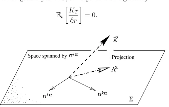
Nevertheless, we may consider the subspace ofRnspanned by the nondegenerate components of the volatility matrixσ_tiα, and construct a decomposition of the form

λα_t =ψ_tα+ϕα_t (3.25)

Here, ψα_t is the vector λα_t with minimum length that satisfies the condition

µi_t=rt+ n

α=1

λα_tσiα_t , (3.26)

whereasϕα_t satisfies

n

α=1

We now define the process ξt by the dynamics

dξt

ξt = rt+ψ

2

t

dt+ψt·dWt (3.28)

This is the unique natural numeraire process corresponding to the hedgeable part of the portfolio.

In other words, ξt is the unique attainable numeraire process.

In a complete market, the derivative price process is given by

Gt=Et

HT

ξT

. (3.29)

However, in an incomplete market, the derivative payout HT contains unhedgeable

compo-nents.

Therefore, we consider the decomposition

HT =JT +KT. (3.30)

Here, JT corresponds to the hedgeable part of the derivative.

This is obtained by taking the conditional expectation Et[HT/ξT], and projecting the

re-sulting martingale into the subspace spanned by the volatility vectorsσ_tiα. Then we let t→T and multiply by ξT to obtain JT.

For the remaining unhedgeable part KT, its expectation is given by

Et

KT

ξT

= 0. (3.31)

Σ

α

λ

σ α

σjα k

Space spanned byσiα _Projection

Chapter 4

Discount bond dynamics.

Interest rate volatility and correlation.

Short

rate and instantaneous forward rate processes. Heath-Jarrow-Morton (HJM)

framework. Valuation and hedging of interest rate derivatives.

4.1

Price processes for discount bonds

Now we turn to the modelling of interest rate dynamics.

The key idea here is to keep the discount bonds in the centre of the stage.

The short rate, forward short rates, Libor rates, forward Libor rates, and swap rates are allsubsidiary processes.

If one focuses on discount bonds, then the theory of interest rates assumes a unified, co-herent shape, and also fits in nicely with the consideration of other asset classes, e.g., foreign currencies, credit-risky bonds, inflation-linked bonds, equities and so on.

As indicated earlier, we write Pab for the value at time a of a discount bond that

ma-tures at time b to deliver one unit of currency. The initial discount function is given by P₀b,

and we have the maturity condition Paa = 1 for all a.

For any given value of b we regard Pab as a stochastic process in the a variable over the

interval 0 ≤ a ≤ b. Thus we have a one-parameter family of assets for which the price processes are given byPab.

We calla the “process index” and b the “maturity index”.

We can infer from context whetherPab refers to “the value at timeaof a bond that matures

We shall assume here that the market is driven by a multi-dimensional family of independent Brownian motions W_tα.

The “factor index” α can be understood (as before) as labelling the basis for a finite di-mensional vector space, or as an “abstract” index representing a Hilbert space element in the infinite dimensional case.

The discount bond dynamics are then given by the stochastic equation

dPab

Pab =µabda+ ΩabdWa (4.1)

Hereµab is the drift process for theb-maturity bond. Ωab is the corresponding vector

volatil-ity process. Both are assumed to be adapted to the filtration (Ft) generated by Wtα.

We require that Ωaa = 0, corresponding to the fact that a maturing bond has zero volatility.

We also make the technically useful assumption that the process Ωab is differentiable in

the maturity index.

More specifically, we assume that there exists a processσas such that

Ωab =−

b

a

σasds, (4.2)

where the minus sign appears as a matter of convention. This relation enforces the constraint Ωaa = 0.

Note that in the term ΩabdWa there is, as indicated earlier, an implied summation over

the suppressed vector indices.

Now we impose the no-arbitrage condition. By the same line of argument as in the multi-asset case this ensures the existence of a risk premium vector λα_a such that the drift µab is

given by

µab =ra+ n

α=1

λα_aΩα_ab. (4.3)

Suppressing vector indices, we write this asµab =ra+λaΩab.

In the discussion on multi-asset dynamics, we regardedraas anexogenously specifiedprocess.

However, in the present consideration, the short rate is given by

ra=− ∂Pab

∂b

a=b

. (4.4)

In fact, we shall show that ra can be effectively eliminated as a fundamental variable, and

an expression for the discount bonds can be derived entirely in terms ofλα_a and Ωα_ab.

Alternatively, we can eliminate Ωα_ab, and an expression for the discount bond can be de-rived in terms of the martingale Λt (which incorporates λαa) and the short rate process rt

(which can be specified arbitrarily). This will be shown later.

These diverse but ultimately equivalent ways of characterising interest rate dynamics are at the root of the variousapparently diverse approaches to modelling that have been developed. Inserting the expression for the drift (4.3) into the dynamics (4.1) of the bond prices, we get

dPab

Pab =rada+ Ωab(dWa+λada). (4.5)

Basic interest rate models usually assume the interest rate market is complete.

This means, in particular, that the process Ωα_ab has to satisfy a nondegeneracy sufficient to ensure that there does not exist at any time a vectorηα such that_αΩα_abηα = 0 for allb > a. In essence, this is equivalent to assuming that any interest rate derivative can be hedged with a suitable self-financing portfolio of discount bonds, together with the money market account. Because the system of discount bonds is infinite, but each individual bond has a finite life, there are various ways in which the completeness condition can be met.

It is important to recognise that completeness is a rather strong assumption, and there-fore may not be realised in practice.

Even if the discount bond market is not complete, there are circumstances in which it is appropriate to regard a definite choice of λa as being specified exogenously.

4.2

Discount bond volatility and correlation

Let us now consider some “local” properties of the discount bond dynamics. The dynamical equations under the assumption of no arbitrage are

dPab

Pab

=rada+ Ωab·(dWa+λada). (4.6)

It follows on account of the Ito relations

dW_tαdW_tβ =δαβdt, dW_tαdt = 0, (dt)2 = 0, (4.7) that

dPab

Pab

2

=|Ωab|2 da. (4.8)

Here |Ωab|2 = αn=1ΩαabΩαab is the squared magnitude of the volatility vector for the bond

with maturity b.

We refer to |Ωab| as thelocal volatility of the b-maturity discount bond.

If we consider bonds of two different maturities, say b and c, then the instantaneous or

local correlation for their price dynamics is given by the process

ρtbc = Ωtb·Ωtc

|Ωtb| |Ωtc|. (4.9)

Clearly we have −1≤ρtbc≤1.

To work out the dynamics of Pab, we need to know the vector processes Ωαtb and λαt.

However, to work out the probability laws for Pab, we only require the scalar combinations

|Ωab|,ρtbc,|λt|, and λt·Ωtb.

4.3

Solution for the discount bond processes

The dynamical equation for the bond price involves the bond volatility, the relative risk, and the short rate.

the relative risk process.

The solution of the bond dynamics can be expressed in the form

Pab =P0bBaexp

a

0

Ωsb(dWs+λsds)− 1₂

a

0 |

Ωsb|2ds

. (4.10)

HereBa is the unit-initialised money market account process, given as usual by

Ba = exp

a

0

rsds

. (4.11)

We observe, on the other hand, that the maturity condition Paa = 1 allows us to solve for

Ba in (4.10).

In particular, if we set a=b, we get:

Ba= (P0a)−1exp

−

a

0

Ωsa(dWs+λsds) + 1₂

a

0 |

Ωsa|2ds

. (4.12)

This shows how the short rate can be expressed in terms of the risk premium vector and the discount bond volatility.

More explicitly, by taking logarithms in (4.12), differentiating with respect to a, and us-ing the relation Ωaa = 0, we get the following formula for ra:

ra=−∂alnP0a+

a

0

Ωsa∂aΩsads−

a

0

∂aΩsa(dWs+λsds). (4.13)

Here∂a denotes differentiation with respect toa. Thus we have solved for ra in terms ofλαa

and Ωα_ab.

In obtaining these expressions, suitable technical conditions are required to be satisfied by the discount bond drift and volatility. We shall return later to address this issue more explicitly.

Inserting formula (4.12) for the money market account into (4.10) for the discount bonds, we then obtain the following general quotient formula for the discount bonds:

Pab =P0ab

exp ₀aΩsb(dWs+λsds)− 1₂₀a|Ωsb|2ds

exp ₀aΩsa(dWs+λsds)− 1₂₀a|Ωsa|2ds

. (4.14)

negoti-In the quotient formula (4.14) note that the numerator and the denominator are essentially similar in structure, except the bin the numerator gets replaced by anais the denominator. The quotient formula is the desired explicit expression for the bond prices in terms of the two exogenous variables, the volatility vector and the relative risk vector, with the elimination of the short rate.

4.4

HJM dynamics for the forward short rate

The forward short rate process is given by

fab =−∂blnPab. (4.15)

From the quotient formula it follows by differentiation that these rates can be expressed as follows:

fab =−∂blnP0b+

a

0

Ωsb∂bΩsbds+

a

0

∂bΩsb(dWs+λsds). (4.16)

Heath, Jarrow & Morton (1992) take a general Itˆo process for the forward short rates as the starting point, and impose appropriate no-arbitrage and market completeness conditions to obtain an expression of the form (4.16).

We writeσab =−∂bΩab for the forward short rate (i.e. instantaneous forward rate) volatility.

It follows that

Ωab =−

b

a

σaudu. (4.17)

This builds in the constraint Ωaa = 0, as we noted earlier.

Then for the forward short rate processes in terms of σab we obtain:

fab =f0b +

a

0

σsb

b

s

σsudu

ds+ a

0

σsb(dWs+λsds). (4.18)

Taking the stochastic differential of this expression on the process index we get

dfab =σab

b

a

σaudu

These are the dynamics of the forward short rate, sometimes called the HJM dynamics. It should be clear that the arbitrage-free dynamics of the discount bond system and the HJM forward short rate dynamics are for most practical purposesentirely equivalent. Given the solution of the stochastic equation forfab, we can use the relation

Pab = exp

−

b

a

faudu

(4.20)

to find the bond price.

The forward short rate processes are important from a conceptual point of view, but it should be noted that practical applications invariably refer back to the bond price process

Pab and the short rate process ra.

4.5

Risk neutral valuation of interest rate derivatives

For the value ofHt at timet of a hedgeable interest rate derivative that paysHT at time T,

we have the forecasting relation ΛtHt

Bt =Et

ΛTHT

BT

. (4.21)

Equivalently, we can write this in the form

Ht =BtEλt

HT

BT

. (4.22)

HereEλ_t denotes conditional expectation in the risk-neutral measure induced by Λt which is

defined by the exponential martingale

Λt= exp

−

t

0

λs·dWs− 1₂

t

0 |

λs|2ds

. (4.23)

One of the important features of interest rate theory is that the discount bonds themselves can be viewed as a species of “derivative”.

As a consequence, if we set HT = 1 in (4.21), we have the following risk-neutral

valua-tion formulafor the discount bond price process:

PtT = Bt

ΛtEt

ΛT

BT

. (4.24)

An expression of this form was derived by Vasicek (1977). In the risk neutral measure this can be written as follows:

PtT = BtEλt

1

BT

= Eλ_t

exp

−

T

t

rsds

. (4.25)

These formulae are often used as a starting point for interest rate modelling.

This is because it is possible to specify λt and rt exogenously, without any a priori

re-lation holding between them.

In particular, it follows from the risk-neutral valuation formula that Ptt = 1, and that

for any choice of the processrt and risk premium density Λt, the ratio

ΛtPtT

Bt (4.26)

is a martingale.

This implies that the bond-price system PtT satisfies the no-arbitrage condition, and thus

qualifies as a bona-fide interest-rate model.

Thus summing up, we see that there are two apparently distinct but nevertheless entirely equivalent ways of “covering” the entire category of interest rate models:

(a) by specifying the relative risk process and vector volatility processes,

(b) by specifying the relative risk density together with the short rate process.

We shall return later to investigate in more detail the problem of how to characterise a general interest rate model, but let us first consider some specific interest rate models.

4.6

Market Models

There are a number of different variations on this approach–too many to attempt to survey here–according to which the forward Libor rates and/or swap rates associated the discount bond system are regarded as the “fundamental” dynamical entities.

In its simplest form, the idea of the market model is as follows. The forward Libor ratesLtab

are defined in a standard way by the relation

Ptab= 1

1 + (b−a)Ltab, (4.27)

where Ptab =Ptb/Pta denotes the forward price made at time t for purchase of a b-maturity

discount bond at time a.

For convenience we introduce a “tenor” parameterδ =b−a, and write Lδ_ta =Ltab.

It is then a straightforward exercise in Ito calculus to work out the dynamics ofLδ_ta, starting from the bond price dynamics given by

dPtT

PtT

=rtdt+ ΩtT(dWt+λtdt). (4.28)

The result is a relation of the following form:

dLδ_ta Lδ_ta =

1 +δLδ_ta

δLδ_ta (Ωt,a−Ωt,a+δ)(dWt+λtdt−Ωt,a+δ). (4.29)

The key observation that follows is that ifωt,a is a prescribed deterministic volatility process

for a given fixed tenor then we can solve the equation 1 +δLδ_ta

δLδ_ta (Ωt,a−Ωt,a+δ) = ωt,a (4.30)

for the bond volatility in terms of the forward Libor rates andωt,a.

This shows that there exists an HJM model with the prescribed deterministic volatility for the given forward Libor rate.

The next step is to change measure so as to eliminate the drift, which can clearly be carried out since now we know the bond volatility process.

It is generally recognised that the market model framework has probably been the single most influential development in interest rate theory in the post-1992 years following the advent of the HJM approach.

Chapter 5

General theory of short rate diffusion models.

Diffusion processes.

The

Feynman-Kac formula. Derivation of the discount bond pricing equation.

5.1

General theory of short rate diffusion models

An interesting and important class of interest rate models can be obtained by assuming:

(a) the short rate is a diffusion process,

(b) the discount bonds depend onrt as a state variable.

Such models are often called “short rate” models.

Many of the most well-known interest rate models fall into this category, including for exam-ple the Vasicek model, the CIR model, the Black-Karazinski model, the Black-Derman-Toy model, the Hull-White model, and the rational lognormal model.

More specifically, we consider a family of discount bond price processes PtT such that

PtT =P(t, rt, T). (5.1)

HereP(t, r, T) is a function of three variables. Thus the short rate acts as a “state variable” for this family of models.

The short rate process rt (t ≥ 0) is assumed to satisfy a stochastic differential equation

of the form

drt=µ(t, rt)dt+σ(t, rt)dWt. (5.2)