Electric field measurements on Cluster: comparing the double-probe and electron drift techniques

SRef-ID: 1432-0576/ag/2006-24-275 © European Geosciences Union 2006

Annales

Geophysicae

Electric field measurements on Cluster: comparing the

double-probe and electron drift techniques

A. I. Eriksson1, M. Andr´e1, B. Klecker2, H. Laakso3, P.-A. Lindqvist4, F. Mozer5, G. Paschmann2,6, A. Pedersen7, J. Quinn8, R. Torbert8, K. Torkar9, and H. Vaith2,8

1_{Swedish Institute of Space Physics, Uppsala, Sweden}

2_{Max-Planck-Institut f¨ur Extraterrestrische Physik, Garching, Germany} 3_{Solar System Division, ESA/ESTEC, Noordwijk, Netherlands} 4_{Alfv´en laboratory, Royal Institute of Technology, Stockholm, Sweden} 5_{Space Sciences Laboratory, University of California, Berkeley, CA, USA} 6_{International Space Science Institute, Bern, Switzerland}

7_{Department of Physics, Oslo University, Norway}

8_{Space Science Center, University of New Hampshire, Durham, NH, USA} 9_{Space Research Institute, Austrian Academy of Sciences, Graz, Austria}

Received: 16 June 2004 – Revised: 29 November 2005 – Accepted: 14 December 2005 – Published: 7 March 2006

Abstract. The four Cluster satellites each carry two instru-ments designed for measuring the electric field: a double-probe instrument (EFW) and an electron drift instrument (EDI). We compare data from the two instruments in a rep-resentative sample of plasma regions. The complementary merits and weaknesses of the two techniques are illustrated. EDI operations are confined to regions of magnetic fields above 30 nT and where wave activity and keV electron fluxes are not too high, while EFW can provide data everywhere, and can go far higher in sampling frequency than EDI. On the other hand, the EDI technique is immune to variations in the low energy plasma, while EFW sometimes detects significant nongeophysical electric fields, particularly in re-gions with drifting plasma, with ion energy (in eV) below the spacecraft potential (in volts). We show that the polar cap is a particularly intricate region for the double-probe tech-nique, where large nongeophysical fields regularly contami-nate EFW measurments of the DC electric field. We present a model explaining this in terms of enhanced cold plasma wake effects appearing when the ion flow energy is higher than the thermal energy but below the spacecraft potential multiplied by the ion charge. We suggest that these condi-tions, which are typical of the polar wind and occur sporadi-cally in other regions containing a significant low energy ion population, cause a large cold plasma wake behind the space-craft, resulting in spurious electric fields in EFW data. This interpretation is supported by an analysis of the direction of the spurious electric field, and by showing that use of active potential control alleviates the situation.

Correspondence to: A. I. Eriksson ([email protected])

Keywords. Magnetospheric physics (Electric fields; Instru-ments and techniques) – Space plasma physics (Spacecraft sheaths, wakes, charging)

1 Introduction

276 A. I. Eriksson et al.: Electric field measurements on Cluster

2 Comparing electric field measurements

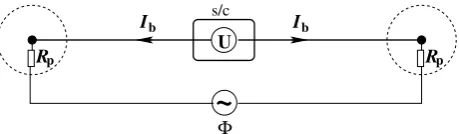
Rp Rp

Ib Ib U Φ

~

Fig. 1.The operational principle of a double probe instrument. Two boom-mounted probes (solid circles) are fed with identical bias

cur-rentsIb. If the resistancesRpover the probe sheaths (dashed

cir-cles) are equal, the voltageUmeasured onboard the spacecraft will

be equal to the potential differenceΦin the plasma between the

probe locations. Unwanted electric field signals can arise either

from a difference inRpbetween the probes, or from an asymmetric

potential structure around the spacecraft and booms adding to the

unperturbedΦin the plasma. Currents close through the spacecraft

sheath (not shown). For a more complete description, see Pedersen et al. (1998).

Fig. 2. The operational principle of the EDI electron drift instru-ment on Cluster, using two gun-detector units (GDU1 and GDU2) emitting two beams of keV electrons and detecting their drift upon

return. For any given magnetic fieldB and drift velocityv, here

assumed to be solely due to an electric fieldE, only one orbit exist

that connects each gun with the opposite detector, enabling a unique

determination ofvand hence ofE. The drawing is not to scale: in

a 100 nT magnetic field, the orbits of the EDI electrons reach 2 km from the spacecraft. For details see Paschmann et al. (2001).

higher than any potentials arising on a well-designed scien-tifc spacecraft (normally less than 50 V). In the weak mag-netic fields typical for Cluster, the emitted electrons also spend most of their time in orbit far away from the spacecraft, further diminishing any influence of the spacecraft-plasma interaction. In addition, the electron drift technique does not depend on spacecraft orientation, while double probe instru-ments at best can have shorter booms along the spin axis and often are confined to measurements in the spin plane. A strength of the EDI technique is that the measurement relies upon simple geometry; thus, when beam tracking is success-ful the absolute measurement is relatively reliable and does not require calibration or offset correction. However, as the electron drift method relies on observing electrons returned to the spacecraft by the ambient magnetic and electric fields, the magnetic field has to be sufficiently strong for the emit-ted beam not to disperse too much for detection. Rapid vari-ations in magnetic or electric field will also complicate the beam tracking, so the method works best in regions where the field variations are less rapid than the tracking bandwidth (∼100 Hz), and the angular stepping rate of the beam. Fur-thermore, sufficiently strong ambient electron fluxes near the beam energy (typically 1 keV) can swamp the beam signal and prevent detection. Table 1 summarizes the performance of the two techniques.

As the strengths and limitations of the two techniques are so different, they complement each other. Each of the four Cluster spacecraft (Escoubet et al., 2001) therefore car-ries one instrument of each type: the double-probe instru-ment EFW (Electric Fields and Waves, Gustafsson et al., 1997; Gustafsson et al., 2001) and the Electron Drift Instru-ment (EDI, Paschmann et al., 1997; Paschmann et al., 2001). Since the start of nominal operations in February 2001, EFW has operated on all four spacecraft essentially all the time. Though EDI operations are restricted to regions with suffi-ciently intense magnetic field, and was operational on Cluster spacecraft four (Tango) only briefly, there is a large amount of simultaneous data from the two instruments available for comparison. In addition, the EDI implementation flying on Cluster is of a design very much improved over previous mis-sions, so there are unprecedented possibilities to compare the performances. Finally, data obtained by both techniques are made widely available to the scientific community through the Cluster Science Data System (Daly, 2002), so there is also an unprecedented need to compare the data in order to provide a background for users of Cluster electric field data. This is the scope of the present study. We cannot exhaust all pitfalls and limitations of either technique in one single paper, but we aim at illustrating the general features, particu-larly pointing out discrepancies arising particuparticu-larly over the polar caps.

It should be noted that in this paper we concentrate on the two Cluster instruments specifically designed for obtain-ing electric field measurements, i.e. EDI and EFW. One may also construct an electric field estimate from the velocity mo-mentvifrom the Cluster ion spectrometers (CIS, R`eme et al., 2001) and the magnetic fieldBfrom the FGM fluxgate

mag-Fig. 1. The operational principle of a double probe instrument. Two

boom-mounted probes (solid circles) are fed with identical bias cur-rentsIb. If the resistancesRpover the probe sheaths (dashed cir-cles) are equal, the voltageU measured on board the spacecraft will be equal to the potential difference8in the plasma between the probe locations. Unwanted electric field signals can arise either from a difference inRpbetween the probes, or from an asymmetric potential structure around the spacecraft and booms adding to the unperturbed8in the plasma. Currents close through the spacecraft sheath (not shown). For a more complete description, see Pedersen et al. (1998).

Each technique has its own merits and weaknesses. Dou-ble probe instruments have relative advantages in terms of conceptual simplicity, regular and essentially unlimited sam-pling frequency, the possibility to measure rapidly vary-ing fields at arbitrarily high amplitudes, and an operational principle independent of the magnetic field. On the other hand, as the measurement principle depends on the electro-static coupling of the probe to the plasma surrounding it, the technique is sensitive to perturbations from the space-craft or the wire booms supporting the probes. Though there are many ways to reduce such perturbations, including de-sign symmetry, biasing of probes and bootstrapping of ad-jacent boom elements, their possible influence always con-stitutes an uncertainty which only comparison to other mea-surements can eliminate. In contrast, electron drift instru-ments are quite insensitive to the details of the spacecraft environment, as the keV energy typical for electrons emit-ted by EDI is much higher than any potentials arising on a well-designed scientifc spacecraft (normally less than 50 V). In the weak magnetic fields typical for Cluster, the emit-ted electrons also spend most of their time in an orbit far away from the spacecraft, further diminishing any influence of the spacecraft-plasma interaction. In addition, the elec-tron drift technique does not depend on spacecraft orienta-tion, while double probe instruments at best can have shorter booms along the spin axis and are often confined to mea-surements in the spin plane. A strength of the EDI technique is that the measurement relies upon simple geometry; thus, when beam tracking is successful the absolute measurement is relatively reliable and does not require calibration or offset correction. However, as the electron drift method relies on observing electrons returned to the spacecraft by the ambient magnetic and electric fields, the magnetic field has to be suf-ficiently strong for the emitted beam not to disperse too much for detection. Rapid variations in the magnetic or electric field will also complicate the beam tracking, so the method works best in regions where the field variations are less rapid than the tracking bandwidth (∼100 Hz), and the angular

step-2

Comparing electric field measurements

Rp Rp

Ib Ib U Φ

~

Fig. 1.The operational principle of a double probe instrument. Two boom-mounted probes (solid circles) are fed with identical bias cur-rentsIb. If the resistancesRpover the probe sheaths (dashed cir-cles) are equal, the voltageUmeasured onboard the spacecraft will be equal to the potential difference Φin the plasma between the probe locations. Unwanted electric field signals can arise either from a difference inRpbetween the probes, or from an asymmetric potential structure around the spacecraft and booms adding to the unperturbedΦin the plasma. Currents close through the spacecraft sheath (not shown). For a more complete description, see Pedersen et al. (1998).

Fig. 2. The operational principle of the EDI electron drift instru-ment on Cluster, using two gun-detector units (GDU1 and GDU2) emitting two beams of keV electrons and detecting their drift upon return. For any given magnetic fieldBand drift velocityv, here assumed to be solely due to an electric fieldE, only one orbit exist that connects each gun with the opposite detector, enabling a unique determination ofvand hence ofE. The drawing is not to scale: in a 100 nT magnetic field, the orbits of the EDI electrons reach 2 km from the spacecraft. For details see Paschmann et al. (2001).

higher than any potentials arising on a well-designed

scien-tifc spacecraft (normally less than 50 V). In the weak

mag-netic fields typical for Cluster, the emitted electrons also

spend most of their time in orbit far away from the spacecraft,

further diminishing any influence of the spacecraft-plasma

interaction. In addition, the electron drift technique does not

depend on spacecraft orientation, while double probe

instru-ments at best can have shorter booms along the spin axis

and often are confined to measurements in the spin plane. A

strength of the EDI technique is that the measurement relies

upon simple geometry; thus, when beam tracking is

success-ful the absolute measurement is relatively reliable and does

not require calibration or offset correction. However, as the

electron drift method relies on observing electrons returned

to the spacecraft by the ambient magnetic and electric fields,

the magnetic field has to be sufficiently strong for the

emit-ted beam not to disperse too much for detection. Rapid

vari-ations in magnetic or electric field will also complicate the

beam tracking, so the method works best in regions where

the field variations are less rapid than the tracking bandwidth

(

∼

100 Hz), and the angular stepping rate of the beam.

Fur-thermore, sufficiently strong ambient electron fluxes near the

beam energy (typically 1 keV) can swamp the beam signal

and prevent detection. Table 1 summarizes the performance

of the two techniques.

As the strengths and limitations of the two techniques

are so different, they complement each other. Each of the

four Cluster spacecraft (Escoubet et al., 2001) therefore

car-ries one instrument of each type: the double-probe

instru-ment EFW (Electric Fields and Waves, Gustafsson et al.,

1997; Gustafsson et al., 2001) and the Electron Drift

Instru-ment (EDI, Paschmann et al., 1997; Paschmann et al., 2001).

Since the start of nominal operations in February 2001, EFW

has operated on all four spacecraft essentially all the time.

Though EDI operations are restricted to regions with

suffi-ciently intense magnetic field, and was operational on Cluster

spacecraft four (Tango) only briefly, there is a large amount

of simultaneous data from the two instruments available for

comparison. In addition, the EDI implementation flying on

Cluster is of a design very much improved over previous

mis-sions, so there are unprecedented possibilities to compare the

performances. Finally, data obtained by both techniques are

made widely available to the scientific community through

the Cluster Science Data System (Daly, 2002), so there is

also an unprecedented need to compare the data in order to

provide a background for users of Cluster electric field data.

This is the scope of the present study. We cannot exhaust

all pitfalls and limitations of either technique in one single

paper, but we aim at illustrating the general features,

particu-larly pointing out discrepancies arising particuparticu-larly over the

polar caps.

It should be noted that in this paper we concentrate on

the two Cluster instruments specifically designed for

obtain-ing electric field measurements, i.e. EDI and EFW. One may

also construct an electric field estimate from the velocity

mo-ment

v

from the Cluster ion spectrometers (CIS, R`eme et al.,

2001) and the magnetic field

B

from the FGM fluxgate

mag-Fig. 2. The operational principle of the EDI electron drift

instru-ment on Cluster, using two gun-detector units (GDU1 and GDU2) emitting two beams of keV electrons and detecting their drift upon return. For any given magnetic fieldB and drift velocityv, here assumed to be solely due to an electric fieldE, only one orbit exists that connects each gun with the opposite detector, enabling a unique determination ofvand hence ofE. The drawing is not to scale: in a 100-nT magnetic field, the orbits of the EDI electrons reach 2 km from the spacecraft. For details, see Paschmann et al. (2001).

ping rate of the beam. Furthermore, sufficiently strong am-bient electron fluxes near the beam energy (typically 1 keV) can swamp the beam signal and prevent detection. Table 1 summarizes the performance of the two techniques.

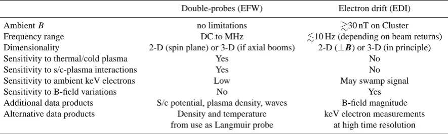
Table 1. Summary of merits and drawbacks of the double-probe and electron drift techniques for magnetospheric electric field

measur-ments. The implementations on Cluster, EFW and EDI, provide 2-D measuremeasur-ments. Extending the EDI technique to three-dimensional measurements will require a significant advance over the current state of the art.

Double-probes (EFW) Electron drift (EDI)

AmbientB no limitations &30 nT on Cluster

Frequency range DC to MHz .10 Hz (depending on beam returns)

Dimensionality 2-D (spin plane) or 3-D (if axial booms) 2-D (⊥B) or 3-D (in principle)

Sensitivity to thermal/cold plasma Yes No

Sensitivity to s/c-plasma interactions Yes No

Sensitivity to ambient keV electrons Low May swamp signal

Sensitivity to B-field variations No Yes

Additional data products S/c potential, plasma density, waves B-field magnitude Alternative data products Density and temperature keV electron measurements

from use as Langmuir probe at high time resolution

It should be noted that in this paper we concentrate on the two Cluster instruments specifically designed for obtain-ing electric field measurements, i.e. EDI and EFW. One may also construct an electric field estimate from the velocity mo-mentvifrom the Cluster ion spectrometers (CIS, R`eme et al., 2001) and the magnetic fieldBfrom the FGM fluxgate mag-netometers (Balogh et al., 2001), assumingE+vi×B=0. We will use this to obtain a “third opinion” on the electric field in cases where EFW and EDI disagree, and we will also in-clude some CIS and FGM data for establishing the geophys-ical context of the data we show, but a complete CIS-EFW comparison, also in regions where there are no EDI data, is outside the scope of the present study, as is any details of measurement errors in the CIS data.

While the Cluster data set for comparison of the two tech-niques surpasses what is available from previous missions, we should note that some comparative studies have been made before. Bauer et al. (1983) and Pedersen et al. (1984) compared data from the two instrument types on the GEOS satellites, finding some effects that we will also see in Clus-ter data. Kletzing et al. (1994) showed data from the F1 (double probes) and F6 (electron drift) instruments on the Freja satellite in the topside ionosphere. Finally, the Geo-tail satellite carries instruments of both kinds, allowing Tsu-ruda et al. (1994) to compare their initial results.

2 EDI–EFW comparison in various plasma regions

2.1 Example 1: Solar wind-magnetosheath-plasma mantle 2.1.1 Geophysical setting

Our first example spans 12 h, from 12:00 to 24:00 UT, on 13 February 2001. The orbit of Cluster during this time in-terval is illustrated in Fig. 3. As can be seen from the model boundaries and field lines in this figure, Cluster should move from the solar wind through the magnetosheath and into the magnetosphere during this time interval. The entry into the

magnetosphere occurs duskward of the southern cusp, so that Cluster at the end of the interval is on field lines reaching the duskside plasma mantle or low-latitude boundary layer.

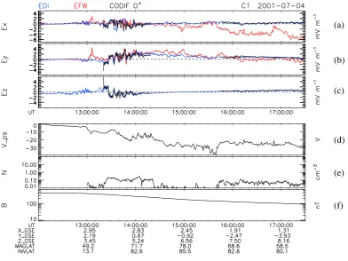
Figure 4 shows 12 h of data from Cluster SC3. The top three panels (a–c) show the electric field measurements that are our real topic here and to which we will return after de-scribing the geophysical setting. The lower three panels (d– f) are auxilliary data for illustration of the plasma environ-ments. As expected from Fig. 3, the spacecraft was in the solar wind at the start of the interval (13 February 2001, 12:00 UT), with weak magnetic field (FGM data, bottom panel f) and a density around 10 cm−3(CIS HIA density mo-ment, panel e). The first bow shock crossing can be seen around 14:40 UT, with an increase in density and magnetic field. The increasing density causes the electrostatic potential of the spacecraft with respect to the surrounding plasma,Vsc, to decrease, as more plasma electrons become available for compensating the emission of photoelectrons. This is seen as a small increase in the EFW probe-to-plasma potential,Vps, which essentially is the negative ofVsc and thus will covary with the density. One may therefore useVpsas a proxy for the plasma density. How to convert fromVpsto plasma density has been reported for Cluster by Pedersen et al. (2001).

The magnetopause is crossed around 20:10 UT, after which the magnetic field (panel (f) of Fig. 4) increases as the spacecraft comes closer to the Earth. In the plasma man-tle, the density as reported from CIS HIA (panel e) and EFW

Vpsdecreases monotonically to reach the limit of the HIA in-strument sensitivity just after 22:00 UT. After this time, the

278 ₄ A. I. Eriksson et al.: Electric field measurements on Cluster_{Comparing electric field measurements}

Fig. 3. Cluster orbit (red) for February 13, 2001, corresponding to the data in Figure 4, viewed from GSE Y (left) and Z (right) directions. Model magnetosheath (light shading) and magnetosphere (dark shading) are shown, as are some magnetic field lines colour coded for magnetic field intensity. Cluster moves inbound, from the solar wind to the magnetosphere. Plot prepared using the Orbit Visualization Tool, http://ovt.irfu.se.

(a)

(b)

(c)

(d)

(e)

(f)

Fig. 4. Comparison of EFW and EDI data from the solar wind through the magnetosheath into the magnetosphere. Panels from top to

bottom: (a)Exin DSI coordinates (almost GSE, see text) in an inertial frame. Red is EFW data based on spin fits from probe pair 12, blue

is EDI, black isxcomponent of−v×Bfrom CIS HIA velocity moment and FGM magnetic field, green is the same for CIS CODIF O+

data. (b,c)EyandEz in same format. (d) EFW probe-to-spacecraft potentialVps ≈ −Vsc. (e) Density moments from CIS: HIA (green,

assuming protons only) and CODIF O+_{(black). (f) FGM magnetic field magnitude.}

4 Comparing electric field measurements

Fig. 3.Cluster orbit (red) for February 13, 2001, corresponding to the data in Figure 4, viewed from GSE Y (left) and Z (right) directions. Model magnetosheath (light shading) and magnetosphere (dark shading) are shown, as are some magnetic field lines colour coded for magnetic field intensity. Cluster moves inbound, from the solar wind to the magnetosphere. Plot prepared using the Orbit Visualization Tool, http://ovt.irfu.se.

(a)

(b)

(c)

(d)

(e)

(f)

Fig. 4. Comparison of EFW and EDI data from the solar wind through the magnetosheath into the magnetosphere. Panels from top to

bottom: (a)Exin DSI coordinates (almost GSE, see text) in an inertial frame. Red is EFW data based on spin fits from probe pair 12, blue

is EDI, black isxcomponent of−v×Bfrom CIS HIA velocity moment and FGM magnetic field, green is the same for CIS CODIF O+

data. (b,c)EyandEz in same format. (d) EFW probe-to-spacecraft potentialVps ≈ −Vsc. (e) Density moments from CIS: HIA (green,

assuming protons only) and CODIF O+_{(black). (f) FGM magnetic field magnitude.}

Fig. 3. Cluster orbit (red) for 13 February 2001, corresponding to the data in Fig. 4, viewed from GSE Y (left) and Z (right) directions.

Model magnetosheath (light shading) and magnetosphere (dark shading) are shown, as are some magnetic field lines colour coded for magnetic field intensity. Cluster moves inbound, from the solar wind to the magnetosphere. Plot prepared using the Orbit Visualization Tool, http://ovt.irfu.se.

4 Comparing electric field measurements

Fig. 3.Cluster orbit (red) for February 13, 2001, corresponding to the data in Figure 4, viewed from GSE Y (left) and Z (right) directions. Model magnetosheath (light shading) and magnetosphere (dark shading) are shown, as are some magnetic field lines colour coded for magnetic field intensity. Cluster moves inbound, from the solar wind to the magnetosphere. Plot prepared using the Orbit Visualization Tool, http://ovt.irfu.se.

(a)

(b)

(c)

(d)

(e)

(f)

Fig. 4. Comparison of EFW and EDI data from the solar wind through the magnetosheath into the magnetosphere. Panels from top to

bottom: (a)Exin DSI coordinates (almost GSE, see text) in an inertial frame. Red is EFW data based on spin fits from probe pair 12, blue

is EDI, black isxcomponent of−v×Bfrom CIS HIA velocity moment and FGM magnetic field, green is the same for CIS CODIF O+

data. (b,c)EyandEzin same format. (d) EFW probe-to-spacecraft potentialVps ≈ −Vsc. (e) Density moments from CIS: HIA (green,

assuming protons only) and CODIF O+_{(black). (f) FGM magnetic field magnitude.}

Fig. 4. Comparison of EFW and EDI data from the solar wind through the magnetosheath into the magnetosphere. Panels from top to

must stay at least below 25 eV after 22:00 UT, and below 10 eV close to midnight. One may also note that this cold plasma shows quite a lot of structure.

The top three panels in Fig. 4 show the electric field mea-surements by EFW (red) and EDI (blue), and the electric field inferred from the FGM magnetic field measurements and the velocity momentsvi from the CIS HIA (green) or CODIF (oxygen ions, black) detectors, assumingE+vi×B=0. The EFW data shown are deduced by fitting a sinusoidal function to the voltage between probes 1 and 2. We have not corrected the EFW data for any well-known effects in double-probe in-struments, like sunward offsets or partial shielding (Pedersen et al., 1998; Maynard, 1998). The impact of such corrections will instead be discussed as data are presented.

To transform CIS velocity moments, we assume that E+vi×B=0. We have chosen to include only EFW mea-surements from the plane in which these are made, i.e. the spin plane, though, in principle, the third component could be derived using magnetometer data andE×B=0 as an as-sumption. All data are therefore given in a reference frame known as despun inverted, or DSI, coordinates, which is a close approximation to GSE but with the Z axis along the spacecraft spin axis. If the spacecraft spin was exactly aligned with the GSE Z axis, the DSI and GSE systems would be identical: for Cluster they differ only by a few de-grees.

It should be noted that all the methods used to deter-mine the electric field signals in this plot, in fact, are two-dimensional, either by being utilized in the spin plane (EFW) or in the plane perpendicular toB (EDI), or by assuming E+vi×B=0 (CIS). Three-dimensional double-probe elec-tric field measurements have been implemented on other spacecraft, for example, on the Polar EFI instrument (Har-vey et al., 1995), using shorter axial booms, and could, in principle, also be implemented by an EDI technique. 2.1.2 Solar wind

In the weak magnetic field in the solar wind, i.e. before 14:40 UT in Fig. 4, EDI cannot provide data, but it is clear that EFW and CIS agree to well within a mV/m. While com-parison of EFW and CIS data is not a prime topic in this paper, we may note in passing that this agreement is typi-cal for spin resolution data in the solar wind, though velocity wakes may at times contaminate the sunward component in higher resolution EFW data, as may be expected in the super-sonically flowing solar wind. A detailed scrutiny will show some tendency, seen most clearly in theEY data in panel (b), for the EFW electric field, to show slightly lower magnitude than expected from CIS velocity. This can be attributed to the effective antenna length being slightly shorter than the phys-ical probe separation, due to the effect of the conductive wire booms on the real electric field. In effect, the booms par-tially short-circuit or shield away the ambient electric field. This effect is well-known (e.g. Mozer, 1973; Pedersen et al., 1998) and results in underestimates of the E-field mag-nitude of some 20% for Cluster EFW in tenuous plasmas. In

panel (a), showing the sunward componentEX, the effect is partially masked by a close-to-constant sunward offset field of 0.5 mV/m. The sunward offset is due to the inevitable photoemission asymmetry between probes on booms point-ing toward and away from the Sun (Pedersen et al., 1998). In the following discussion of other events, we will not further comment on the sunward offset or the partial shielding, but the reader should be aware that these effects always influence double-probe electric field data to some extent.

2.1.3 Magnetosheath

After having entered the magnetosheath, the first time close to 14:40 UT (Fig. 4), EDI data starts appearing intermittently when the magnetic field strength is sufficiently high, the limit typically being around 30 nT. When present, EDI data agrees well with EFW and CIS in this region, despite EDI obviously operating close to and sometimes below its low-B-field limit. An exception is the largeEXjust before 20:00 UT, occurring in a region of enhanced magnetic activity (not shown) which complicates the interpretation of EDI data. CIS shows devi-ations from EDI and EFW, particularly inEX, around 15:00 and 17:00 UT, where the differing values derived from CIS HIA are due to instrumental reasons outside the scope of this paper. For EFW, the magnetosheath usually is a relatively benign region, as the Debye length normally is well below the boom length and the plasma flow is subsonic, thus not creating appreciable wakes.

2.1.4 Plasma mantle

Following the spacecraft into the magnetosphere from 20:10 UT onwards (Fig. 4), we expect the conditions to be-come more suited to the EDI measurement technique as the background magnetic field becomes stronger and less vari-able than in the magnetosheath. This is confirmed by the good agreement we find between EDI and CIS ion data. For the CIS data, the velocity moment after about 21:00 UT must be calculated from the mass-separated data from the CODIF sensor because of the increased relative abundance of oxy-gen. One should note that even though the behaviour of the spacecraft potential shows that the ion detectors only cap-ture a fraction of the ion population, the ion velocity mo-ment should still be reasonably reliably determined as long as there is a sufficient count rate, particularly when using mass-separated data. We thus conclude that EDI works well in this region of the magnetosphere.

2806 A. I. Eriksson et al.: Electric field measurements on ClusterComparing electric field measurements

Fig. 5.Cluster orbit (red) for July 4, 2001, corresponding to the data in Figure 6, viewed from GSE Y (left) and Z (right) directions. Model magnetosheath (light shading) and magnetosphere (dark shading) are shown, as are some magnetic field lines colour coded for magnetic field intensity. The Cluster motion is upward in both projections. Plot prepared using the Orbit Visualization Tool, http://ovt.irfu.se.

(c)

(a)

(b)

(f)

(e)

(d)

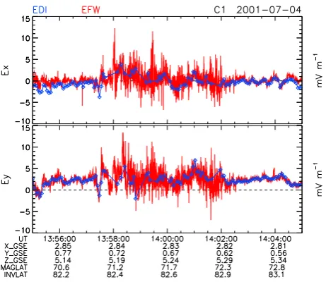
Fig. 6.Comparison of EFW and EDI data from the plasmasphere through the cusp/cleft into the polar cap. Format as in Figure 4.

6 Comparing electric field measurements

Fig. 5.Cluster orbit (red) for July 4, 2001, corresponding to the data in Figure 6, viewed from GSE Y (left) and Z (right) directions. Model magnetosheath (light shading) and magnetosphere (dark shading) are shown, as are some magnetic field lines colour coded for magnetic field intensity. The Cluster motion is upward in both projections. Plot prepared using the Orbit Visualization Tool, http://ovt.irfu.se.

(c)

(a)

(b)

(f)

(e)

(d)

Fig. 6.Comparison of EFW and EDI data from the plasmasphere through the cusp/cleft into the polar cap. Format as in Figure 4.

Fig. 5. Cluster orbit (red) for 4 July 2001, corresponding to the data in Fig. 6, viewed from GSE Y (left) and Z (right) directions. Model

magnetosheath (light shading) and magnetosphere (dark shading) are shown, as are some magnetic field lines colour coded for magnetic field intensity. The Cluster motion is upward in both projections. Plot prepared using the Orbit Visualization Tool, http://ovt.irfu.se.

6 Comparing electric field measurements

Fig. 5.Cluster orbit (red) for July 4, 2001, corresponding to the data in Figure 6, viewed from GSE Y (left) and Z (right) directions. Model magnetosheath (light shading) and magnetosphere (dark shading) are shown, as are some magnetic field lines colour coded for magnetic field intensity. The Cluster motion is upward in both projections. Plot prepared using the Orbit Visualization Tool, http://ovt.irfu.se.

(c) (a)

(b)

(f) (e) (d)

Fig. 6.Comparison of EFW and EDI data from the plasmasphere through the cusp/cleft into the polar cap. Format as in Figure 4.

2.2 Example 2: Plasmasphere-boundary layer-polar cap 2.2.1 Geophysical setting

Our second example is from 4 July 2001, between 12:00 and 17:30 UT. From the orbit plots in Fig. 5, we may ex-pect Cluster to pass from the plasmasphere across boundary layer field lines into the polar cap. Data from Cluster SC1 are presented in Fig. 6, in a format similar to Fig. 4. Panel (d) at first shows Vps values close to zero, corresponding to a plasmaspheric density above 100 cm−3. The plasmapause is crossed in a few minutes just before 12:15 UT, when the den-sity as inferred fromVps drops to∼30 cm−3in a region we may identify as the trough. The density decreases continu-ously to around 15 cm−3at 13:00 UT, where another density drop signals a brief encounter with a part of the plasma sheet extending into the afternoon sector. The increased variations in the electric field, starting around 13:20 UT and continuing until after 14:00 UT, are consistent with the expectation that Cluster here should encounter boundary layer plasmas. Fi-nally, the drop in hot plasma density, as seen by the CIS ion detectors (panel e) around 14:20 UT, signals the start of the open field line region of the polar cap, where the spacecraft remains for the rest of the time interval plotted.

2.2.2 Inner magnetosphere

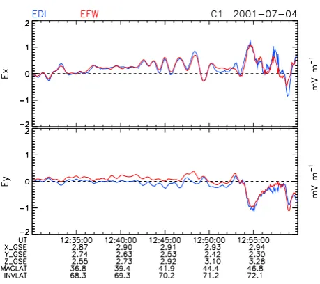
In the plasmasphere and trough regions, i.e. 12:00–13:00 UT in Fig. 6, EFW and EDI are seen in panels (a) and (b) to agree to better than a mV/m in this example, with the largest deviations seen in the plasmasphere (before 12:15 UT). A blowup of part of the trough region is seen in Fig. 7, showing detailed agreement to within 0.1 mV/m in the observation of pulsations, with periods around a minute. The EDI data have been filtered by a boxcar averager, but otherwise no correc-tions or filtering of any kind have been applied to the data.

Such good agreement is commonly found in the trough and subauroral regions, which generally are favourable to EDI and EFW alike. In the plasmasphere, there can some-times be discrepancies due to the formation of plasma wakes (Bauer et al., 1983). However, we find a region of signif-icant difference between EDI and EFW electric field mea-surements between 13:00 and 13:20 UT in Fig. 6. This will be discussed further in Sect. 3.

2.2.3 Plasma sheet and boundary layer

Let us first look at the time interval when Cluster encoun-tered boundary layer field lines, i.e. around 13:20–14:00 UT in Fig. 6, as indicated by the higher level of electric field fluc-tuations. Here, the agreement between EDI and EFW as seen on this time scale again is very good. However, the boundary layer is a very dynamic region, and all dynamics certainly do not show up in this spin-resolution plot. Figure 8 again shows a blowup, with EFW data at full time resolution, which for this case was 25 samples/s. As is to be expected, EDI can-not adequately cover this dynamical situtation, though the data points actually acquired agrees well with EFW. As for

Comparing electric field measurements 7

Fig. 7. Detail of part of the data in Figure 6, showing agreement between EFW (red) and EDI (blue) to the level of a fraction of a mV/m in the inner magnetosphere.

crossed in a few minutes just before 12:15, when the den-sity as inferred fromVps drops to ∼ 30cm−3 in a region we may identify as the trough. The density decreases con-tinuously to around 15 cm−3_{at 13:00, where another density} drop signals a brief encounter with a part of the plasma sheet extending into the afternoon sector. The increased variations in the electric field starting around 13:20 and continuing un-til after 14:00 are consistent with the expectation that Cluster here should encounter boundary layer plasmas. Finally, the drop in hot plasma density as seen by the CIS ion detectors (panel e) around 14:20 signals the start of the open field line region of the polar cap, where the spacecraft remains for the rest of the time interval plotted.

2.2.2 Inner magnetosphere

In the plasmasphere and trough regions, i.e. 12:00 - 13:00 in Figure 6, EFW and EDI are seen in panels (a) and (b) to agree to better than a mV/m in this example, with the largest devi-ations seen in the plasmasphere (before 12:15). A blowup of part of the trough region is seen in Figure 7, showing de-tailed agreement to within 0.1 mV/m in the observation of pulsations with periods around a minute. The EDI data have been filtered by a boxcar averager, but otherwise no correc-tions or filtering of any kind have been applied to the data.

Such good agreement is commonly found in the trough and subauroral regions, which generally are favourable to EDI and EFW alike. In the plasmasphere, there can some-times be discrepancies due to formation of plasma wakes (Bauer et al., 1983). However, we find a region of signif-icant difference between EDI and EFW electric field mea-surements between 13:00 and 13:20 in Figure 6. This will be discussed further in Section 3.

Fig. 8. Detail of part of the data in Figure 6, with EFW (red) and EDI (blue) data at full time resolution in the plasma sheet boundary layer.

2.2.3 Plasma sheet and boundary layer

Let us first look at the time interval when Cluster encoun-tered boundary layer field lines, i.e. around 13:20 – 14:00 in Figure 6 as indicated by the higher level of electric field fluc-tuations. Here, the agreement between EDI and EFW as seen on this timescale again is very good. However, the boundary layer is a very dynamic region, and all dynamics certainly do not show in this spin-resolution plot. Figure 8 again shows a blowup, with EFW data at full time resolution, which for this case was 25 samples/s. As is to be expected, EDI can-not adequately cover this dynamical situtation, though the data points actually acquired agrees well with EFW. As for EFW, the good quality of the data shown here is common not only for boundary layer plasmas but is dominating also in the plasma sheet and auroral zone, and essentially always in the central plasma sheet (not shown). However, spurious fields can sometimes show up in double-probe data, as is illustrated by the large EDI-EFW discrepancy seen in the plasma sheet (Figure 6, 13:00 – 13:20). As was the case in the regions with some EDI-EFW discrepancy in Example 1 (Figure 4), the plasma density indicated by the CIS instrument in this re-gion (below 0.1 cm−3_{) is much lower than what is expected} from the EFWVpsvalue (around 1 cm−3_{), hinting that cold} plasma may be the source of the problem. For the moment, we only note the existence of this kind of problem, which we will discuss in more detail in the following sections.

2.2.4 Polar cap

After leaving the boundary layer field lines around 14:20 UT (Figure 6), the satellite enters the polar cap. The probe-to-spacecraft potentialVpsof panel (d) stays between -20 V and

Fig. 7. Detail of part of the data in Fig. 6, showing agreement

be-tween EFW (red) and EDI (blue) to the level of a fraction of a mV/m in the inner magnetosphere.

EFW, the good quality of the data shown here is common not only for boundary layer plasmas but is also dominating in the plasma sheet and auroral zone, and essentially always in the central plasma sheet (not shown). However, spurious fields can sometimes show up in double-probe data, as is illustrated by the large EDI-EFW discrepancy seen in the plasma sheet (Fig. 6, 13:00–13:20 UT). As was the case in the regions with some EDI-EFW discrepancy in Example 1 (Fig. 4), the plasma density indicated by the CIS instrument in this re-gion (below 0.1 cm−3) is much lower than what is expected from the EFWVpsvalue (around 1 cm−3), hinting that cold plasma may be the source of the problem. For the moment, we only note the existence of this kind of problem, which we will discuss in more detail in the following sections. 2.2.4 Polar cap

After leaving the boundary layer field lines around 14:20 UT (Fig. 6), the satellite enters the polar cap. The probe-to-spacecraft potentialVpsof panel (d) stays between –20 V and –30 V for the remainder of the interval, indicating densities between 1 cm−3and 0.3 cm−3, except for a brief excursion to –40 V (around 0.1 cm−3_{) around 15:35 UT. Comparing to} the CIS CODIF density moment in panel (e), it is clear that the density seen by the ion detector is only a small fraction of the total density, except possibly at the density minimum in-dicated by the EFWVpsat 15:35 UT. In the polar cap region, the plasma component from the CIS data is readily identified as the polar wind, a cold plasma flow known to fill these re-gions in number densities comparable to those indicated by

282 A. I. Eriksson et al.: Electric field measurements on Cluster

Comparing electric field measurements 7

Fig. 7. Detail of part of the data in Figure 6, showing agreement between EFW (red) and EDI (blue) to the level of a fraction of a mV/m in the inner magnetosphere.

crossed in a few minutes just before 12:15, when the den-sity as inferred fromVps drops to∼ 30cm−3_{in a region} we may identify as the trough. The density decreases con-tinuously to around 15 cm−3_{at 13:00, where another density} drop signals a brief encounter with a part of the plasma sheet extending into the afternoon sector. The increased variations in the electric field starting around 13:20 and continuing un-til after 14:00 are consistent with the expectation that Cluster here should encounter boundary layer plasmas. Finally, the drop in hot plasma density as seen by the CIS ion detectors (panel e) around 14:20 signals the start of the open field line region of the polar cap, where the spacecraft remains for the rest of the time interval plotted.

2.2.2 Inner magnetosphere

In the plasmasphere and trough regions, i.e. 12:00 - 13:00 in Figure 6, EFW and EDI are seen in panels (a) and (b) to agree to better than a mV/m in this example, with the largest devi-ations seen in the plasmasphere (before 12:15). A blowup of part of the trough region is seen in Figure 7, showing de-tailed agreement to within 0.1 mV/m in the observation of pulsations with periods around a minute. The EDI data have been filtered by a boxcar averager, but otherwise no correc-tions or filtering of any kind have been applied to the data.

Such good agreement is commonly found in the trough and subauroral regions, which generally are favourable to EDI and EFW alike. In the plasmasphere, there can some-times be discrepancies due to formation of plasma wakes (Bauer et al., 1983). However, we find a region of signif-icant difference between EDI and EFW electric field mea-surements between 13:00 and 13:20 in Figure 6. This will be discussed further in Section 3.

Fig. 8. Detail of part of the data in Figure 6, with EFW (red) and EDI (blue) data at full time resolution in the plasma sheet boundary layer.

2.2.3 Plasma sheet and boundary layer

Let us first look at the time interval when Cluster encoun-tered boundary layer field lines, i.e. around 13:20 – 14:00 in Figure 6 as indicated by the higher level of electric field fluc-tuations. Here, the agreement between EDI and EFW as seen on this timescale again is very good. However, the boundary layer is a very dynamic region, and all dynamics certainly do not show in this spin-resolution plot. Figure 8 again shows a blowup, with EFW data at full time resolution, which for this case was 25 samples/s. As is to be expected, EDI can-not adequately cover this dynamical situtation, though the data points actually acquired agrees well with EFW. As for EFW, the good quality of the data shown here is common not only for boundary layer plasmas but is dominating also in the plasma sheet and auroral zone, and essentially always in the central plasma sheet (not shown). However, spurious fields can sometimes show up in double-probe data, as is illustrated by the large EDI-EFW discrepancy seen in the plasma sheet (Figure 6, 13:00 – 13:20). As was the case in the regions with some EDI-EFW discrepancy in Example 1 (Figure 4), the plasma density indicated by the CIS instrument in this re-gion (below 0.1 cm−3_{) is much lower than what is expected} from the EFWVpsvalue (around 1 cm−3_{), hinting that cold} plasma may be the source of the problem. For the moment, we only note the existence of this kind of problem, which we will discuss in more detail in the following sections.

2.2.4 Polar cap

After leaving the boundary layer field lines around 14:20 UT (Figure 6), the satellite enters the polar cap. The probe-to-spacecraft potentialVpsof panel (d) stays between -20 V and

Fig. 8. Detail of part of the data in Fig. 6, with EFW (red) and

EDI (blue) data at full time resolution in the plasma sheet boundary layer.

that the cold polar wind flow can be seen all the way out to the Polar apogee at 9RE. Since the thermal energy, as well as the bulk flow energy of the ions in the polar wind, are be-low the typically observed spacecraft potential−Vps, we see why this plasma cannot reach the CIS detectors and hence escapes detection.

Differences between the electric field signals from EFW and EDI can be seen in panels (a) and (b) of Fig. 6. Al-though seen in theY component, theXcomponent is most significantly affected. EDI works well in this region, as can be seen by comparing to the E-field estimated from the CIS oxygen velocity moment when this is computable. At times, particularly around 15:30 UT, the data suggests some covari-ance between the EFW-EDI discrepancy andVps. EDI, using keV electrons, should be insensitive to potential variations of the 10 V order, but this is certainly not the case for EFW. The indications thus point to the dominant measurement er-ror originating from EFW rather than from EDI. The event presented here is not an isolated artifact: examples like this are commonly found in EFW-EDI comparisons in the polar cap region, and in preceeding sections in this paper we have seen similar discrepancies for briefer intervals in other re-gions, as well. It is obviously important to understand why: this will be the topic of Sect. 3.

2.3 Summary of events

Summarizing what can be learned from the discussion around Figs. 4 and 6, we conclude that EFW produces good quality electric field data in the solar wind and the magne-tosheath, with some spurious components on the order of a mV/m often appearing in regions with a tenuous cold plasma component in the mantle. EDI produces no data at all in the solar wind and only intermittently in the magnetosheath,

though the electric field estimates are usually good when present, particularly inside the magnetopause. In the plasma-sphere and trough, the two instruments generally agree well, though EFW may sometimes pick up spurious signals, the nature of which we will return to in Sect. 3. This also hap-pens at times in the auroral zone, though this region is usu-ally more problematic for EDI than for EFW, as the strong and rapid electric field variations and the presence of intense auroral electrons may result in an EDI data loss. On the other hand, EDI provides very good data in the polar caps, at least sufficiently close to the Earth to keep the magnetic field above the EDI threshold of about 30 nT, where the EFW data often are severly contaminated or even dominated by spuri-ous electric fields.

3 Polar cap discrepancies

3.1 Spurious field and spacecraft potential

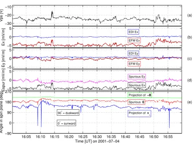
Figure 9 shows a detailed view of 1 h of data from Fig. 6. Panel (a) showsVps, approximately equal to the negative of the spacecraft potential Vsc. During this hour, this quan-tity stays between –20 V and –30 V, corresponding to plasma densities between about 1 cm−3and 0.3 cm−3 (Pedersen et al., 2001), except for an excursion to –15 V, or 1.5 cm−3, at around 800 s. Panels (b) and (c) show the X and Y com-ponents of the electric field from EDI (magenta) and EFW (red/black). The EFW data plotted are spin fits from probe pair 12 (red) and 34 (black). The data from the two probe pairs coincide nearly exactly, so that the black trace is hard to discern.

It can be seen in these panels (b) and (c) of Fig. 9, that EFW and EDI electric field measurements differ by several mV/m during most of this interval. It is interesting to note that this discrepancy is the same regardless of the EFW probe pair used, as the red (P12) and black (P34) curves coincide. If it is the EDI field which is the more accurate representation of the unperturbed electric field in the plasma, the source of the perturbed field seen by EFW must be quite stable. That the field seen by EFW cannot only be the unperturbed elec-tric field in the plasma should be clear from the EDI–CIS agreement shown previously in Fig. 6. A further indication is that the EFW E-field varies with the probe-to-spacecraft potential, Vps. This can be seen more clearly in panel (d), displaying the DSIX(solid) andY (dashed) components of the difference between the instruments,

Espur=EEFW−EEDI. (1)

16:05 16:10 16:15 16:20 16:25 16:30 16:35 16:40 16:45 16:50 16:55 −30

−20 −10

Vps [V]

(a)

16:05 16:10 16:15 16:20 16:25 16:30 16:35 16:40 16:45 16:50 16:55

−5 0 5

(b) EFW Ex

EDI Ex

Ex [mV/m]

16:05 16:10 16:15 16:20 16:25 16:30 16:35 16:40 16:45 16:50 16:55

−5 0 5

(c) EFW Ey

EDI Ey

Ey [mV/m]

16:05 16:10 16:15 16:20 16:25 16:30 16:35 16:40 16:45 16:50 16:55

−5 0 5

(d) Spurious Ex

Spurious Ey

Espur [mV/m]

Cluster SC1 2001−07−04

16:05 16:10 16:15 16:20 16:25 16:30 16:35 16:40 16:45 16:50 16:55

−90 0 90 180 270

(e)

Projection of v_⊥

Projection of −B

Spurious E

0° = sunward 90° = duskward

Angle in spin plane [deg]

Time [UT] on 2001−07−04

Fig. 9.Comparison of EFW and EDI data for an event with a spurious electric field in the EFW data. Panels from top to bottom: (a) EFW

probe-to-spacecraft potentialVps≈ −Vsc. (b)EX(DSI coordinates, see text) in the spacecraft reference frame. Red and black is EFW data

based on spin fits from probe pairs 12 and 34, respectively, blue is EDI. (c)EYin same format. (d) Spurious field in EFW data, assuming

EDI is correct. Black isEX, magenta isEy. (e) Angles of fields projected onto the spin plane, counted from the sun direction, as shown in

Figure 10. Red isEspur=EEFW−EEDI, blue is the projection of EDI perpendicular drift velocity, green is the projection of the negative

of the geomagnetic field (i.e. the direction alongBpointing away from Earth). The spike-like excursions (e.g. around 16:10) originates from

glitches in EDI of no interest here.

in panel (e) of Figure 9. The directions are explained in Fig-ure 10: note that all angles are referring to projections in the spin plane, counted from the solar direction (XDSI≈XGSE) positive towards dusk (YDSI≈YGSE). The green line shows the angle of the projection of−Bonto the spin plane: in the northern hemisphere,−Bis the direction away from Earth along the field lines. The angle of the projection of the EDI flow velocity, vEDI, onto the spin plane is shown in blue. Note that while the full EDI flow velocity vector is necessar-ily perpendicular toBbecause of the EDI operational princi-ple (Section 1), the projections ofvEDIandBonto the spin plane do not need to be perpendicular.

The spin plane direction of the spurious E-field seen by EFW is shown in red. We can see that throughout the in-terval, this angle stays around 180◦_{, superficially suggesting} that the spurious field may be antisunward. However, we may note that the direction ofEspurdepends on the direc-tion of the perpendicular part of the drift velocityv_⊥ deter-mined by EDI, shown in blue. In fact, the spurious field (red) always stays betweenv⊥ (blue) and−B(green). To

deter-mine which direction is the important, we show data from a northern hemisphere dawn-dusk orbit in Figure 11, in the same format as in Figure 9. Jumping directly to panel (e), we see that the spurious field stays between the−Bandv⊥ on this orbit as well, while it does not at all align with the solar direction. This is exactly the direction we expect for the polar wind plasma flow that can be expected in this re-gion of space: EDI should correctly pick up its perpendic-ular componentv⊥ but cannot observe the parallel velocity componentv_k. As the polar wind is an outflow along the geomagnetic field lines, the unobservablev_k should be an-tiparallell to the geomagnetic field, which here points toward Earth. The polar wind velocity vectorv⊥+vkshould thus lie between₋Bandv⊥, precisely as the observed spurious electric field does. This strongly suggests that Espuris re-lated to the plasma flow. In the following section, we will discuss how such a spurious field may arise.

Fig. 9. Comparison of EFW and EDI data for an event with a spurious electric field in the EFW data. Panels from top to bottom: (a) EFW

probe-to-spacecraft potentialVps ≈ −Vsc. (b)EX (DSI coordinates, see text) in the spacecraft reference frame. Red and black represent EFW data based on spin fits from probe pairs 12 and 34, respectively, blue is EDI. (c)EYin same format. (d) Spurious field in EFW data, assuming EDI is correct. Black isEX, magenta isEY. (e) Angles of fields projected onto the spin plane, counted from the Sun direction, as shown in Fig. 10. Red isEspur=EEFW−EEDI, blue is the projection of EDI perpendicular drift velocity, green is the projection of the negative of the geomagnetic field (i.e. the direction alongBpointing away from the Earth). The spike-like excursions (e.g. around 16:10 UT) originate from glitches in EDI, which are of no interest here.

evidence that the problem indeed is with the double-probe method. We thus conclude that the type of EFW-EDI dis-crepancy encountered in the polar cap is due to a spurious field,Espur, adding to the natural field in the EFW data.

3.2 Direction of spurious field

To obtain further information on the spurious field, we will now study its direction by plotting a set of angles in the spin plane in panel (e) of Fig. 9. The directions are explained in Fig. 10: note that all angles are referring to projections in the spin plane, counted from the solar direction (XDSI≈XGSE) positive towards dusk (YDSI≈YGSE). The green line shows the angle of the projection of−B onto the spin plane: in the Northern Hemisphere,−Bis the direction away from the Earth along the field lines. The angle of the projection of the EDI flow velocity,vEDI, onto the spin plane is shown in blue. Note that while the full EDI flow velocity vector is necessar-ily perpendicular toBbecause of the EDI operational prin-ciple (Sect. 1), the projections ofvEDIandB onto the spin plane do not need to be perpendicular.

The spin plane direction of the spurious E-field seen by EFW is shown in red. We can see that throughout the in-terval, this angle stays at around 180◦_{, superficially}

suggest-ing that the spurious field may be antisunward. However, we may note that the direction ofEspur depends on the di-rection of the perpendicular part of the drift velocityv⊥

de-termined by EDI, shown in blue. In fact, the spurious field (red) always stays betweenv⊥(blue) and −B (green). To

determine which direction is more important, we show data from a Northern Hemisphere dawn-dusk orbit in Fig. 11, in the same format as in Fig. 9. Jumping directly to panel (e), we see that the spurious field stays between the−Bandv⊥

also on this orbit, while it does not at all align with the so-lar direction. This is exactly the direction we expect for the polar wind plasma flow that is typical in this region of space: EDI should correctly pick up its perpendicular component v⊥ but cannot observe the parallel velocity componentvk.

As the polar wind is an outflow along the geomagnetic field lines, the unobservable vk should be antiparallel to the

28410 A. I. Eriksson et al.: Electric field measurements on ClusterComparing electric field measurements spur E v X (sunward) Y B −B

Fig. 10. Directions of various quantities projected onto the spin

plane. XandY are DSI coordinate axes, very close to the GSE

axes, so thatXis the solar direction which is reference for the

an-gles in Figure 9. Bis the ambient magnetospheric magnetic field,

andEspuris the spurious electric field. The projection of the

per-pendicular component of the plasma flow is denoted byv⊥. The

projection in this plane of a 3D flow velocityvwith components

perpendicular as well as antiparallel to the magnetic field would

thus be directed between thevperpand−Bvectors, i.e. where we

findEspur.

22:30 22:35 22:40

−20 −10

Vps [V]

(a) Cluster SC1 2001−04−28

22:30 22:35 22:40

0 5 10

(b) EFW Ex _{EDI Ex}

Ex [mV/m]

22:30 22:35 22:40

0 5 10 (c) EFW Ey EDI Ey Ey [mV/m]

22:30 22:35 22:40

0 5 10 (d) Spurious Ey Spurious Ex Espur [mV/m]

22:30 22:35 22:40

−90 0

90 (e)

Projection of v_⊥

Projection of −B

Spurious E

Angle in spin plane [deg]

Time [UT] on 2001−04−28

Fig. 11. Comparison of EFW and EDI data for an event with a spurious electric field in the EFW data, this time from a dawn-dusk orbit, in the same format as in Figure 9.

3.3 Electrostatic wake model

To understand the double-probe measurements, it is neces-sary to consider the potential in space around the space-craft. Initially neglecting any background electric field, i.e. the field that we would like to measure, the electrostatic po-tential fieldΦin the vicinity of the spacecraft will be deter-mined by the spacecraft potential,Vsc, and by any potentials induced in the plasma because of the presence of the satellite. In the following we will consider the possible contribution Φwakearising from a wake behind the spacecraft in a flowing plasma.

A wake is expected to form behind any object in a super-sonic flow. In a plasma, where the thermal speed usually is much higher for electrons than for ions, wakes usually are negatively charged, as thermal motion will carry more elec-trons than ions into the wake. If the characteristic wake size L, which should be chosen to be in the direction where the wake is thinnest, is around or exceeding the Debye lengthλD in the surrounding plasma, negative potentials on the order of the thermal potential equivalentKTe/emay appear,

Φwake∼ −KTe

e , L&λD. (2) Values much above this cannot be reached, as electrons then cannot enter the wake, and consequently charge accumula-tion stops. For L λD, a simple solution of Poisson’s equation for a planar slab structure, void of ions but with unperturbed electron density, suggests a scaling

Φwake∼ −KTe e

L λD

2

, LλD. (3)

A slab geometry is more appropriate for an ion wake caused by an elongated absorbing physical target than for the re-pelling potential around a positively charged structure, for which we would rather expect ion deflection in a classical Rutherford scattering process. Nevertheless, an analogous scaling law, giving rapid increase with size, will apply also in the deflection case. For Cluster, only in the cold and dense plasmasphere can the Debye length reach down to typical spacecraft dimensions, which can be taken to be the height or radius of the cylindrical spacecraft, i.e. 1 – 1.5 m, and usually stays well above. The wakes forming behind a Clus-ter spacecraft in for example the solar wind could possibly be charged to a level of a volt or so, corresponding to some fraction of the solar wind electron temperature according to (3), but the influence this wake with a width of a meter or so can have on the probes, 44 m away at the end of wire booms, must be small. Indeed, one can sometimes see a clear wake in EFW data from the solar wind, appearing as a brief spike in the data from each probe once per spin when the probe crosses the narrow wake. Such wake signatures are easily identifiable and cause little problem. The wire booms carry-ing the probes are only a few millimeters in diameter, so no significant potentials can build up in a wake caused by them. One may thus be tempted to conclude that wakes should not be much of a problem.

Fig. 10. Directions of various quantities projected onto the spin

plane. X and Y are DSI coordinate axes, very close to the GSE axes, so that X is the solar direction which is a reference for the angles in Fig. 9.Bis the ambient magnetospheric magnetic field, andEspur is the spurious electric field. The projection of the perpendicular component of the plasma flow is denoted byv⊥. The projection in

this plane of a 3-D flow velocityvwith components perpendicular, as well as antiparallel to the magnetic field, would thus be directed between thevperpand−Bvectors, i.e. where we findEspur.

−Bandv⊥, precisely as is the case of the observed spurious

electric field. This strongly suggests thatEspuris related to the plasma flow. In the following section, we will discuss how such a spurious field may arise.

3.3 Electrostatic wake model

To understand the double-probe measurements, it is neces-sary to consider the potential in space around the space-craft. Initially neglecting any background electric field, i.e. the field that we would like to measure, the electrostatic po-tential field8in the vicinity of the spacecraft will be deter-mined by the spacecraft potential,Vsc, and by any potentials induced in the plasma because of the presence of the satellite. In the following we will consider the possible contribution

8wakearising from a wake behind the spacecraft in a flowing plasma.

A wake is expected to form behind any object in a super-sonic flow. In a plasma, where the thermal speed is usually much higher for electrons than for ions, wakes are usually negatively charged, as thermal motion will carry more elec-trons than ions into the wake. If the characteristic wake size

L, which should be chosen to be in the direction where the wake is the thinnest, is around or exceeding the Debye length

λDin the surrounding plasma, negative potentials on the or-der of the thermal potential equivalentKTe/emay appear,

8wake∼ −

KTe

e , L&λD. (2)

Values much above this cannot be reached, as electrons then cannot enter the wake, and consequently, charge accumula-tion stops. ForLλD, a simple solution of Poisson’s

equa-10 Comparing electric field measurements

spur E v X (sunward) Y B −B

Fig. 10. Directions of various quantities projected onto the spin

plane. X andY are DSI coordinate axes, very close to the GSE

axes, so thatXis the solar direction which is reference for the

an-gles in Figure 9.Bis the ambient magnetospheric magnetic field,

andEspuris the spurious electric field. The projection of the

per-pendicular component of the plasma flow is denoted byv⊥. The

projection in this plane of a 3D flow velocityvwith components

perpendicular as well as antiparallel to the magnetic field would

thus be directed between thevperpand−Bvectors, i.e. where we

findEspur.

22:30 22:35 22:40

−20 −10

Vps [V] (a)

Cluster SC1 2001−04−28

22:30 22:35 22:40

0 5 10

(b) EFW Ex _{EDI Ex}

Ex [mV/m]

22:30 22:35 22:40

0 5 10 (c) EFW Ey EDI Ey Ey [mV/m]

22:30 22:35 22:40

0 5 10 (d) Spurious Ey Spurious Ex Espur [mV/m]

22:30 22:35 22:40

−90 0

90 (e)

Projection of v_⊥

Projection of −B

Spurious E

Angle in spin plane [deg]

Time [UT] on 2001−04−28

Fig. 11. Comparison of EFW and EDI data for an event with a spurious electric field in the EFW data, this time from a dawn-dusk orbit, in the same format as in Figure 9.

3.3 Electrostatic wake model

To understand the double-probe measurements, it is neces-sary to consider the potential in space around the space-craft. Initially neglecting any background electric field, i.e. the field that we would like to measure, the electrostatic po-tential fieldΦin the vicinity of the spacecraft will be deter-mined by the spacecraft potential,Vsc, and by any potentials induced in the plasma because of the presence of the satellite. In the following we will consider the possible contribution Φwakearising from a wake behind the spacecraft in a flowing plasma.

A wake is expected to form behind any object in a super-sonic flow. In a plasma, where the thermal speed usually is much higher for electrons than for ions, wakes usually are negatively charged, as thermal motion will carry more elec-trons than ions into the wake. If the characteristic wake size

L, which should be chosen to be in the direction where the

wake is thinnest, is around or exceeding the Debye lengthλD in the surrounding plasma, negative potentials on the order of the thermal potential equivalentKTe/emay appear,

Φwake∼ −KT_ee, L&λD. (2)

Values much above this cannot be reached, as electrons then cannot enter the wake, and consequently charge accumula-tion stops. For L λD, a simple solution of Poisson’s equation for a planar slab structure, void of ions but with unperturbed electron density, suggests a scaling

Φwake∼ −KT_ee

L λD

2

, LλD. (3)

A slab geometry is more appropriate for an ion wake caused by an elongated absorbing physical target than for the re-pelling potential around a positively charged structure, for which we would rather expect ion deflection in a classical Rutherford scattering process. Nevertheless, an analogous scaling law, giving rapid increase with size, will apply also in the deflection case. For Cluster, only in the cold and dense plasmasphere can the Debye length reach down to typical spacecraft dimensions, which can be taken to be the height or radius of the cylindrical spacecraft, i.e. 1 – 1.5 m, and usually stays well above. The wakes forming behind a Clus-ter spacecraft in for example the solar wind could possibly be charged to a level of a volt or so, corresponding to some fraction of the solar wind electron temperature according to (3), but the influence this wake with a width of a meter or so can have on the probes, 44 m away at the end of wire booms, must be small. Indeed, one can sometimes see a clear wake in EFW data from the solar wind, appearing as a brief spike in the data from each probe once per spin when the probe crosses the narrow wake. Such wake signatures are easily identifiable and cause little problem. The wire booms carry-ing the probes are only a few millimeters in diameter, so no significant potentials can build up in a wake caused by them. One may thus be tempted to conclude that wakes should not be much of a problem.

Fig. 11. Comparison of EFW and EDI data for an event with a

spurious electric field in the EFW data, this time from a dawn-dusk orbit, in the same format as in Fig. 9.

tion for a planar slab structure, void of ions but with unper-turbed electron density, suggests a scaling

8wake∼ −

KTe e L λD 2

, LλD. (3)