Modeling the effect of abrupt changes in nitrogen availability on lettuce growth, root–shoot partitioning and nitrate concentration

Modeling the effect of abrupt changes in nitrogen

availability on lettuce growth, root–shoot

partitioning and nitrate concentration

Raphael Linker

, Corinne Johnson-Rutzke

a

Department of Civil and Environmental Engineering, Division of Agricultural Engineering, Technion, Haifa 32000, Israel

b

Department of Biological and Environmental Engineering, Cornell University, Ithaca, NY 14850, USA

Received 27 January 2004; received in revised form 6 July 2004; accepted 6 August 2004

Abstract

A four-compartment lettuce model designed to predict the effects of abrupt changes in nitrogen availability is described. Sensitivity analysis is used to determine the parameters to which the predictions are most sensitive. These parameters are estimated using data from experiments in which nitrogen availability was changed abruptly.

The model predicts quite well the main observations associated with interruption of nitro-gen supply: reduced shoot growth, increased root-to-shoot ratio (RSR), fast depletion of nitrate, and increased dry matter content. The shoot of plants deprived of nitrogen for 25 days is seven to ten times smaller than the shoot of unstressed plants, while their root-to-shoot ratio is about 12 times larger. Restoring nitrogen supply to previously N-starved plants has opposite effects.

A simplified model, obtained by imposing a fixed RSR, gives predictions of shoot fresh mass, dry matter content, nitrate concentration and reduced-N content similar to the predic-tions of the model with variable RSR, except for extreme cases in which the plants are N-deprived throughout the whole growing period. This indicates that proper modeling of

0308-521X/$ - see front matter 2004 Elsevier Ltd. All rights reserved. doi:10.1016/j.agsy.2004.08.008

*_{Corresponding author. Tel.: +972 4 8293128; fax: +972 4 8295696.} E-mail address:linkerr@tx.technion.ac.il(R. Linker).

www.elsevier.com/locate/agsy Agricultural Systems 86 (2005) 166–189

root–shoot partitioning is not essential for predicting the effect of abrupt changes of nitrogen availability on shoot growth and internal plant composition.

2004 Elsevier Ltd. All rights reserved.

Keywords:Carbon excess; Dry matter content; Hydroponics;Lactuca sativa, L; Model; NiCoLet; Nitr-ogen stress; Root-to-shoot ratio

1. Introduction

High nitrate concentration in leafy vegetables constitutes a health hazard and is therefore undesirable. As a first step toward the determination of growing strategies that would ensure acceptable nitrate level with minimal impact on yield, lettuce models that explicitly include nitrate concentration have been developed as part of

the European Community ProjectÔNiCoLetÕ (Nitrate Control in Lettuce) (Seginer

et al., 1999; Seginer, 2003; Linker et al., 2004). These models are capable of predicting the effect of nitrogen stress on shoot growth. However, they do not include a root compartment per se, and therefore do not take into account the increase of

the root-to-shoot ratio (RSR) that is associated with nutrient stress (e.g.,Macduff

et al., 1993; Burns, 1994a; Broadley et al., 2000). Adding a root compartment and the associated root–shoot partitioning mechanism is expected to improve the overall performance of the model. However, this improvement has to be weighted against the increased model complexity, especially since the model is intended to be used in

conjunction with optimization procedures (Ioslovich and Seginer, 2002; Lopez Cruz

et al., 2003), for which the model should be kept as simple as possible. The objective of this study is to determine if the addition of a root compartment and root–shoot par-titioning mechanism to the existing NiCoLet model is advantageous for predicting shoot dry weight and nitrate concentration, which are of primary interest for devel-oping optimal control strategies (as well as for the grower).

Root–shoot partitioning has been extensively studied, and several types of models

and partitioning mechanisms have been developed.Reynolds and Thornley (1982)

andJohnson (1985)developed models in which partitioning is governed by the rel-ative levels of carbon and nitrogen in the storage pools. These models were later used in conjunction with an optimal control theory, assuming that the goal of partitioning

is to maximize the instantaneous relative growth rate (Johnson and Thornley, 1987;

Hilbert, 1990; Gleeson, 1993). Reynolds and Chen (1996)compared the results of

this optimal control approach with the so-called Ôcoordination theoryÕ (Chen

et al., 1993), in which resource allocation is governed by the imbalance between

two processes dependent on the same resource.Reynolds and Chen (1996)concluded

that both approaches give similar results.

A characteristic common to all the above models is that growth is limited by

two ÔsourceÕ processes, namely carbon photosynthesis and nitrogen uptake. Little

attention is paid to substrate utilization. Thornley (1972, 1997, 1998) proposed

conversions take place. According to this mechanistic approach, dry matter par-titioning is the outcome of three basic processes: substrate supply (source), trans-port, and utilization (sink). These models were found to offer a more general

framework than the source-driven or goal-oriented (teleonomic) models (Makela

and Sievanen, 1987; Thornley, 1995). An approach somewhat similar was

fol-lowed by A˚ gren and Ingestad (1987), who developed a model based on a

source–sink relationship. In that model, the carbon source is determined by the shoot size, while the carbon sink strength is determined by the amount of nitro-gen in the plant, which depends on the root size. Such a model can be viewed as

a simplification of the ThornleyÕs transport-resistance models, including only the

supply and utilization processes. As for transport-resistance models, partitioning

in the A˚ gren and Ingestad (1987) model can be explained without resorting to

any additional hypothesis regarding resource allocation and results directly from

the requirement of balancing carbon assimilation and carbon use.Tabourel-Tayot

and Gastal (1998) simplified A˚ gren and IngestadÕs approach by considering fixed priorities between the different plant organs: If not enough material is available to

fulfill the demand of all the organs, Ôhigh priorityÕ organs are supplied first, while

organ(s) with the lowest priority may receive little or no material.

In this paper, an approach similar to Tabourel-Tayot and Gastal (1998) is

adopted. When the plant reserves of nitrate are depleted, root growth is given prior-ity over shoot growth, so that nitrogen stress results in a proportionally larger root system. In the absence of N-stress, both organs grow at their potential growth rate. This somewhat simplistic approach was chosen since, on the one hand it aggress with the general source–sink framework of the NiCoLet model, and on the other hand it allows for predicting the main effects nitrogen stress has on plant growth and composition.

2. Model

The model is an extension of the model developed bySeginer (2003)and is

pre-sented schematically in Fig. 1. The four virtual compartments are the structural

ÔshootÕandÔrootÕ, a soluble raw-material buffer labeledÔvacuoleÕ, and a carbon

stor-age compartment labeledÔexcess-CÕ. Nitrate is present only in the vacuole

compart-ment. The amount of reduced-N in the root and shoot compartments is assumed proportional to the size of the respective compartment. The size of the vacuole, and hence the amount of water in the plant, is assumed to be proportional to the combined size of the root and shoot. The variable-size excess-C compartment allows for variations in water content and N-to-C ratio on a dry-mass basis. The root com-partment, and the associated fluxes, constitutes the main extension compared to the

model ofSeginer (2003).

A central element of this model, inherited from the model of Seginer (2003), is

that primary carbon compounds and nitrate, both residing in the vacuole,

Lampe, 1985; Blom-Zandstra et al., 1988; Behr and Wiebe, 1988). This relationship between soluble carbon and nitrate is a fundamental difference between the present model and the partitioning models reviewed in Section 1, which either do not include soluble buffers, or include separate, independent, carbon and nitrate buffers.

2.1. Balance equations

In accordance withFig. 1, the carbon balances of the model are:

dMCv

dt ¼FCpFCvsFCvrFCgFCmFCveþFCev; ð1Þ

dMCs

dt ¼FCvs; ð2Þ

dMCr

dt ¼FCvr; ð3Þ

Vacuole

V , M , MCv Nv

Excess-C

Ce

M

Shoot

Ns Cs,M

M

Growth respiration

Cg

F

Photosynthesis

Cp

F

Maintenance respiration

Cm

F

Storage

Cve

F

Recovery

Cev

F

N uptake

Nu

F

Nvs

F

Cvs

F

Growth

Root

Nr Cr,M

M

Nvr

F FCvr

Fig. 1. Schematic description of the model.MCs,MCr,MCvandMCeare the mass of carbon in the shoot,

root, vacuole and excess-C compartment, respectively.MNs,MNrandMNvare the mass of nitrogen in the

shoot, root and vacuole.Vis the volume of water.FJijis the flux of constituentJfrom compartmentito

compartmentj.FCp,FCmandFCgare the photosynthesis, maintenance respiration and growth respiration

dMCe

dt ¼FCveFCev: ð4Þ

In these equations, MCi denotes the mass of carbon of compartment i (per unit

ground area), and the subscripts v, s, r and e, refer to the vacuole, shoot, root and

excess-C compartments. FCp, FCgandFCm are the photosynthesis, growth

respira-tion and maintenance respirarespira-tion fluxes.FCijis the carbon flux from compartment

ito compartmentj.

The nitrogen balances are:

dMNv

dt ¼FNuFNvsFNvr; ð5Þ

dMNs

dt ¼FNvs; ð6Þ

dMNr

dt ¼FNvr; ð7Þ

whereFNuis the uptake flux of nitrogen (to the vacuole) andFNijis the nitrogen flux

from compartmentito compartmentj.

The seven state variables can be grouped in two categories: soluble (MCv and

MNv) and structural (MCs,MCr,MCe,MNs,MNr).

2.2. Compositional relationships

It is assumed that a constant N-to-C ratio and a constant water content are asso-ciated with the structural shoot and root compartments, namely:

MNs¼rMCs; ð8Þ

MNr¼rMCr; ð9Þ

V ¼kðMCsþMCrÞ; ð10Þ

whereris the N-to-C ratio in the shoot and root compartments, andkis the volume

of water per unit of structural carbon.

The complementarity of soluble carbon and nitrate as osmoticum is expressed as

bCMCvþbNMNv¼PV; ð11Þ

wherebCandbNare the osmotic pressures associated with one unit of vacuolar C or

N, andPis the total osmotic pressure (assumed to be constant). After

normaliza-tion, Eq.(11)becomes

where

CCv¼

b_C

kP

MCv

MCsþMCr

ð Þ and CNv¼

b_N

kP

MNv

MCsþMCr

ð Þ: ð13Þ

2.3. Nutritional regimes and partitioning

Growth respiration is assumed proportional to growth:

FCg¼hðFCvsþFCvrÞ: ð14Þ

Differentiating Eq.(11)with respect to time, and using Eqs.(1)–(3),(5),(8)–(10)and

(14)leads to

G Fð CvsþFCvrÞ bNFNu¼bCðFCpFCmFCveþFCevÞ; ð15Þ

where

G¼kPþbNrþbCð1þhÞ: ð16Þ

The carbon fluxes composing the RHS of Eq.(15)depend solely on the environment

and the state of the crop. On the other hand, the fluxes appearing in the LHS of Eq.

(15)may be affected by the availability of nitrate.

Introducing nitrogen supply (potential nitrogen uptake),FS

Nu, shoot carbon

de-mand (potential carbon shoot growth),FD

Cvs, and root carbon demand (potential

car-bon root growth),FD

Cvr, two cases must be considered:

(1) If

G FD

CvsþF D Cvr

bNFSNu6bCðFCpFCmFCveþFCevÞ; ð17Þ

instantaneous growth is not limited by nitrogen supply, and nitrogen uptake must adjust to the demand for carbon:

FNu¼

G F D_CvsþFD_CvrbCðFCpFCmFCveþFCevÞ

bN

: ð18Þ

(2) If

G F D_CvsþFD_CvrbNFSNu>bCðFCpFCmFCveþFCevÞ; ð19Þ

the crop is N-stressed, and instantaneous growth is limited by nitrogen supply. The maximum flux of carbon available for growth is

FCvsþFCvr

ð Þ ¼ bNF

S

NuþbCðFCpFCmFCveþFCevÞ

G : ð20Þ

In such a case, priority is given to root growth, namely

FCvr¼min FDCvr;

b_NFS_Nuþb_CðFCpFCmFCveþFCevÞ

G

Carbon that cannot be absorbed by the root, if any, is transferred to the shoot:

FCvs¼max 0;

bNF

S

NuþbCðFCpFCmFCveþFCevÞ

G FCvr

: ð22Þ

2.4. Carbon and nitrogen fluxes

The formulation of the carbon fluxes is similar to the one ofSeginer (2003), with

the addition of the fluxes related to the root compartment. The detailed formulation

is presented inAppendix A.

The nitrogen fluxes for growth are (from Eqs.(2), (3)and(6)–(9)),

FNvs¼rFCvs; ð23Þ

FNvr¼rFCvr: ð24Þ

Nitrogen uptake is formulated as a product of a function of the size of the root com-partment, and a potential uptake rate

FS_Nu¼frfMCrgu Tf n;CNng: ð25Þ

The first term is a function of the size of the root (Eq.(A.12)), and the second term is

a function of the temperature and nitrate concentration in the nutrient solution

u Tf n;CNng ¼/

CNnC

KþðCNnCÞ

e Tf ng; ð26Þ

/is the potential uptake rate at non-limiting concentration,C* andKare Michaelis–

Menten constants, ande{Tn} is defined by Eq.(A.10).

3. Experimental design and procedure

The data used to calibrate the model were collected in two experiments with

let-tuce (Lactuca sativaL., cv Vivaldi) at the Cornell University Kenneth Post

Labora-tory Greenhouses in Ithaca, NY, USA, during the summer of 1999. The experiments

were carried out in two deep-flow hydroponics ponds (1200 l each) in a 84 m2

green-house. For each experiment, four nitrogen treatments were imposed: Sufficient nitro-gen availability throughout (denoted HH), low nitronitro-gen availability throughout (denoted LL) and low nitrogen availability during either the first or second half of

the experiment (denoted LH or HL, respectively).Table 1summarizes the

environ-ment of both experienviron-ments. In particular, a constant and high daily light integral was maintained throughout the experiments, using sunlight supplemented with

high-pressure sodium lamps (Albright et al., 2000). CO2 enrichment was not applied

and the ambient CO2 concentration was approximately 33 mmol[C] m3[air] (400

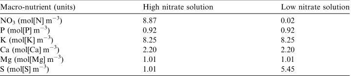
ppm) during both experiments.Table 2shows the concentrations of the

treatment pond was maintained at approximately 9 mol[N] m3[water] (125 ppm) throughout the experiment. For the L treatment pond, 25 ml of stock solution were

added daily, resulting in a nitrate concentration of less than 0.02 mol[N] m3[water]

(0.25 ppm) throughout the experiment. During both experiments, the pH and elec-trical conductivity (EC) in both ponds remained between 5.5–6.5 and 1900–2300

lS cm1, respectively.

Eleven days after sowing into a peat-vermiculite mix in 3 cm plastic cubes, the let-tuce plant cubes were transferred from a growth chamber to the greenhouse, and grown for an additional 24 days in the hydroponics ponds. The plants were held in the ponds on polystyrene floats at the following plant densities: days 11–21: 97

plants m2; days 22–35: 38 plants m2. At the time of re-spacing (day 21 after

sow-ing), half of the plants in the H treatment pond were placed in the L treatment pond, and vice-versa. Time-course harvests (8 plants per treatment) were performed on days 11, 21, 22, 24, 26, and 35 after sowing. In order to prevent changes in the

light-ing environment of the test plants, after each harvestÔguard plantsÕwere moved into

the empty spaces left by the harvested plants.

4. Model calibration

4.1. Conversion between model state variables and measurements

In order to compare the model predictions with the measurements, it is necessary

to convert the state variablesMCs,MCr,MCvandMCeinto the measurable quantities:

Table 1

Summary of the environmental conditions

Experiment 1, June 10–July 15, 1999

Experiment 2,

July 15–August 19, 1999

Average solar radiation at canopy level (mol[PAP] m2_d1₎

15.3 16.7

Average daytime air temperature (C) 24.7 25.6 Average nighttime air temperature (C) 20.8 21.5

Average solution temperature (C) 24.3 23.9

Table 2

Composition of the macro-nutrient in the stock solutions

Macro-nutrient (units) High nitrate solution Low nitrate solution

NO3(mol[N] m3) 8.87 0.02

P (mol[P] m3_{) 0.92 0.92}

K (mol[K] m3_{) 8.25 8.25}

Ca (mol[Ca] m3_{) 2.20 2.20}

Mg (mol[Mg] m3_{) 1.01 1.01}

root and shoot fresh mass, root and shoot dry mass, nitrate concentration and reduced-N content.

Under assumptions similar to those made byLinker et al. (2004), the dry mass

(kg[DM] plant1) can be approximated as

ODM¼

1

N½aCðMCsþMCrþMCvþMCeÞ þaNMNv; ð27Þ

where

aC¼0:03 kg½DM mol1½C and aN¼0:10 kg½DMmol1½N: ð28Þ

In order to obtain separately shoot and root dry mass, it is necessary to make an assumption regarding the distribution of content of the excess-C compartment and the vacuole between shoot and root. Based on the experimental evidence that the dry matter content of the shoot and root are affected similarly by N-stress (not shown), it is assumed that the excess-C and vacuole compartments are distributed proportionally to the size of the compartments:

ODMs ¼

MCs

MCsþMCr

ODM; ð29Þ

ODMr ¼

MCr

MCsþMCr

ODM; ð30Þ

whereODMsandODMrdenote the shoot and root dry mass, respectively.

The fresh mass (kg[FM] plant1) is obtained by adding the mass of water to the

dry mass:

OFMs¼ODMsþ

qkMCs

N ; ð31Þ

OFMr¼ODMrþ

qkMCr

N ; ð32Þ

whereqis the water density.

From Eqs. (8) and (10), the nitrate concentration on a whole plant basis

(mol[N] kg1[FM]) is

ONv¼

P½ðbCMCvÞ=ðkðMCsþMCrÞÞ

bN

1

q

OFMODM

OFM

; ð33Þ

where the first term is the nitrate concentration expressed in mol[N] m3[H2O], and

the second term is the conversion factor required to express the concentration in

mol[N] kg1[FM].

The reduced nitrogen content on a whole plant basis (mol[N] kg1[DM]) is

ob-tained by dividing the mass of reduced nitrogen (Eqs.(8) and (9)) by the dry mass

ORN ¼

r Mð CsþMCrÞ

aCðMCsþMCrþMCvþMCeÞ þaNMNv

½ : ð34Þ

Note that the new parameters included in these relations (q,aC,aN) are considered as

known constants that require no fitting.

Since there are only four state variables for six measurements, inversion of Eqs.

(29)–(34)is not possible. Instead, the initial model states are determined by

minimiz-ing the fittminimiz-ing error function J (Eq.(42)below) at the initial point.

4.2. Nominal parameter values

The nominal values of the parameters are listed in Appendix A. Most of the

parameters related to the shoot and vacuole compartments (and associated fluxes)

are similar to the ones used byLinker et al. (2004), whose model is similar but does

not include a root compartment. The exceptions aree(photosynthetic activity, Eq.

(A.7)) andn(interpolation parameter that determines what fraction of excess carbon

is stored, Eqs.(A.1)–(A.3)), which were changed based on preliminary simulations.

Nominal values for the parameters related to nitrogen uptake, were obtained fromSwiader and Freiji (1996), who used data from nitrate-depletion experiments with lettuce to calibrate a Michaelis-Menten model of the form:

U ¼Imax

CNnC

KþðCNnCÞ

; ð35Þ

whereImaxis the maximum uptake rate. They reported the following ranges for the

parametersC*,K, andImax:

C:½0:4–0:8 106 mol½Nl1½H2O;

K :½7–12 106mol½Nl1½H2O;

Imax:½45–75 109 mol½Ng1½root DMs1:

The very low values ofC* led us to set this term to zero in Eq. (26). The nominal

value ofKwas chosen as 10·106mol[N] l1[H2O].

Under some assumptions, Imax can be used to estimate the product/ar. For a

small root, Eq.(A.12)can be approximated as

frfMCrg arMCr: ð36Þ

At high nitrate concentration and a temperature close toT*, using Eq.(A.10), Eq.

(26)becomes

u/k ð37Þ

and from Eqs.(25), (36) and (37),

which can be rewritten as

FS_Nu /kar

1

aC

aCMCr

½ : ð39Þ

The first bracketed term has the units of mol[N] kg1[DM root] s1, and is

equiva-lent toImax. Using this relation with the nominal value of the parameter k,aCas

gi-ven in Eq.(28), and choosingImaxequal to 50·109mol[N] g1[root DM] s1gives

/ar¼6106 mol½Nmol1½C s1: ð40Þ

Nominal values of the remaining parameters,br,sr,mr, were found by trial-and-error,

leading to the values given inAppendix A.

4.3. Selection of the parameters to be adjusted

Altogether, the model has 21 independent parameters (P(Eq.(11)) andT* (Eq.

(A.10)) can be eliminated), and such a large number of parameters cannot be esti-mated with the limited amount of data available. Therefore, the sensitivity-based

methodology described byIoslovich et al. (2004), and used byLinker et al. (2004),

has been used to select and estimate the parameters to which the model predictions are most sensitive.

Inspection of the experimental data before proceeding with the calibration proce-dure showed that the ratio of water content to reduced-N content was approximately

equal to 7.1 kg[H2O] mol1[N] for all the treatments, which is similar to the data

pre-sented bySeginer (2003)andLinker et al. (2004). From Eqs.(8)–(10), the water

con-tent to reduced-N concon-tent ratio in the model is

V

MNsþMNr

¼k

r: ð41Þ

Therefore, all the subsequent calculations were done imposing the ratiok/requal to

7.1 kg[H2O] mol1[N], and including onlykin the calibration procedure.

4.4. Choice of the fitting error function

J ¼ X

i

OFMsiHFMsi

ð Þ

HFMsi

2

þ ðODMCiHDMCiÞ

Href_DMC

" #2

þ ðORSRiHRSRiÞ

Href_RSR

" #2

8 < : 8 < :

þ ðONviHNviÞ

Href Nv

" #29

= ;

9 = ;

1=2

; ð42Þ

whereOFMs,ODM,ORSRandONvare the shoot fresh mass, dry matter content,

root-to-shoot ratio and vacuolar nitrate concentration calculated from the model

predic-tions, and HFMs, HDM, HRSR and HNv are the corresponding measurements. The

summation (indexi) is performed over all the data points available. Note that for

the fresh mass, which is an accumulating variable and increases almost exponentially with time, the relative error is used. For dry matter content, root-to-shoot ratio and nitrate concentration, which vary over a much narrower range, the error is

normal-ized with respect to a fixed reference given inAppendix A.

5. Calibration results

Starting from the set of nominal parameters given inAppendix A, the method of

Ioslovich et al. (2004)was used to determine which parameters should be further

ad-justed. This procedure resulted in adjusting five parameters, as shown inTable 3.

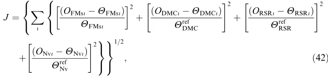
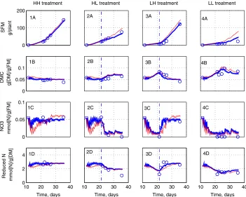
Figs. 2 and 3compare the measurements and predictions of the model for the four treatments of both experiments. For the HH treatments (Frames 1A–1E), growth is almost exponential, with a slow decrease of the RSR and very slow decrease of DMC. Nitrate concentration and reduced-N content remain almost constant. For the HL treatment (Frames 2A–2E), the experimental results are similar to those

gen-erally reported for depletion experiments (Burns, 1992, 1994b;Broadley et al., 2000;

Walker et al., 2001): rapid nitrate depletion, increase of the RSR, slow increase of the DMC, and slow decrease of the reduced-N content. For the LH treatment (Frames 3A–3E), the renewed nitrogen supply causes a sudden increase of shoot growth, accompanied by a reduction of the RSR. Nitrate concentration increases rapidly, while reduced-N content and DMC adjust more slowly. The LL treatment results

Table 3

Results of the calibration procedure

Parameters to be fitted (by decreasing sensitivities) Parameter value Error function (J)

Initial Final Initial Final

bp 0.95 0.84

bN 6.00 8.25

k 0.25·106 0.26·106 0.81 0.50

mr 6.00 7.28

in very small shoot, very high RSR, high DMC, and no vacuolar nitrate (Frames 4A–4E). Overall, the model predictions fit rather well the experimental data.

6. Discussion

6.1. Effects of supply and demand

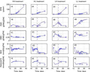
The effects of supply and demand on growth and internal composition are illus-trated by simulations of the HH and the HL treatments of the first experiment.

Fig. 4shows the results for the HH treatment. The sudden jumps in the fluxes on Day 21 correspond to re-spacing of the plants. Frame A shows the potential nitrogen

supply (Eq.(25)) and nitrogen demand (which can be obtained from Eqs.(8), (9),

(A.5) and (A.6)). The actual nitrogen uptake (not shown for clarity) is the smaller of the two. The daily fluctuations of nitrogen demand are due to the fluctuations

0 100 200

HH treatment

SFM g/plant

0 0.5 1

RSR g[DM]/g[DM]

0 0.05 0.1

DMC g[DM]/g[FM]

0 0.05 0.1

NO3 mmol[N]/g[FM]

10 20 30 40 0

5

Time, days

Reduced N mmol[N]/g[DM]

HL treatment

10 20 30 40 Time, days

LH treatment

10 20 30 40 Time, days

LL treatment

10 20 30 40 Time, days 1A

1B

1C

1D

1E

2A

2B

2C

2D

2E

3A

3B

3C

3D

3E

4A

4B

4C

4D

4E

of photosynthesis. Since nitrogen is abundant in the nutrient solution, nitrogen sup-ply is only a function of the root size, and increases monotonically (jump on Day 21 due to re-spacing). Carbon content is low throughout the simulation (Frame B), which indicates that the product of photosynthesis can be used almost immediately

for structural growth. Throughout the simulation, diurnal fluctuations of CCv are

visible, as some carbohydrates are stored in the vacuole during the day, and trans-ferred to the structure at night. Frame C shows that the root carbon demand and the actual flux to the root compartment coincide. The fluctuations of the carbon de-mand are due to fluctuations of the vacuolar carbon content, which is close to the

inhibition level,br(Eqs.(A.6) and (A.15)). Whenever carbon content increases, root

growth inhibition decreases, and root carbon demand increases. Frame D shows the shoot carbon demand and actual flux, and it can be seen that the demand can be sat-isfied at all times.

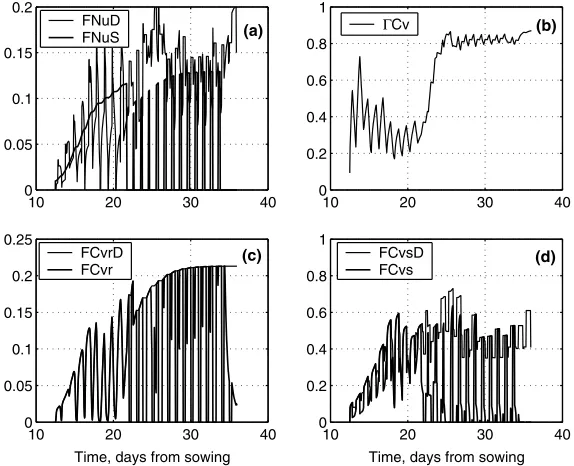
Fig. 5is similar toFig. 4, but for the HL treatment. Up to Day 21, the results are

identical toFig. 4. Following the switch to the low nitrogen solution on Day 21, only

a small quantity of nitrogen is available, immediately after the daily addition of stock solution (Frame A). Vacuolar nitrate is rapidly depleted and replaced by vacuolar

10 20 30 40

0 100 200

HH treatment

SFM g/plant

10 20 30 40

0 0.5 1

RSR g[DM]/g[DM]

10 20 30 40

0 0.05 0.1 DMC g[DM]/g[FM] 0 0.05 0.1

NO3 mmol[N]/g[FM]

10 20 30 40

0 5

Time, days

Reduced N mmol[N]/g[DM]

HL treatment

10 20 30 40

Time, days

LH treatment

10 20 30 40

Time, days

LL treatment

10 20 30 40

Time, days 1A 1B 1C 1D 1E 2A 2B 2C 2D 2E 3A 3B 3C 3D 3E 4A 4B 4C 4D 4E

carbon (Frame B). As a result of vacuolar nitrate depletion, root growth is no longer inhibited, and root carbon demand increases (Frame C). Frame D shows that only very little carbon is available for shoot growth, except immediately after the daily addition of stock solution. Comparison of Frames C and D shows that during the N-stress period, more carbon is transferred to the root than to the shoot, leading to an increased root-to-shoot ratio. Starting on Day 21, some carbon that can not be matched with nitrogen is transferred to the excess-C compartment (not shown),

causing the slow changes of DMC and reduced-N content visible in Figs. 2 and 3

(Frames 2C and 2E).

6.2. Comparison with model with constant root-to-shoot ratio

In order to estimate whether proper modeling of root–shoot partitioning is critical for predicting the effect of nitrogen stress on shoot growth and nitrate concentration, a model with a constant RSR was calibrated. The constant RSR was obtained by

discarding Eqs.(21), (22), (A.6), (A.9) and (A.15), and imposing

FD

Cvs

FD

Cvr

¼FCvs

FCvr

¼R ð43Þ

10 20 30 40

0 0.05 0.1 0.15 0.2

FNuD FNuS

10 20 30 40

0 0.2 0.4 0.6 0.8 1

ΓCv

10 20 30 40

0 0.05 0.1 0.15 0.2 0.25

Time, days from sowing FCvrD

FCvr

10 20 30 40

0 0.2 0.4 0.6 0.8 1

Time, days from sowing FCvsD

FCvs

(a) (b)

(d) (c)

regardless of the status of the crop. The model was calibrated following the

pro-cedure described in Section 4, treating the ratio R as a free parameter (nominal

value: 0.1), and removing the term relative to RSR from the fitting error function

(Eq.(42)). The results of the calibration are summarized inTable 4. The values of

the parameters and error function are only slightly affected by the calibration pro-cedure. For comparison, the error function obtained for the model with a variable

RSR, but excluding the RSR term in Eq.(42), is 0.32. This seems to indicate that

the fitting is greatly improved by a variable root-to-shoot ratio. However,Fig. 6,

which presents the predictions of both models for the second experiment, shows that the predictions differ mainly for the fresh mass of the LL treatment. For all the other treatments, a fixed RSR has almost no effect on the predictions of shoot fresh mass, DMC, nitrate concentration and reduced-N content. Similar

10 20 30 40

0 0.05 0.1 0.15 0.2

FNuD FNuS

10 20 30 40

0 0.2 0.4 0.6 0.8 1

ΓCv

10 20 30 40

0 0.05 0.1 0.15 0.2 0.25

Time, days from sowing FCvrD

FCvr

10 20 30 40

0 0.2 0.4 0.6 0.8 1

Time, days from sowing FCvsD

FCvs

(a) (b)

(c) (d)

Fig. 5. Simulation results for the HL treatment of the first experiment. Frame definitions as inFig. 4.

Table 4

Results of the calibration procedure for the model with constant root-to-shoot ratio

Parameters to be fitted (by decreasing sensitivity) Parameter value Error function (J)

Initial Final Initial Final

bp 0.95 0.91

K 0.25·106 0.26·106 0.76 0.71

results were obtained for the first experiment (not shown). It may therefore be concluded that incorporating a root compartment, and the associated root–shoot partitioning mechanism, is not justified for applications that do not require predic-tion of the root mass, unless plants are N-deprived throughout the whole growing period.

7. Conclusion

The results of this study indicate that, as first claimed byThornley (1972), root–

shoot partitioning can be modeled by source–sink relationships, without explicitly invoking optimization processes. While the priority-based partitioning adopted may be overly simplistic, it proved sufficient to obtain a useful model based on the experimental data available.

Imposing a constant root-to-shoot ratio had almost no consequence on the pre-dictions of shoot fresh mass, dry matter content, nitrate concentration, and

0 100 200

HH treatment

SFM g/plant

0 0.05 0.1

DMC g[DM]/g[FM]

0 0.05 0.1

NO3 mmol[N]/g[FM]

10 20 30 40

0 2 4

Time, days

Reduced N mmol[N]/g[DM]

HL treatment

10 20 30 40

Time, days

LH treatment

10 20 30 40

Time, days

LL treatment

10 20 30 40

Time, days 1A

1B

1C

1D

2A

2B

2C

2D

3A

3B

3C

3D

4A

4B

4C

4D

reduced nitrogen content, except in the extreme case where almost no nitrogen was supplied for the whole growing period. This indicates that for applications in which prediction of the root mass (or equivalently, the root-to-shoot ratio) is not re-quired, modeling of the root–shoot partitioning is not necessary. In particular, with respect to ultimate goal of the NiCoLet project (development of growing strategies that ensure acceptable nitrate level with minimal impact on yield), the simpler

Ôshoot-onlyÕmodel described byLinker et al. (2004), should be preferred. For those

applications in which prediction of the root mass is also of interest, the more gen-eral model presented here, which is still relatively simple and includes only four state variables, should be used.

Acknowledgement

This research has been funded by the European Community, Project FAIR6-CT98-4362 (NiCoLet). Part of this work was achieved during Dr. Linker post-doc-torate in the Biological and Environmental Engineering Department at Cornell University, and the financial support of his host, Prof. L. Albright, is acknowledged.

Appendix A. Notations

Main symbols

aj exponent of effective size of compartmentj, m2[ground] mol1[C]

bk growth inhibition border of processk, dimensionless

CJj concentration of constituent Jin compartmentj, mol[J] m3

C* minimum nitrogen concentration for uptake, mol[N] m3[H2O]

C exponent in respiration equation (A.10), K1

e{Tj} maintenance respiration rate in compartmentj, mol[C] m2[ground] s1

FCk respiration rate of process k, mol[C] m2[ground] s1

FJij flux of constituent J from compartment i to compartment j,

mol[J] m2[ground] s1

FNu nitrogen uptake rate, mol[N] m2[ground] s1

fi{MCi} metabolically active fraction of compartmenti, dimensionless

G a collection of parameters, m3[H2O] Pa mol1[C]

gj{Tj} uninhibited growth rate on compartmentj, mol[C] m2[ground] s1

hj{CCv} inhibition function for compartment j (hj= 1 when no inhibition),

dimensionless

Imax maximum nitrogen uptake rate, mol[N] kg1[DM root]1s1

J fitting error function, dimensionless

K Michalis–Menten coefficient for nitrogen uptake, mol[N] m3[H2O]

k maintenance respiration rate at T=T*, mol[C] m2[ground] s1

MJj molar mass of constituentJin compartment j, mol[J] m2[ground]

N plant density plant, m2[ground]

Olm model outputl,mth measurement, #

p{L,CCa} uninhibited gross photosynthesis of a closed canopy,

mol[C] m2[ground] s1

R root-to-shoot ratio

r N to C ratio in structure, mol[N] mol1[C]

sj growth inhibition slope for compartmentj

Tj temperature of compartmentj, K

T* reference temperature, K

t time, s

U nitrogen uptake rate (Eq.(35)), mol[N] kg1[root DM] s1

u{Tn,CNn} potential nitrogen uptake rate, mol[N] m2[ground] s1

V volume of water, m3[H2O] m

2

[ground]

aJ contribution ofJto dry mass, kg[DM] mol

1

[J]

bJ osmotic pressure associated with one unit of vacuolar J,

m3[H2O]Pa mol1[J]

e photosynthetic efficiency, mol[C] mol1[PAP]

CJv normalizedJ-concentration in vacuole, dimensionless

/ potential uptake rate at non-limiting concentration, mol[N] mol1[C]

k volume of water associated with one unit of structural, C m3[H2O] mol1

[C]

mj ratiogj{Tj}/e{Tj}, dimensionless

P osmotic pressure in vacuole, Pa

Hlm measured outputl,mth measurement, #

h growth respiration as fraction of growth, dimensionless

q water density, kg m3

r leaf conductance to CO2, m s1

n interpolation parameter, dimensionless

Note.# indicates that the units depend on the output l

Subscripts

Compartments

a atmosphere

e excess carbon

i,j general compartment indices

n nutrient solution

r root

s shoot

Constituents

C carbon

J general constituent index

Processes

g growth respiration

m maintenance respiration

p photosynthesis

Outputs

DM dry mass

DMC dry mass content

DMr dry mass root

DMs dry mass shoot

Nv vacuolar nitrate

RN reduced nitrogen

RSR root-to-shoot ratio

Superscripts

D determined by crop demand

ref reference

S potential supply rate

Acronyms

DM dry mass

DMC dry matter content

FM fresh mass

PAP photosynthetically active photons

SFM shoot fresh mass

A.1. Carbon fluxes

The carbon fluxes that form the RHS of Eq.(15)are formulated as:

FCp¼pfL;CCagfsfMCsg½nþ ð1nÞhpfCCvg; ðA:1Þ

FCve¼pfL;CCagfsfMCsg½ð1hpfCCvgÞn; ðA:2Þ

FCev¼gsfTagfsfMCsg½ð1þhÞð1hsfCCvgÞn þ grfTngfrfMCrg

½ð1þhÞð1hrfCCvgÞn;

ðA:3Þ

FCm¼efTagfsfMCsg þe Tf ngfrfMCrg ðA:4Þ

and the carbon demand of the shoot and root compartments is formulated as

FD

Cvr¼grfTngfrfMCrghrfCCvg: ðA:6Þ

The fluxes defined by Eqs.(A.1)–(A.4) are functions of the environment (light, L;

temperatures,TaandTn; CO2concentration,CCa), and the state of the crop (MCs,

MCr,CCv). The parametern, which appears in Eqs.(A.1)–(A.3), is an interpolation

parameter (between 0 and 1), and controls the degree to which photosynthesis is

af-fected by the inhibition functionhp.

The fluxes of potential gross photosynthesis and growth are formulated as

pfL;CCag ¼

eLrCCa

eLþrCCa

; ðA:7Þ

g_sfTag ¼msefTag; ðA:8Þ

g_rfTag ¼mrefTng; ðA:9Þ

where

efTg ¼kexpfcðTTÞg: ðA:10Þ

is the photosynthetic efficiency,ris the conductance to CO2,kis the maintenance

respiration rate atT* and mr,ms andcare constant coefficients.

The effect of crop size on the fluxes is modeled as

fsfMCsg ¼1expfasMCsg; ðA:11Þ

frfMCrg ¼1expfarMCrg; ðA:12Þ

asis a light extinction coefficient, so thatfs{MCs} may be considered as representing

the metabolically active part of the shoot (Seginer, 2003). fs{MCs} equals 1 for a

closed canopy which absorbs all the light available. TheÔactiveÕroot size is modeled

similarly, because old roots apparently do not contribute greatly to nitrogen uptake.

The inhibition functionshp,hrandhs are formulated as:

hpfCCvg ¼

1

1þ ₁1_Cbp

Cv

sp; ðA:13Þ

hsfCCvg ¼

1

1þ bs

CCv

ss; ðA:14Þ

hrfCCvg ¼

1

1þ br

CCv

wherebr,bs,bp,sr,ssandspcontrol the shape of the inhibition functions.

Photosyn-thesis inhibition,hp, approaches zero as vacuolar nitrate is depleted, and increases

asymptotically to 1 with increasing vacuolar nitrate content. The interpretation of

hpdepends on the value ofn. Whennequals 0, which corresponds to a model

with-out an excess-C compartment,hp inhibits photosynthesis. When 0 <n61,

photo-synthesis is only partially inhibited (no inhibition when n= 1), and hp acts as a

partitioning function that diverts a fraction of the carbon to the excess-C

compart-ment.hrandhsrestrict the transfer of carbon from the vacuole to the root and shoot

when vacuolar carbon is scarce, and are qualitatively mirror images ofhp.hrinhibits

root growth when vacuolar nitrate content is high, since in such a situation there is

no need to increase the nitrogen uptake capacity of the plant. hs inhibits shoot

growth when vacuolar carbon is scarce. The relative positions ofhp,hrandhsshould

be such that when vacuolar nitrate is abundant, root growth is inhibited before shoot growth.

Nominal values of the parameters

ar 4 m2[ground] mol1[C]

as 1.7 m2[ground] mol1[C]

br 0.3

bs 0.2

bp 0.95

K 10·106mol[N] m3[H2O]

k 0.25·106mol[C] m2[ground] s1

R 0.1

sr 10

ss 10

sp 10

T* 20C

bC 0.6 m

3

kPa mol1[C]

bN 6.0 m

3

kPa mol1[N]

7.5·103mol[C] mol1[PAP]

/ 1.5·106mol[N] m2s1

k 0.75·103m3[H2O] mol1[C]

mr 6

ms 20

P 580 kPa

h 0.3

r 1.4·103m s1

n 0.7

Values of the parameters used for unit conversions

aC 0.03 kg[DM] mol1[C]

Normalization values used in the error function (Eq.(42))

HDMCref 0.05 kg[DM] kg1[FM]

HRSRref0.25 kg[root DM] kg1[shoot DM]

HVNref 0.01 mol[N] kg1[FM]

References

A˚ gren, G.I., Ingestad, T., 1987. Root:shoot ratio as a balance between nitrogen productivity and photosynthesis. Plant, Cell and Environment 10, 579–586.

Albright, A., Both, A.J., Chiu, A.J., 2000. Controlling greenhouse light to a consistent daily integral. Transactions of the ASAE 43, 421–431.

Behr, U., Wiebe, H.J., 1988. Relations between nitrate content and other osmotica in the cell sap of lettuce cultivars (Lactuca sativaL.). Gartenbauwissenschaft 53, 206–210.

Blom-Zandstra, M., Lampe, J.E.M., 1985. The role of nitrate in the osmoregulation of lettuce (Lactuca sativaL.) grown at different light intensities. Journal of Experimental Botany 36, 1043–1052. Blom-Zandstra, M., Lampe, J.E.M., Ammerlaan, F.H.M., 1988. C and N utilization of two lettuce

genotypes during growth under non-varying light conditions and after changing the light intensity. Physiologia Plantarum 74, 147–153.

Broadley, M.R., Escobar-Gutierez, A.J., Burns, A., Burns, I.G., 2000. What are the effects of nitrogen deficiency on growth components of lettuce?. New Phytologist 147, 519–526.

Burns, I.G., 1992. Influence of plant nutrient concentration on growth rate: Use of a nutrient interruption technique to determine critical concentrations of N, P and K in young plants. Plant and Soil 142, 221–233. Burns, I.G., 1994a. Studies of the relationship between the growth rate of young plants and their total-N concentration using nutrient interruption techniques: Theory and experiments. Annals of Botany 74, 143–157.

Burns, I.G., 1994b. A mechanistic theory for the relationship between growth rate and the concentration of nitrate-N or organic-N in young plants derived from nutrient interruption experiments. Annals of Botany 74, 159–172.

Chen, J.L., Reynolds, J.F., Harley, P.C., Tenhunen, J.D., 1993. Coordination theory of leaf distribution in a canopy. Oecologica 93, 63–69.

Gleeson, S.K., 1993. Optimization of tissue nitrogen and root–shoot allocation. Annals of Botany 71, 23– 31.

Hilbert, D.W., 1990. Optimization of plant root:shoot ratios and internal nitrogen concentration. Annals of Botany 66, 91–99.

Ioslovich, I., Seginer, I., 2002. Acceptable nitrate concentration of greenhouse lettuce: two optimal control policies. Biosystems Engineering 83, 199–215.

Ioslovich, I., Gutman, P.O., Seginer, I., 2004. Dominant parameter selection in the marginally identifiable case. Mathematics and Computers in Simulation 65, 127–136.

Johnson, I.R., 1985. A model of partitioning of growth between the shoots and roots of vegetative plants. Annals of Botany 55, 421–431.

Johnson, I.R., Thornley, J.H.M., 1987. A model of shoot:root partitioning with optimal growth. Annals of Botany 60, 133–142.

Linker, R., Seginer, I., Buwalda, F., 2004. Description and calibration of a dynamic model for lettuce grown in a nitrate-limiting environment. Mathematical and Computer Modelling (in press). Lopez Cruz, I.L., van Willigenburg, L.G., van Straten, G., 2003. Optimal control of nitrate in lettuce by a

hybrid approach: differential evolution and adjustable control weight gradient algorithms. Computers and Electronics in Agriculture 40, 179–197.

Macduff, J.H., Jarvis, S.C., Larsson, C.M., Oscarson, P., 1993. Plant growth in relation to the supply and uptake of NO3: A comparison between relative addition rate and external concentration as driving

Makela, A.A., Sievanen, R.P., 1987. Comparison of two shoot-root partitioning models with respect to substrate utilization and functional balance. Annals of Botany 59, 129–140.

Reynolds, J.F., Thornley, J.H.M., 1982. A shoot:root partitioning model. Annals of Botany 49, 585–597. Reynolds, J.F., Chen, J., 1996. Modelling whole-plant allocation in relation to carbon and nitrogen

supply: Coordination versus optimization: Opinion. Plant and Soil 185, 65–74.

Seginer, I., van Straten, G., Buwalda, F., 1999. Lettuce growth limited by nitrate supply. Acta Horticulturae 507, 141–148.

Seginer, I., 2003. A dynamic model for nitrogen stressed lettuce. Annals of Botany 91, 623–635. Swiader, J.M., Freiji, F.G., 1996. Characterizing nitrate uptake in lettuce using very-sensitive ion

chromatography. Journal of Plant Nutrition 19, 15–27.

Tabourel-Tayot, F., Gastal, F., 1998. MecaNiCAL, a supply-demand model of carbon and nitrogen partitioning applied to defoliated grass. 1. Model description and analysis. European Journal of Agronomy 9, 223–241.

Thornley, J.H.M., 1972. A balanced qualitative model for root:shoot ratios in vegetative plants. Annals of Botany 36, 431–441.

Thornley, J.H.M., 1995. Shoot:root allocation with respect to C, N and P: an investigation and comparison of resistance and teleonomic models. Annals of Botany 75, 391–405.

Thornley, J.H.M., 1997. Modelling allocation with transport/conversion processes. Silva Fennica 31, 341– 355.

Thornley, J.H.M., 1998. Modelling shoot-root relations: the only way forward. Annals of Botany 81, 165– 171.