Math 2Z03 – Differential Equations

Math 2Z03 – Differential Equations

By: Kemal Ahmed

June 2013

Integration Hints

Order of by parts

1. Log

2. Inverse Trig 3. Algebraic function 4. Trig

5. Exponential

( )

2 2

2 2 2

3 2

x x u

x x x

e x dx c e x xdx c e udu c y x

e e e

+ ⋅ + +

=

∫

=

∫

=

∫

Euler Shortcut

Remember this incredibly long integration by parts?

∫

excos

( )

x dx?

Well cos

( )

;sin

( )

2 2

ikx ikx ikx ikx

e e e e

kx kx

i

− −

+ −

= = by Euler’s identity, so sub that in and you get:

d 2

ix ix

xe e

e x

i

− +

∫

Or cos

( )

d d

2

ibx ibx

ax axe e

e bx x e x

− + =

∫

∫

Don’t confuse these with hyperbolic trig:

( )

( )

cosh ;sinh

2 2

kx kx kx kx

e e e e

kx x

− −

+ −

= =

Integration by parts shortcut: Tic Tac Toe Method e.g. 3

cos d x x x

∫

1) Choose a u that can be derived, until it becomes 0 (e.g.x3) Put it into the following chart:

Sign of u: always alternate and start positive

Derivatives of u: don’t stop, until you hit 0.

Integrals of v

+ 3

x cosx

− 2

3x sinx

+ 6x −cosx

+ 0 cosx

2) Multiply each derivative of u, including u, by its sign and by the next integral of v and add the terms:

( )

(

) ( )(

) ( )(

)

3 2

sin 3 cos 6 sin 6 cos

x x− x − x + x − x − x +c

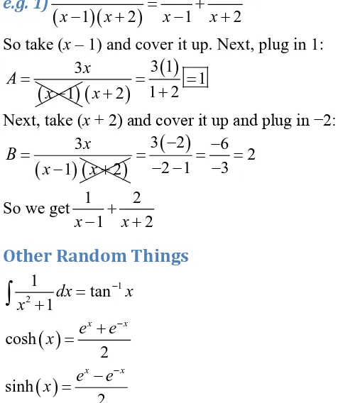
Shortcut: Cover-up method

This only works for linear factors (i.e. power of one). Take each zero in the denominator and “cover up” that factor. Next, plug the factor into this covered up equation to find each letter.

e.g. 1)

₍

₎₍

3

₎

1 2 1 2

x A B

x− x+ = x− + x+

So take (x – 1) and cover it up. Next, plug in 1:

(

)

3 1 x A x = −

(

)

( )

3 1 1 1 2 2

x+ = + =

Next, take (x+ 2) and cover it up and plug in −2:

(

) (

)

3 1 2 x B x x = − +

( )

3 2 6

2

2 1 3

− −

= = =

− − −

So we get 1 2

1 2

x− +x+

Other Random Things

[image:2.612.70.308.213.497.2]

( )

( )

1 2 1 tan 1 cosh 2 sinh 2 x x x x dx x x e e x e e x − − − = + + = − =

∫

Table of Partial Fraction Decompositions

( )

Q x Example Decomposition due to Q x

( )

linear factor

(

_{4 5x+}

)

4 5 A x + Irreducible quadratic factor 2 1 x + 2 1 Ax B x + + Repeated

linear factor

(

)

3 2x−1

(

_{) (}

) (

2

)

3

2 1 _{2 1 2 1}

A B C

x− + _x− + _x− Repeated irreducible

quadratic factor

(

)

2 2

2 x +

(

)

2

2 ₂

2 ₂

Ax B Cx D

x _x

+ ₊ +

(

)

2 2

3

2 2

x A B C

x x x x x

− _{= + +}

+ +

Limit stuff

Nth term test: for 1

1, convergent 1

,

1, divergent

p n

p p n ∞

=

>   ≤ 

∑

0

! n

n n

n

a x n a

∞

=

=

∑

Ratio test: tests for convergence; for

1 1

, lim

n n

n n n

a a

a + ∞

→∞ =

∑

Radius of convergence: I’m just going to show you an example of how it works because I don’t understand it that well, myself.

e.g. 2) Ratio Test

2

1 25 s −

about x = 0

(

s−5

)(

1s+5

)

, then R = 5

e.g. 3) Singular points

(

2

)

25 2 0

x − y′′+ xy′+ =y about x = 1

(

52

)(

5

) (

5

)(

5

)

0

xy y

y

x x x x

′′ + + =

− + − +

Singular points: −5,5

The smallest distance between −5 or 5 and 1 is 4. Therefore R = 4.

Chapter 1 – Introduction to Differential Equations

1.1 − Introduction

Linear Differential Equation: the equation has every order lower than the highest, e.g.

( )

2

( )

( )

( )

2 2 1 0

d d

d d

y y

a x a x a x y g x

x + x+ = , whereas this is non-linear:

( )

2

( )

( )

2 2 1

d d

d d

y y

a x a x g x

x + x=

unnecessarily correct. The reason why is because the italicised things are variables. However, the d is more of a function than a variable and functions are not supposed to be italicised [source].

The differential operator: usually in the form, d

( )

2 2

dx x = x, is a linear operator. It’s also known as Leibniz Notation. ( )

2

2 2

d

'' d

y

y y y

x = = =

Ordinary Linear Differential Equation (ODE): a differential equation with functions of a single variable and their derivatives

Partial Differential Equation (PDE): a differential equation that contains unknown multivariable functions and their partial derivatives

2 2 xx u

u x

∂ ₌

∂ Note: not until Math 2ZZ3.

The order of a differential equation is the order of the highest order derivative in the equation.

Normal form is when you move everything over to the right side of the equation, except the highest order derivative.

Explicit solutions only have a single y that is to the power of 1 and derivative order 0 (i.e.

( )0

y = y). Generally, when converting from an implicit solution (not explicit) to an explicit solution, there are as many solutions as there are powers. For example, when converting the

equation of a circle, 2 2 2

x +y =r , to explicit, you get 2 solutions: 2 2

y= + r −x and 2 2

y= − r −x .

Verification of a solution:

Particular Solution: what you get after you put values into all the constants in an explicit solution

General Solution: explicit solution before plugging in constants to the complementary solution.

Implicit Differentiation: a verification method for implicit solutions that involves

differentiating with respect to the independent variable (usually x). e.g. 1.1 example 3: prove

2 2

25

x +y = is a solution of the differential equation, d_dy x

x = −y on the interval, −5 < x < 5.

Implicit differentiation demands that you first differentiate with respect to x, so

d d

2 2

d d d 2

d d d 25 2 2 d 0 d 2

y y x x

xx xy x x y x x y y

−

+ = ⇒ + = ⇒ = = −

1.2 – Initial-value Problems

Solution to differential equation: just a nice function without derivatives (i.e. no y’, y”, etc., just y = …)

Initial conditions: a point that is part of the solution

Initial Value Problem (IVP): when initial conditions from only one input are given. They can give outputs to your solution and/or derivatives of your solution. This helps you determine the constant after integration gives you your family of solutions that gives you your specified solution.

When you havey=ex c+ , it’s easier if you replace it like this:

0, where must be positive0

x c

x c

x

y e

y e e

y e y y

+ = = ⋅ = ⋅

N-order differential equation: can be broken up into n first-order differential equations, so it gives n solutions (because n constants from n integrations). Gives an n-parameter family of solutions.

Direction Field = Slope field:

Second-order differential equation: 2 solutions for each given initial condition

IVP versus BVP: IVP has 1 point, BVP has multiple points

When you have constant coefficients (i.e. no coefficients are x’s) and a linear equation, you may always guess rx

y=e , so for ay''+by'+cy=0, you get 2

0

rx rx rx

ar e +bre +ce = , since derivative of rx

e is rx

re , etc. Since erx >0, it cannot be the part of the terms that allows it to equal 0, so you can just take it out, giving you 2

0 ar +br+ =c .

Bernoulli

When you have a power of y in the g(x), you need to use Bernoulli’s equation: 1. Divide both sides by the y term in the g(x). Let’s call the termyn.

2. Let v= yn−1

3. Differentiate to getv'= −

(

1 n y y

)

−n '.

4. Plug v & v’ into the equation to get 1

( )

( )

1−nv'+P x v=Q x .

5. Solve the DE for v(x).

Chapter 2 – First Order Differential Equations

2.1 – Solution curves Without a Solution

Direction fields: play around with different points!

2.2 – Separable Equation

Bring all the y’s and orders and powers of y to one side and bring all the x’s and orders and powers of x to one side. Integrate both sides.

( )

dy

( )

( )

( )

dx

N y =M x →

∫

N y dy=

∫

M x dx

When given a circle, keep in mind that the slope of all lines isy_x. Since the slope at each point of the circle is perpendicular to the previous (recall inward acceleration),d_dy x

x = −y, the negative

reciprocal of y_x.

2.3 – Linear Equations

Integrating Factor:

( )

( )d

P x x

x e

µ = ∫

1. Put your equation into the following form:y'+P x y

( )

=Q x

( )

, where there are no coefficients in front of the y’. This is also known as standard form.

2. Find the integrating factor.

3. Without showing proof:

( )

( ) ( )

( )

d x Q x x c y t

x µ

µ

+ =

∫

If Q(x) = 0, treat as a separable equation.

Transient terms are terms in the solution with constants in them. 2.7 – Linear Models

The general formula for growth and decay is d

( )

₀

d

kt x

kx P t P e

t = → = , where k is the

growth/decay constant.

Newton’s Cooling Law: d

(

)

;

d

kt

m m m

T

k T T T T ce T

t = − → = + =ambient temperature, the

temperature of the medium around the object.

2.8 – Nonlinear Models

Logistic Equation:d

d

P r

P r P

t K

 

= _ − _

Chapter 3 – Higher-Order Differential Equations

3.1 – Theory of Linear Equations

Homogeneous: in short g(x) = 0 means homo; g(x) ≠ 0 means no-homo 1. 2 '' 3 'y + y+ =y 0is homogeneous

2. 2 '' 3 'y + y+ + =y 1 0is nothomogeneous because you can bring the −1 to the other side and then the equation equals −1, not 0.

3. 2

3xy' 3− x y=7xis not homogeneous because you have 7x is not 0.

Homogeneous equation (get into this form): a_n

( )

x y( )n +a_n−1

( )

x y( )n−1 + +... a x y₁

( )

'+a₀

( )

x y=0 No-homo equation: a_n

( )

x y( )n +a_n−1

( )

x y( )n−1 + +... a x y₁

( )

'+a₀

( )

x y=g x

( )

Over-determined: more than n different conditions for n-order BVP

Under-determined: less than n different conditions for n-order BVP

For homo equations, your general solutionis your complementary solution and the particular solution is what you get when you plug in values and find the constants from the

complementary solution. I.e. Whenever the right side is 0, your only solution is the complementary solution.

Synthetic Division / Horner’s Rule

This is a method that lets you find the factors in an equation. In this course, we’ll use it to find the roots in an auxiliary equation. Given a function, sayax3+bx2+cx+ =d 0, guess a number that is a factor of d

a

± (you may be given bigger powers, in which case you still use the first and last numbers).

3.3 – Homogeneous Linear Equations with Constant Coefficients

Auxiliary Equation

Auxiliary equation: gives complementary solution (a.k.a. associated solution).

1. Take a differential equation and divide everything by the coefficients in front of the highest power of x, which makes the right side g(x).

2. Guess y=emx ⇒y'=memx ⇒ y"=m e2 mx ⇒etc. 3. Assume the right side equal to 0 for now. 4. Divide everything byemx.

5. Factor out your roots.

For real, distinct roots: 1 2

1 2 etc.

r x r x

c

y =c e +c e +

For repeated roots: multiply repeats byxrepeats 1− , i.e. y_c =c e₁ mx+c xe₂ mx

For complex roots (a ± bi): yc =eax

(

c₁cos

( )

bx +c₂sin

( )

bx

)

For non-constant coefficients, see chapter 5, unless the powers of the x’s are the same as the order of the y they are multiplied by, where you would use Cauchy-Euler.

3.4 – Undetermined Coefficients

Most of the time, the general solution of a problem is the complementary solution + the

particular solution.

This method finds you the particular solution. It is usually preceded by Cauchy−Euler or

auxiliary because you must find the complementary solution to know if you have any repeats. g(x), the right side of equation Particular solution guess (y)

t

aeβ Aeβt

( )

cos

a βt Acos

( )

βt +Bsin

( )

βt

( )

sin

b βt Acos

( )

βt +Bsin

( )

βt

( )

( )

cos sin

a βt +b βt Acos

( )

βt +Bsin

( )

βt

nth degree polynomial 1

1 1 0

n n

n n

A t +A t₋ − + + A t+A

Else Go to Variation of Parameters. Plug in your guess into your differential (i.e. differentiate for all the orders, too). If the left side becomes 0, you bump up the guess. That means you multiply your guess by x. So Ax + B becomesAx2+Bx.

If you have roots that are the same as roots from the complementary solution, you also need to bump up the guess.

Modified Undetermined Coefficients

This is meant to make Undetermined Coefficients work for Cauchy-Euler, but also works for the regular auxiliary method.

1. Represent all x’s in the right side of the equation byet. 3.5 – Variation of Parameters

This method finds the particular solution. It is usually preceded by Cauchy−Euler or auxiliary

because the method uses the complementary solutions when finding the Wronskians. 1. Extract solutionsy y₁, ₂, etc.from your complementary solution. E.g. if your

complementary solution is y_c =c e₁ tcos 3

( )

t +c e₂ tsin 3

( )

t , youry₁ =eaxcos

( )

bx , and

( )

2 sin

ax

y =e bx

2. Put your equation in standard form so you have the correct g(x) (i.e. no non-constants in front of highest order y).

3.

( )

2 1

2 0 W

' y g x y

= ,

( )

1

2 1

0 W

' y

y g x

= ,

(

_{1 2}

)

1 2

1 2

W ,

' '

y y y y

y y

= , 1

1

W '

W

µ = , 2

2

W '

W

4. Shortcut:

( )

(

)

(

( )

)

2 1

particular 1 2

1 2 1 2

d d

W , W ,

y g x y g x

y y x y x

y y y y

= −

∫

+

∫

5. Also, ignore the constants you get from the integration.

3.6 – Cauchy-Euler Equation

Cauchy-Euler gives you the complementary solution. You know something is a Cauchy-Euler because the powers of the x’s are the same as the orders of the y derivatives they are multiplied by. Pretend the g(x) = 0 for now. Next, guess 1

(

)

2

' " 1 etc.

m m m

y=x ⇒ y =mx − ⇒ y =m m− x − ⇒

This may look weird at first, but the xmwill still end up cancelling out. Factor the m’s and find the roots.

Distinct, real roots: 1 2

1, 2: 1 2

m m

m m y=c x +c x

Repeated roots: 1 1 1

( )

2 2

1, 1, 1, 2: 1 2 ln 3 ln 4

m m m m

m m m m y=c x +c x x c x+ x +c x Complex roots: m_1,2

(

a bi±

)

:y=xa

(

c₁cos

(

blnx

)

+c₂sin

(

blnx

)

)

This is usually followed by Variation of Parameters because it’s easier. However, there is a

modified method of Undetermined Coefficients that also works.

Sometimes, you may have to multiply both sides by x to be able to use this method. For example,

" ' 0 xy +y = .

When you end up with complex values of m, you need to solve using boundary value problems. 3.8 – Linear Models: IVPs

Note: this is not for a system of linear equations. That is chapter 5.

Springs, dampening, other fun

2

; 2 k

m m

β

ω = λ = ,β = positive damping constant

Un-damped motion:

( )

( )

( )

2 2

1 2

2

d

0 cos sin

d x

x x t c t c t

t +ω = → = ω + ω

Damped motion: 2

2 2

d d

2 0

d d

x x

x

t + λ t +ω =

Over-damped:λ2−ω2 >0, so no i,

( )

1 2

1 2

m t m t

x t =c e +c e

Critically:λ2−ω2 =_{0;x t}

( )

=_e−λt c(1+c t2)

Under: 2 2 0;

( )

(

1cos

(

2 2

)

2sin

(

2 2

)

)

t

x t e λ c t c t

λ ₋ω _{< =} − ω ₋λ ₊ ω ₋λ

3.9 – Linear Models: BVPs

When you end up with complex values of m, you need to solve using eigenfunctions. The

method is supposed to focus on what you get after you find your values of m. The following is an explanation of the example on page 161 of your textbook.

e.g. y"+λy=0,y

( )

0 =0, 'y

( )

π₂ =0

First find yourycthrough auxiliary.

2

0 m

m λ

λ + = = −

Since sin & cos act differently depending on the value of λ, we need to find 3 y’s: one for each case of λ > 0, λ = 0, λ < 0.

Case 1: λ > 0

m= − = ±λ i λ

Since λ is positive, no extra sign, so λ stays negative. We’re going to guess:

( )

( )

1cos 2sin

y=c x λ +c x λ

Ok! Let’s try to findc₁&c₂using initial conditions.

( )

( )

( )

1 2

1 0

1 1

0 0

cos 0 sin 0

0 0

0 y

c c

c

c

λ λ

=

= +

= + =

 

Cool! Now, to try the next initial condition, we need to differentiate. To make it easier, let’s not differentiate the first term, since we already know thatc1=0, and leave it as 0.

( )

( )

( )

2

2

2 2

' 0 cos

' 0

cos

y c x

y

c π

π

λ λ

λ λ

= + = =

Now bun the √λ by dividing it out, which it will nicely, since you have a 0 on the other side. So

you’re left with:c₂cos

( )

π₂ λ =0. Ok, so at this point it looks like we aren’t going to have any equation becausec₁=0and nowc₂might be zero because we know the √λ didn’t make the right side zero from the case (λ > 0). But that doesn’t make sense because the formula has to exist. Therefore, c₂ =1 .

So what’s making it 0? The cos. So now think: what values of cos make cos = 0? You guessed

(

2n 1

)

2

π

+ , right? Yeah! You got it right. Ok, so equate that to what’s already inside the cos:

2

π

(

)

2

2n 1 π

λ = + ⇒ λ =2n+1

Case 2: λ = 0

Plugging λ = 0 into our initial formula gives us y” = 0 Integrate this twice and get y= +c₁ c x₂

( )

2

1 1

0 0

' 0 0

y c

y c x y c y

= =

= ⇒ = = ⇒ =

Case 3: λ < 0 since is

negative m= − λ λ → λ

Playing around with c₁gives:y=c₁cosh

( )

x λ +c₂sinh

( )

x λ Sub in the initial conditions:y

( )

0 = =0 c₁

( )

1 +c₂

( )

0

1 0

c = ←sub this into the cosh shit and you make the cosh shit 0, so you’re left with

( )

( )

( )

( )

2 2

2

2 2

sinh

' cosh

' cosh 0

y c x

y c x

y π c π

λ

λ λ

λ λ

=

=

= =

Now think about the last line. What part of it made it zero? The hyperbolic cosine will never equal 0, so it can’t be that. The λ has already been established to be less than (and not equal to) zero, so it can’t be that either. Thus, you can say that the part making it 0 is the constant.

2 0 0 c

y ∴ = ∴ =

Wasn’t that fun? We went through all 3 cases. Yeah, I know. We could have just stopped at the first case, smiled, and continued with our arduous quest to find the Math Magician (reference to Math Journey video game by the Learning Company), but I decided to show you all 3 cases in case you do come across a problem that requires any of the other cases.

Chapter 8

− Matrices

8.8 – Eigenvalues and Eigenvectors The definition of an eigenvalue

The eigenvalues are the zeroes you get by isolating λ from the equation,

(

)

(

)

det λI−A =det A−λI =0, where I is the identity matrix of size n. The identity matrix of a given size is a diagonal matrix of all ones.

Ak = λk (A−λI)k = 0

e.g. of eigenvalues

For a matrix, 6 3 2 1 A=  _

 , the eigenvalues are

(

)(

)

1 2

0

6 3

6 1 6

7

2 1

λ λ

λ λ

λ λ

= −

= − − − ⇒

=

Matrix Properties

( )

T _{T T}

AB =B A

The zero matrix has size, but all zeroes. Note: it is not invertible

Triangle matrix is half zeroes and half full:

1 2 3 4

0 5 6 7

0 0 8 9

0 0 0 10

 

 

 

 

 

 

Diagonal matrix only has values from the top left to bottom right:

1 0 0

0 2 0

0 0 3

 

 

 

 

 

Symmetric matrix:AT = A←always have real eigenvalues

( )

( )

det AT =det A det(A) = 0 if:

• Any 2 rows/columns in A are the same • Any column or row is zero

det(AB) = det(A)∙det(B)

Non-singular: invertible

( )

( ) ( )

1

1 _{1 1}

1 ₁ T

T

AA I AB B A

A A

−

− _{− −}

− ₋

= = =

Regarding the matrix

a b c d e f g h i

 

 

 

 

 

,c₁₁ e f h i

= ,c₁₂ d f

g i

= , i.e. take out the row and column of

the cofactor index. The cofactor matrix would be:

11 12 13 21 22 23 31 32 33

c c c

c c c

c c c

 

 

 

 

 

The adjoint matrix is the transpose of the cofactor matrix. The inverse can be found in 3 ways:

1.

( ) ( )

1 1

adj det

A A

A

− ₌

2. 1

( )

A− = A I and do row echelon until you get

(

I A−1

)

3. A shortcut for size-2 matrices:

( )

1

1 det

a b d b

c d A c a

−

−

   

=

  ₋ 

   

Cramer’s Rule: converts equations to matrices, e.g. ax by e e a b x

cx dy f f c d y

+ =

      

⇒ =

 _{+ =}      

Complex Eigenvalues

When you have complex eigenvalues, it will look scary, but just treat the i like a regular number. Sometimes, when doing row-reduction, you may have to multiply a row by i.

Finding the Eigenvectors

Plug each eigenvalue into A and row reduce.

If 0 9

1 0 A=  _

 , thenλ1=3,λ2 = −3

Then 1 1

1

9 0

1 0

x y λ

λ −

     

=_{     }= − _{   }

 

K

The bottom row should row reduce to 0, so all you’re left with is:

3 9 0

3 9

3 x y

x y

x y

− + =

= − = −

Now let y = 1 and you get: ₁ 3 1 −   =    

K

8.9 – Powers of Matrices (not on exam) Ak =PD Pk −1

1. Use A – λI to find the eigenvalues, e.g. −2, 1, 4 from

2 2 0

4 0 0

1 2 1 A

 

 

=  

 

 

2. Substitute the eigenvalues into the following formula: 2

0 1 2 ...

m n

n

c c c c

λ = + λ+ λ + + λ , where n is the size of the matrix and m is the desired power.

0 1 2

0 1 2

0 1 2

2 2 4

1

4 4 16

m

m

c c c

c c c

c c c

− = − +

= + +

= + +

3. Isolate for the three constants

0 2 1 4 2 2

m

c = c − c −

8.10 – Orthogonal Matrices

The inner product or dot-product of two matrices, x · y =xTy The norm of a matrix, X = X X⋅

The complex conjugate of something, like A, is denoted by A . The conjugate of anything real is itself.

Orthogonality

Let A be an n × n symmetric matrix. Then eigenvectors corresponding to distinct eigenvalues are

orthogonal.

An n × n matrix, A, is said to be orthogonal ifA−1=AT. Therefore, you can prove something is orthogonal by confirmingAAT =I.

An n × n matrix, A is orthogonal if and only if its columns x x₁, ₂,...x_nform an orthonormal set. A set of vectors is called orthonormal if they are distinct, orthogonal, and if each vector is a unit vector.

Creating orthogonal matrices

1. A = [ ] ←get λ

2. Check if all 3 eigenvectors are distinct. If you can’t tell after row reduction, you can check by making sure the inner product is 0.

3. Make it orthonormal by dividing each column vector by its norm 4. Combine into a matrix

8.12 − Diagonalization

Symmetric matrices can always be diagonalized.

Diagonalizable matrices have n distinct eigenvalues, where n is the size of the matrix. 1

D=P AP−

The columns of D are eigenvalues. Therefore, the columns of P are eigenvectors.

Chapter 10 – Systems of Linear Differential Equations

10.1 – Theory of Linear Systems

Blah blah:

10.2 – Homogeneous Linear Systems

x x

y y

′

   

=  _′     A 

When given a linear system: 1. Find eigenvalues

2. Find eigenvectors

General solution: 1 2

1 1 2 2 etc.

t t

y=c eλ K +c eλ K +

Chapter 4 – Laplace Transform

4.1 – Definition of Laplace Transform Definition of Laplace:

{

( )

}

( )

0 d

st

f t =

∫

∞ −e f t t

4.2 – Inverse transform and transforms of derivatives Most of these Laplace formulas are in the back of the book

4.3 – Translation Theorems Heaviside function

(

)

a = t−a

 

4.4 – Additional Operational Properties

Laplace of Derivatives

( )

{

}

3

( )

2

( )

( )

( )

0 0 0

y′′′ t =s Y s −s y −sy′ −y′′



Laplace of Integrals

Convolution equation

(not on exam):For a periodic function, f (t) with period, T, the transform is:

( )

{

}

( )

0

1

d 1

T st sT

f t e f t t

e

− − =

−

∫



4.5 – Dirac Delta

Impulse, where δ(0) = ∞ and δ(anything else) = 0 4.6 – Systems of Linear Differential Equations Applications of Laplace transforms

Chapter 5 – Series Solutions of Linear Differential Equations

5.1 – Ordinary Points

When you are evaluating this type of question, you only need to find the particular solution. To

do that, guess: 1

0 1

etc

n n

n n

n n

y a x y a nx

∞ ∞

−

= =

′

=

∑

⇒ =

∑

⇒

Frobenius’s Theorem actually says to guess:

(

₀

)

(

₀

)

0

r n

n n

y x x c x x

∞

=

= −

∑

−

However, most of the time (i.e. when your function is analytic), you’ll be dealing with an r = 0 andx₀ =0. I describe what those mean here, but you generally won’t need to.

You may only add sums with the same starting n. Keep in mind that you can change the power of x by changing the starting n:

(

)

2

(

)(

)

2

2 0

1 n 2 1 n

n n

n n

n n a x n n a x

∞ ∞

−

+

= =

⋅ − = + +

∑

∑

Think of it this way: whatever you subtract from the value of the starting n, you take away from the other n’s in the sum

Another thing is that you can increase the starting n by taking out the first couple of terms: 0 1

0 2

n n

n n

n n

a x a a x a x

∞ ∞

= =

= + +

∑

∑

Power Series Process

Group everything with the same power of x. Each group equals 0. This is how you determine the values of your constants. The goal of power series is to make all the x’s inside the summation have the same power. That makes it easy because you can group everything inside the series and equate it to 0.

When you make this super-group, hopefully you only have 2 a’s, (maybea_n&a_n−1or something like that). Regardless, isolate for one of the a’s and you’ve got yourself a recurrence

relationship.

e.g. 4)

(

)

(

)

(

)

(

)

(

)

(

)

1

1 1

1

2 1 3 0

2 1 3 0

n

n n

n

n n

x a n n a n

a n n a n

∞ −

− =

−

 − + − =

 

− + − =

∑

(

)

(

1

)

3

2 1

n n

a n

a

n n

− −

=

−

Analytic

( )

(

)

( )

0 0

0

n n

n

n n n

f x c x x

c x ∞

= ∞

=

= −

=

∑

∑

(i)a2

( )

x y"+a x y1

( )

'+a0

( )

x y=0

(ii)

( )

( )

( )

( )

( )

( )

1 0

2 2

" ' 0

P x Q x

a x a x

y y y

a x a x

+ + =

 

A point, is said to be an ordinary point of (i) if both P (x) and Q (x) from (ii) are analytic atx₀. Points that are not ordinary are known as singular points. Usually, singular points are the zeroes ofa₂because it converges.

Put your equation into standard form to find the ordinary and singular points. However, use the original equation when making the recurrence relationship.

5.2 – Solutions about Singular Points

When you have constants in your equation, differentiating shouldn’t change the starting n, since there are some constants, where you won’t lose any terms.

Your guess would be: 0

n c n n

a x

∞ +

=

∑

e.g. 5)

A good example of a constant that probably won’t lose any terms is 0.5

(

)

2xy′′+ +1 x y′−2y=0

2 3

0 1 2 3

a x+a x x+a x x+a x x

Differentiate!

2

0 3 1 5 2 7 3

2 2 2

2

a a x a x x a x x

x + + +

Also, factoring out c

x from the series will be helpful.

If you take the stuff that is not in the summation and you factor out the a’s and x’s, you get the

indicial equation.

e.g. 6)

If your junk not in summation is2a c x₀ 2 −1−a cx₀ −1, then your indicial equation would be:

(

2 1

)

0

c c− = ,

Regularity

There are 2 types of singular points: regular and irregular.

Regular points: passes regularity test

Irregular points: fails regularity test Regularity test:

( ) (

) ( )

( ) (

) ( )

0 2 0 p x x x P x q x x x Q x

= −

= − ,

wherex₀is the point of interest; P (x) and Q (x) are from

( )

( )

0

y′′+P x y′+Q x y=

For zero to be a regular, singular point, p & q need to be analytic.

( )

( )

2

0 1 2

2

0 1 2

...

...

p x a a x a x

q x b b x b x

= + + +

= + + +

( )

0 0

a = p x

( )

0 0

b =q x

The regularity test fails when either of the denominators ofa₀orb₀are zero. Note: expand P(x) and Q(x) before evaluatingp x

( )

₀ andq x

( )

₀ .

e.g. 7)

( )

0

2 0;

3

x P x

x

−

= = ,

Sop x

( )

=xP x

( )

Fail method:

( )

0 0

( )

0

0

p = ⋅P

=

Correct method:

( )

p x = x 2

3x

−

( )

2 3

2 3

0 0 p

−

−

 

 

 

= = ≠

Indicial equation

Finding r is the whole point of the indicial equation.

(

1

)

0 0 0

r r− +a r+b =

Once you’ve found r, use it to determine what solution you will guess, based on the following 3 cases:

Case 1

( )

1 1

0

n r n n

y x c x

∞ +

=

=

∑

;

( )

2

2

0

n r n n

y x c x

∞ +

= =

∑

Case 2

Indicial equation has two, distinct roots that differ by a positive integer.

( )

( )

( ) ( )

( )

_{( )}

( ) 1

2

1 0

0

1 0

0

2 d

1 2 0

1

, 0

ln , 0

d , 0

n r n n

n r n n P x x

y x c x c

C y x x b x b

y x

e

y x x b

y x

∞ +

=

∞ +

= −

= ≠

 ⋅ + ≠

 

=  _∫

 ₌

 

∑

∑

∫

Case 3

Roots not distinct.

( )

( )

( ) ( )

1

1

1 0

0

2 1

0

, 0

ln

n r n n

n r n n

y x c x c

y x y x x b x ∞

+

=

∞ +

=

= ≠

= +

∑

∑

Finding the solution