Sub-grid scale representation of vegetation in global land surface schemes: implications for estimation of the terrestrial carbon sink

www.biogeosciences.net/11/1021/2014/ doi:10.5194/bg-11-1021-2014

© Author(s) 2014. CC Attribution 3.0 License.

Biogeosciences

Sub-grid scale representation of vegetation in global land surface

schemes: implications for estimation of the terrestrial carbon sink

J. R. Melton and V. K. Arora

Canadian Centre for Climate Modelling and Analysis, Environment Canada, Victoria, BC, V8W 2Y2, Canada

Correspondence to: J. R. Melton ([email protected])

Received: 20 August 2013 – Published in Biogeosciences Discuss.: 17 October 2013 Revised: 6 January 2014 – Accepted: 8 January 2014 – Published: 21 February 2014

Abstract. Terrestrial ecosystem models commonly represent

vegetation in terms of plant functional types (PFTs) and use their vegetation attributes in calculations of the energy and water balance as well as to investigate the terrestrial carbon cycle. Sub-grid scale variability of PFTs in these models is represented using different approaches with the “composite” and “mosaic” approaches being the two end-members. The impact of these two approaches on the global carbon balance has been investigated with the Canadian Terrestrial Ecosys-tem Model (CTEM v 1.2) coupled to the Canadian Land Surface Scheme (CLASS v 3.6). In the composite (single-tile) approach, the vegetation attributes of different PFTs present in a grid cell are aggregated and used in calcula-tions to determine the resulting physical environmental con-ditions (soil moisture, soil temperature, etc.) that are com-mon to all PFTs. In the mosaic (multi-tile) approach, en-ergy and water balance calculations are performed separately for each PFT tile and each tile’s physical land surface en-vironmental conditions evolve independently. Pre-industrial equilibrium CLASS-CTEM simulations yield global totals of vegetation biomass, net primary productivity, and soil car-bon that compare reasonably well with observation-based estimates and differ by less than 5 % between the mosaic and composite configurations. However, on a regional scale the two approaches can differ by>30 %, especially in ar-eas with high heterogeneity in land cover. Simulations over the historical period (1959–2005) show different responses to evolving climate and carbon dioxide concentrations from the two approaches. The cumulative global terrestrial carbon sink estimated over the 1959–2005 period (excluding land use change (LUC) effects) differs by around 5 % between the two approaches (96.3 and 101.3 Pg, for the mosaic and com-posite approaches, respectively) and compares well with the

observation-based estimate of 82.2±35 Pg C over the same period. Inclusion of LUC causes the estimates of the terres-trial C sink to differ by 15.2 Pg C (16 %) with values of 95.1 and 79.9 Pg C for the mosaic and composite approaches, re-spectively. Spatial differences in simulated vegetation and soil carbon and the manner in which terrestrial carbon bal-ance evolves in response to LUC, in the two approaches, yields a substantially different estimate of the global land carbon sink. These results demonstrate that the spatial repre-sentation of vegetation has an important impact on the model response to changing climate, atmospheric CO2

concentra-tions, and land cover.

1 Introduction

Terrestrial ecosystem models (TEMs) or dynamic global veg-etation models (DGVMs), with their associated land surface schemes (LSSs), are used in Earth system models (ESMs) to simulate the CO2flux between the land surface and the

atmo-sphere’s lower boundary. An important application of TEMs and DGVMs has been to estimate the terrestrial biosphere’s role in the uptake of anthropogenic carbon (Le Quéré et al., 2009; Huntzinger et al., 2012) and to quantify carbon emis-sions due to land use change (LUC) and changing climate (Arora and Boer, 2010).

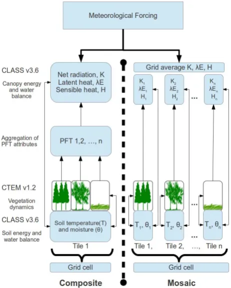
Fig. 1. Schematic representation of the composite and mosaic

ap-proaches for the coupling of CLASS v 3.6 and CTEM v 1.2 models in a stand-alone mode.

function of driving climate and atmospheric CO2

concentra-tion (CO2). Coupled LSSs and TEMs simulate fluxes of

wa-ter, energy and CO2at the atmosphere–land boundary.

Veg-etation in ESMs is commonly represented in terms of broad plant functional types (PFTs). Appropriate representation of these PFTs’ spatial distribution presents a challenge to mod-ellers, as the area of climate model grid cells is often on the order of 100 000 km2. On these large scales, the spatial distribution of terrestrial vegetation can be extremely hetero-geneous. For example, a grid cell with a land cover that is 20 % treed and 80 % herbaceous may represent a typical sa-vannah landscape with intermittent trees, or a closed-canopy forest surrounded by prairie grasslands. In reality, these two landscapes represent greatly different physical and hydrolog-ical environments for the plants growing within them. Earth system models thus need to adopt a strategy that can accu-rately capture the vegetation dynamics due to sub-grid scale variability without incurring excessive computational cost. In response to this requirement, the Earth system modelling community has adopted three main approaches to represent sub-grid scale vegetation variability within LSS frameworks, which are termed: (i) composite, (ii) mosaic, and (iii) mixed (following Li and Arora, 2012).

The composite approach (left column of Fig. 1) assumes that structural (as mentioned above) and physiological

at-tributes (e.g. stomatal conductance) of the PFTs present can be averaged across the grid cell (weighted by each PFT’s fractional coverage) (Verseghy, 1991; Verseghy et al., 1993; Sitch et al., 2003). These grid-averaged values are then used in water- and energy balance calculations to obtain a grid-averaged physical state of the land surface. Thus, each PFT is exposed to the same environmental variables, such as canopy temperature, soil moisture, soil temperature, and net radia-tion.

The mosaic representation of the land surface uses sepa-rate “tiles” for each PFT (Koster and Suarez, 1992a) (right column of Fig. 1). Each tile simulates the energy and wa-ter balance based upon the inwa-teractions of the structural and physiological characteristics of its PFT with the driving cli-mate, without regard to the conditions in the other tiles. As a result, the land surface state in each tile evolves indepen-dently with unique environmental variables with correspond-ing different simulated energy, water and CO2 fluxes. The

tiles fluxes are then grid-averaged prior to interaction with the lower boundary of the atmosphere.

The composite and mosaic approaches can be considered as the two extremes of the manner in which spatial variabil-ity of vegetation is represented. We term other approaches that lie in between the mosaic and composite as “mixed”. An example of the mixed approach uses the PFT vegetation attributes for calculations of the energy and water balance for each tile, but the soil moisture and temperature are grid-averaged at the end of each time step (Sellers et al., 1986; Dickinson et al., 1993; Oleson et al., 2010).

Different landscapes are better represented by one of the three approaches described above. Landscapes that are be-lieved to be better suited to a composite representation in-clude mixed deciduous broadleaf and evergreen needleleaf forests, as well as savannahs with sparse trees on grassland. The mosaic approach is suggested to better represent land-scapes with a clear distinction between PFTs such as non-overlapping cropland and closed-canopy forest. A mixed ap-proach is usually chosen to reduce computational cost, not specifically to better represent the land surface. Commonly, a model is run with a globally constant application of either composite or mosaic approaches, without consideration of the particular observed vegetation structure of an individual grid cell.

Their analysis was designed to generate the largest possible difference between the composite and mosaic approaches, as a form of sensitivity test, thus they used an idealized PFT fractional coverage of 50 % for each of the two dominant PFTs present at each location. Li and Arora (2012) reported that the primary energy fluxes were relatively insensitive to the vegetation representation, with less than 5 % difference between the two approaches. However, the carbon fluxes and pool sizes varied by as much as 46 % on a grid-averaged basis. Given that their simulations were intended to deter-mine the largest influence on a site level, it is difficult to pre-dict how important the vegetation configuration strategy is at a global scale, with realistic PFT fractional coverage, and under changing CO2, climate, and land use. Here, we expand

on the work of Li and Arora (2012) by studying the impact of the manner in which sub-grid scale variability of vegeta-tion is represented on the global terrestrial carbon balance. In addition, we investigate the model’s response to historical changes in (CO2), climate, and land cover when using the

composite and mosaic approaches.

2 Methods

2.1 Description of the CLASS and CTEM models

The CLASS-CTEM results presented here were generated from coupling of the CLASS (v. 3.6) (Verseghy, 2012) and CTEM (v. 1.2) models. Slightly older versions of both models are currently implemented in the second-generation Canadian Centre for Climate Modelling and Analysis Earth System Model (CanESM2) (Arora et al., 2011), but are used in an offline configuration here, driven with observation-based climate, to allow for simpler interpretation.

CLASS operates on a half-hourly time step driven with atmospheric forcing data (downwelling longwave and short-wave radiation, precipitation, air pressure, specific humidity, wind speed, and air temperature) and calculates the energy and water balances of the soil, snow, and vegetation canopy components. CLASS includes three soil layers of thickness: 0.10, 0.25, and up to 3.75 m (the depth of the third layer is dependent on the grid-cell soil depth to bedrock from Zobler, 1986). The temperature and liquid and frozen moisture con-tents are simulated for each soil layer. CLASS also simulates, when snow is present, the physical characteristics (mass, density, albedo, liquid water content, and temperature) of one snow layer of a prognostically determined depth. Within a single tile, surface flux calculations are performed on tile sub-regions of (as required): (i) bare soil, (ii) vegetation cov-ered ground, (iii) bare soil with snow cover, and (iv) veg-etation over snow. CLASS performs energy and water bal-ance calculations for four PFTs: needleleaf trees, broadleaf trees, crops, and grasses (short vegetation). Each PFT has prescribed structural attributes associated with it, such as leaf area index (LAI), plant height (roughness length), and

root-ing depth. However, when coupled to CTEM, these variables are dynamically modelled by CTEM and passed to CLASS.

CTEM simulates terrestrial ecosystem processes for nine PFTs that are directly related to the four CLASS PFTs. Needleleaf trees are separated into evergreen and decid-uous; broadleaf trees into evergreen, cold deciduous, and drought/dry deciduous; and crops and grasses are separated into C3and C4. In the version used here, CTEM simulates the

processes of photosynthesis, autotrophic and heterotrophic respiration, carbon allocation, phenology, turnover, and land use change.

CTEM operates on a daily time step (excluding the pho-tosynthesis, leaf respiration, and canopy conductance cal-culations which are performed on the CLASS time step). The photosynthesis and respiration (autotrophic and het-erotrophic) schemes of CTEM are described in Arora (2003). Positive net primary productivity (NPP) is allocated into three live carbon pools (roots, stems, and leaves). The pro-portional allocation to each of these pools is influenced by the leaf phenological, light and root water status of the plant (Arora and Boer, 2005). Turnover and mortality reduces the live carbon stock and contributes to two dead carbon pools (litter and soil organic matter). The disturbance (fire) module was not used in the simulations presented here.

The version of CTEM used here (v 1.2) differs from the previously published version of CTEM (v. 1.0 Arora, 2003; Arora and Boer, 2005) in: (i) its capability to perform both mosaic and composite simulations of the land surface under LUC; (ii) adjustments to photosynthesis parameters includ-ing maximum photosynthetic rate, Vc,max, (Rogers, 2013);

and (iii) adjustments to leaf maintenance and respiration rate parameters (see Table A1).

2.2 Carbon budget equations

The vertically integrated globally averaged carbon budget equation for the atmosphere can be represented as

dHA

dt =EF−FO−FL=(EF+ELUC)−FO−FLn, (1) whereHA is the global atmospheric carbon burden (Pg C),

FO andFLare the atmosphere–ocean and atmosphere–land

CO2 fluxes (Pg C yr−1), respectively, and EF is the

an-thropogenic fossil fuel emissions (Pg C yr−1). The global net atmosphere–land CO2flux (FL=FLn−ELUC), assumed

positive into the land, in CLASS-CTEM is the result of nat-ural CO2flux (FLn) and LUC emissions (ELUC) associated

with changes in land cover (with the convention of positive into the atmosphere). The curly braces around the LUC term symbolize the LUC term to be made up of many different LUC processes. The globally averaged land carbon budget is represented as

FL=

dHL

dt = dHV

dt + dHS

dt

where HL=HV+HS, represents the global land carbon

mass, which includes the live vegetation biomass,HV, and

the dead carbon in the soil and litter pools,HS. GPP is gross

primary productivity, which yields NPP after autotrophic res-piration (RA) is accounted for. RH is heterotrophic

respi-ration. When land cover is not changing, the term ELUC

is zero andFL=FLnrepresents net ecosystem productivity

(NEP). In the presence of LUC and other disturbances (if any), the termFLrepresents net biome productivity (NBP);

for more discussion on the difference between NEP and NBP see (Chapin et al., 2006). Integrating Eq. (2) gives the change in total land carbon with respect to the cumulative land– atmosphere CO2flux (F˜L):

˜

FL=

Rt

toFLdt=1HL=1HV+1HS

=Rt

toNPP dt−

Rt toRHdt−

Rt toELUCdt

˜

FL= ˜FLn− ˜ELUC, (3) where the termsF˜LnandE˜LUCrepresent cumulative NEP

and cumulative LUC emissions, respectively.

2.3 Land use change

In CLASS-CTEM, LUC emissions are treated in a fully inter-active manner, where an increase in crop area occurs through deforestation/clearing of natural vegetation and a reduction in theHV of natural woody or herbaceous vegetation (see

Arora and Boer, 2010). When crop area expands into the nat-ural vegetated areas of the grid cell, as determined by the HYDE v 3.1 data set (Hurtt et al., 2011), the biomass re-moved,L(kg cm−2), is divided into three components such thatL=LA+LS+LD. The first component, LA, is

com-busted during clearing, or used immediately for fuel wood, and emitted to the atmosphere as CO2; the second

compo-nent,LS, is assigned to pulp and paper products, or left in

place as slash; while the final component,LD, is used for

durable wood products. The fraction ofL for each compo-nent (LA,LSorLD) depends on whether the PFT is woody or

herbaceous and the aboveground vegetation biomass density (see Table 1 in Arora and Boer, 2010). To approximate the lifetimes of theLS andLD components, these components

are allocated to the litter and soil carbon pools, respectively. As a result the carbon that is removed from live vegetation is emitted to the atmosphere either immediately (LA), or with

some delay depending on the decomposition rate of the litter or soil C pools. Crop PFT biomass is annually transferred to the soil litter pool (LS) when the crop has matured

(signi-fied by leaf area index reaching 3.5 m2m−2_forC

3crops and

4.5 m2m−2 _{for C}

4 crops). This approach allows LUC

im-pacts to influence all aspects of the terrestrial carbon budget including vegetation, litter and soil carbon pools and fluxes. The emissions of carbon due to LUC are evident in theELUC

term as direct CO2emissions but also in increased litter and

soil C pool sizes, and subsequently, fluxes. When crop area fraction in a grid cell decreases, the fraction under natural vegetation is increased, which reduces the biomass density, causing the vegetation to uptake more carbon until it reaches

Fig. 2. Comparison of simulated zonally averaged (a) GPP, (b)

veg-etation biomass, and (c) soil carbon with observation-based esti-mates. The CLASS-CTEM results from the simulations using com-posite and mosaic configurations are averaged over the 1996–2005 period and are from the Climate+CO2+LUC simulation.

a new equilibrium, creating the land-use-related carbon sink that is, for example, associated with abandonment of crop-lands. In practice, ELUC is not straightforward to diagnose

and at least two simulations are required. As in McGuire et al. (2001) and Arora and Boer (2010), for example, we di-agnoseELUCas the difference in atmosphere–land CO2flux

from simulations with and without LUC.

2.4 Model inputs

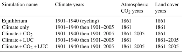
All CLASS-CTEM simulations were performed at the Gaus-sian 96×48 grid cell resolution (approximately 3.75◦×

Table 1. CLASS-CTEM simulations performed for the composite and mosaic configurations. For the transient simulations (last four listed

below), the simulation years of 1861–1900 were forced with climate from 1901 to 1940; simulation years 1901–2005 were forced with climate years from 1901 to 2005.

Simulation name Climate years Atmospheric Land cover CO₂years years

Equilibrium 1901–1940 (cycling) 1861 1861 Climate only 1901–1940 then 1901–2005 1861 1861 Climate + CO2 1901–1940 then 1901–2005 1861–2005 1861

Climate + LUC 1901–1940 then 1901–2005 1861 1861–2005 Climate + CO2+ LUC 1901–1940 then 1901–2005 1861–2005 1861–2005

Longwave radiation was uniformly distributed over the 6 h period. Surface temperature, wind speed, surface pressure, and specific humidity were linearly interpolated. The total 6 h precipitation amount was used to determine the number of wet half-hour time steps following Arora (1997). The total 6 h amount was then distributed amongst the wet time steps. Soil texture information was adapted from Zobler (1986) with soil texture within each grid cell kept the same for both composite and mosaic configurations. For the histori-cal 1850–2005 period, the (CO2) is based on phase 5 of the

Coupled Model Intercomparison Project (CMIP5) data set (Meinshausen et al., 2011). The changes in fractional cov-erage of non-crop PFTs are inferred based on the changes in crop area following the HYDE v 3.1 data set (Hurtt et al., 2011) using the linear interpolation approach of Arora and Boer (2010). The resulting transient land cover for the period 1850–2005 has also been used in CanESM2’s simulations for CMIP5 (Arora et al., 2011).

2.5 Simulations

Results from five simulations are presented for both the mo-saic and composite approaches (Table 1). The pre-industrial equilibrium spin-ups, corresponding to the year 1861, form the starting point for each of the four transient historical runs (1861–2005), which were driven with different combi-nations of CO2, climate and LUC forcings. These include:

(i) evolving climate with fixed 1861 land cover and (CO2)

(“Climate only”), (ii) evolving climate and CO2 with fixed

1861 land cover (“Climate+CO2”), (iii) evolving climate

and land cover with fixed 1861 (CO2) (“Climate+LUC”),

and (iv) evolving climate, (CO2), and land cover

(“Cli-mate+CO2+LUC”). Since the CRU-NCEP climate data

does not extend back past 1901, for the period 1861–1900 we use the climate of 1901–1940. We also do not extend past 2005 as that is the last year in the HYDE v. 3 data set as used in the CMIP5 simulations. For most of the results presented here, we limit our analysis to the 1959–2005 period for ease of comparison with the results of other dynamic vegetation models and the estimated terrestrial C land sink as summa-rized in Le Quéré et al. (2013).

The pre-industrial equilibrium run used a constant, glob-ally uniform (CO2) of 286.37 ppm corresponding to observed

atmospheric concentration in the year 1861 (Meinshausen et al., 2011) with PFT fractional coverage corresponding to the year 1861 and climate from 1901 to 1940 cycled over repeatedly until model pools reached equilibrium (Ta-ble 1). Equilibrium is assumed to have been attained when net ecosystem productivity,FLn, varies less than 0.001 % of

NPP averaged across the final 40 yr of the simulation. Com-posite and mosaic simulations were spun up separately.

3 Results

3.1 Comparison to observationally based data sets

The pre-industrial equilibrium simulations global totals for primary model outputs are listed in Table 2. Both the com-posite and mosaic approaches simulate global totals of GPP, NPP, soil respiration, vegetation biomass, litter mass, and soil carbon in line with observation-based estimates and previ-ous modelling studies of the pre-industrial period (Table 2). For these global sums, the difference between the composite vs. mosaic approach is minor (maximum 4.6 %). Overall, the composite approach yields higher productivity and respira-tory fluxes, and higher vegetation and soil carbon pools, than the mosaic approach.

Zonally, CLASS-CTEM reproduces reasonable patterns of GPP, vegetation biomass and soil carbon as compared to observation-based data sets for contemporary condi-tions (Fig. 2). While the CLASS-CTEM results (“Cli-mate+CO2+LUC”) in Sect. 2 include the influence of

CLASS-CTEM simulates slightly higher values at the equa-tor and below about 35◦_{S than Beer et al. (2010), but slightly}

lower values for latitudes>45◦_{N and around 15}◦_{N. The}

composite and mosaic CLASS-CTEM zonal GPP shows only small differences around 10–30◦N and around 20– 40◦S, with a higher GPP simulated when using the compos-ite approach.

For zonally averaged vegetation biomass (Fig. 2b), CLASS-CTEM simulates an equatorial peak in vegetation biomass slightly higher than the Ruesch and Holly (2008) data set for both approaches. This data set is based upon re-motely sensed vegetation cover (Global Land Cover 2000 Project, GLC2000) and IPCC methods for estimating car-bon stocks at the national level. For latitudes>30◦N and <30◦S, CLASS-CTEM simulates a higher mean vegetation biomass than Ruesch and Holly (2008) with a prominent peak around 45◦_{S. The mosaic and composite approaches}

differ little in zonal mean vegetation biomass except for small differences around 10–30◦N where the composite ap-proach has a noticeably higher value. The methods employed to create the Ruesch and Holly (2008) data set are not di-rectly linked to ground-based measures of carbon stocks and have also not been validated with field data. The data set may underestimate vegetation biomass at high latitudes. For ex-ample, its vegetation biomass values are less than half that of inventory based estimates for British Columbia, Canada (Peng et al., 2013).

The CLASS-CTEM mosaic and composite approaches’ zonally averaged soil carbon is compared to the Harmonized World Soils Dataset (HWSD) (FAO, 2012) in Fig. 2c. The HWSD is more reliable for southern and Eastern Africa, Latin America and the Caribbean, and central and eastern Europe. It is considered less reliable for North America, Aus-tralia, areas of West Africa and South Asia (FAO, 2012). While the zonal distribution of simulated soil carbon is broadly similar to observation-based HWSD estimates, some differences remain. Between 45–70◦N, CLASS-CTEM sim-ulates appreciably less soil carbon than the HWSD, with val-ues around 15◦N, and below 50◦S also lower (below 50◦S has little landmass thus the large value in the HWSD is likely the result of high values in relatively few grid cells). Some of the difference between CLASS-CTEM and HWSD is due to the fact that peatlands, which contain high amounts of organic carbon, are not presently simulated by CLASS-CTEM. This is especially noticeable in the region of 45– 70◦_{N. CLASS-CTEM simulates appreciably more soil}

car-bon around 30–50◦_{N and in most of the Southern}

Hemi-sphere.

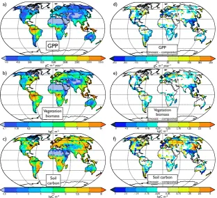
3.2 Spatial differences between the approaches

Figure 3a–c shows the spatial distribution of simulated GPP, vegetation biomass and soil C mass from the pre-industrial equilibrium simulation when using the mosaic approach. The corresponding spatial differences between the composite and

mosaic approaches are shown in Fig. 3d–f. The major re-gions of difference for vegetation biomass and GPP, which can be>30 %, include Southeast Asia, the Pampas region in Argentina, the west coast of North America, southeast US, northern mainland Europe, and Mexico (Fig. 3d and e). In each of those regions, the composite simulation calculates higher GPP and vegetation biomass. The mosaic approach yields higher GPP and vegetation biomass for some regions, such as eastern Canada, China, the central US, and Patag-onia, however the magnitude of the difference is smaller than for the regions where the composite approach simu-lates larger values. The simulated soil carbon mass differ-ences between the mosaic and composite runs (Fig. 3f) fol-low a similar pattern to the differences in vegetation biomass with Southeast Asia, the Pampas of Argentina, the west coast of North America, northwest mainland Europe, and south-east Australia, simulated to have higher soil carbon mass in the simulation using the composite approach. Some other re-gions show contrasting patterns between vegetation biomass and soil carbon, including the southeast US, the Chilean coast, the Baltics, and western Russia, although the differ-ences are relatively small.

3.3 Transient historical simulations

Four simulations were performed to investigate the effect of using the composite versus mosaic approach on the histor-ical terrestrial carbon budget. The simulations were driven with different combinations of CO2, climate and LUC

forc-ings (as described in Sect. 2.5 and Table 1): (i) Climate only, (ii) Climate + CO2, (iii) Climate + LUC, and (iv)

Cli-mate + LUC + CO2.

In Fig. 4a, simulatedF˜L from the Climate+CO2

simu-lation (using both the composite and mosaic approaches) is compared to an observation-based estimate and simulations from eight other TEMs/DGVMs (as presented in Le Quéré et al., 2013). The Climate + CO2 simulation does not

in-clude land use change, thus F˜L= ˜FLn, which essentially

represents cumulative NEP. F˜Ln is also referred to as the

residual terrestrial C sink, whose value can be determined as the residual of other observation-based terms in Eq. (1). The observation-based estimate ofF˜Lnfrom Le Quéré et al.

(2013) in Fig. 4a is their estimate of the residual terrestrial C sink after accounting for fossil fuel and LUC emissions, change in atmospheric C burden and the ocean C sink. This does not include gross land C sinks directly resulting from LUC (e.g. regrowth of vegetation), but does include the in-fluence of CO2 fertilization, nitrogen deposition, and other

climate change effects such as changes to growing season length. SimulatedF˜Ln, over the 1959–2005 period, does not

a) d)

b) e)

c) f)

GPP

Vegetation biomass

Soil carbon

Soil carbon (mosaic - composite)

Vegetation biomass (mosaic - composite)

GPP (mosaic - composite)

gC m-2 _year-1

kgC m-2 _{kgC m}-2

kgC m-2 _{kgC m}-2

gC m-2 _year-1

Fig. 3. Pre-industrial equilibrium CLASS-CTEM results using the mosaic approach for (a) GPP, (b) vegetation biomass, and (c) soil carbon

mass. The difference between the mosaic and composite approach is shown in the right-hand column for (d) GPP, (e) vegetation biomass, and

(f) soil carbon mass. Positive values indicate that the values from the mosaic approach are larger; negative values indicate that the composite

approach yields larger values.

Table 2. Results from the pre-industrial equilibrium simulations using the composite and mosaic model configurations. Values are a 40 yr

average at the end of model spin-up. The spin-up cycled over climate years 1901–1940 with year 1861 atmospheric (CO2) and land cover.

Variable Model outputs Preindustrial values from Other modern

Composite Mosaic Difference (%) modelling studies estimate

Gross primary productivity (Pg C yr−1_{) 121.8 117.3 3.8 134.0 (Gerber et al., 2004) ca. 125 (Zhao et al., 2006)}a_,

123±8b(Beer et al., 2010) Net primary productivity (Pg C yr−1) 61.0 58.5 4.3 64.0 (Sitch et al., 2003), 50–70

(Friedlingstein et al. , 2006)

59.9 (Ajtay et al., 1979), 62.6 (Saugier et al., 2001), 56.6 (Running et al., 2004) Litter respiration (Pg C yr−1) 41.8 40.1 4.2

Soil carbon respiration (Pg C yr−1) 19.2 18.4 4.3

Soil respiration (litter+soil C) (Pg C yr−1) 61.0 58.5 4.1 68±4 (Raich and Schlesinger, 1992),

76.5 (Raich and Potter, 1995)

Vegetation biomass (Pg C) 530 507 4.6 932 (Sitch et al., 2003) 446 (Ruesch and Holly, 2008)c

Litter mass (Pg C) 97 94 2.9 171 (Sitch et al., 2003) 90 (Ajtay et al., 1979) Soil carbon mass (Pg C) 1409 1404 0.03 1670 (Sitch et al., 2003) 1400–1600 (Schlesinger, 1977),

1395 (Post et al., 1982), 1348 (FAO, 2012)c

a_{MODIS-derived LAI driven with NCEP reanalysis.}b_{Estimate for modern-day, which includes the effects of elevated CO}

2and anthropogenic land use.cInterpolated

to T47 resolution and using the same land mask as CLASS-CTEM.

Introducing changes in land cover imply that the term ELUC is not zero and the cumulative atmosphere–land CO2

flux is reduced (F˜L= ˜FLn− ˜ELUC) to yield the

cumula-tive NBP. Note that our definition of NBP, in the context of CLASS-CTEM, does not include the effect of

distur-bance agents such as fire, insects, management-climate in-teractions, and nitrogen dynamics. Figure 4b shows the cu-mulative deforested biomass in the Climate+LUC+CO2

Fig. 4. CLASS-CTEM results from the transient simulations over

the 1959–2005 period using the composite and mosaic approaches.

(a) The simulated cumulative atmosphere–land CO2 flux (F˜Ln)

from the Climate+CO2simulation in comparison with other

ter-restrial vegetation model estimates and the estimated residual land sink from Le Quéré et al. (2013). None of the model results in-clude LUC and all simulations/estimates account for changing cli-mate and atmospheric (CO₂). (b) Deforested biomass from the Cli-mate+CO2+LUC simulation alongside the bookkeeping-based

estimate of LUC emissions from Houghton et al. (2012). (c) Results from the four different transient simulations using different combi-nations of climate, (CO2), and LUC forcings. The model setup for

each run is described in Sect. 2.5 and Table 1. Negative and positive

˜

FLandF˜Lnvalues indicate net carbon release from the land surface

to the atmosphere and uptake by the land surface, respectively.

is somewhat higher in the composite approach (22.4 Pg C) than when using the mosaic approach (17.8 Pg C) because of its higher vegetation biomass. However, these values of de-forested biomass are much lower than the Houghton et al. (2012) estimate of LUC emissions (68.8 Pg C) over the same period (calculated from original data available at http://cdiac. ornl.gov/trends/landuse/houghton/houghton.html). The LUC emissions from Houghton et al. (2012) are based on a

“book-keeping” approach where changes in cropland and pasture area, wood harvesting and logging, and shifting cultiva-tion are accounted for via transfer to pools with prescribed turnover rates. Our LUC parametrization does not take into account wood harvesting or logging, shifting cultivation and conversion to pasture.

Figure 4c compares cumulative atmosphere–land CO2flux

˜

FL from all four simulations when using both the

mo-saic and composite approaches. Over the 1959–2005 pe-riod, the Climate only simulation shows no strong net emis-sion, or uptake, of carbon by the land surface when us-ing the mosaic approach (0.0 Pg C) and a slight carbon uptake by the land surface when the composite approach is used (4.1 Pg C). The Climate+LUC simulations give a net land C source with mosaic and composite cumula-tive NBP values of 7.6 Pg C and 10.2 Pg C, respeccumula-tively. Cli-mate+CO2 simulations show a large terrestrial carbon

up-take of 96.3 Pg C and 101.3 Pg C for mosaic and composite approaches, respectively, as also seen in Fig. 4a. Finally, the Climate+LUC+CO2simulation reduces the estimated

ter-restrial C sink slightly to 95.1 Pg C (1 % reduction compared to the Climate+CO2simulation) when using the mosaic

ap-proach, but a much stronger reduction is seen in the compos-ite approach (79.9 Pg C; 21 % reduction compared to the Cli-mate+CO2simulation) at the end of the 1959–2005 period.

Overall, the difference between the composite and mosaic approaches, for global carbon uptake, is most pronounced for the Climate+CO2+LUC simulation. Diagnosing

cumula-tive LUC emissions,E˜LUC, as the difference between

cumu-lative atmosphere–land CO2flux between the Climate+CO2

and Climate+CO2+LUC simulations, in a manner similar

to McGuire et al. (2001) and Arora and Boer (2010), we ob-tainE˜LUCas 21.4 Pg C and 1.2 Pg C for the composite and

mosaic approaches, respectively.

Geographical distributions of the difference in atmosphere–land CO2 flux (FL) averaged over the period

1959–2005 between the mosaic and composite approaches are shown in Fig. 5 from the Climate+CO2 (panel a)

and Climate+CO2+LUC (panel b) simulations. For the

Climate+CO2simulation (Fig. 5a) the difference between

the mosaic and composite approaches is greatest in the Pampas region of Argentina, Southeast Asia and southern China, northern India, Tanzania, and parts of Mexico where the composite approach simulates a larger C sink. Although there are some regions (including the American Midwest and parts of Scandinavia and western Russia) where the mosaic approach yields a larger C sink, in the Climate+CO2

a) b)

Fig. 5. Difference in the simulated atmosphere–land CO2 flux averaged over the 1959–2005 period between the mosaic and composite

approaches for (a) the Climate+CO₂run and (b) the Climate+CO₂+LUC run. Negative values indicate the atmosphere–land CO₂flux is greater when using the composite approach; positive values indicate the atmosphere–land CO2flux is greater for the mosaic approach.

Fig. 6. Heterogeneity index for 1861 land cover based on the HYDE

v 3.1 crop data set. This index is defined in Sect. 4.

Fig. 7. Mean annual relative change in the crop cover,R¯C, due

to historical anthropogenic land use (1959–2005). This measure of land use change is defined in Sect. 4.

4 Discussion

CLASS-CTEM produces estimates of GPP, NPP, soil respi-ration, vegetation biomass, and litter and soil carbon mass that compare reasonably well with observational estimates

and previous modelling studies of the pre-industrial period (Fig. 2 and Table 2) for both mosaic and composite configu-rations. The importance of the composite or mosaic approach in an equilibrium simulation on a global scale is minor, with the difference consistently<5 % for several model variables. However, the spatial differences are much greater and appear to be consistent across different model variables including GPP, vegetation biomass and soil C mass (Fig. 3). The differ-ences between the mosaic and composite approaches are re-lated to the representation of sub-grid scale variability of veg-etation and the consequent manner in which grid-averaged energy and water balances evolve, leading to differences in net radiation absorbed by vegetation, soil temperature and moisture, etc., as illustrated in Li and Arora (2012). To aid interpretation of the differences between simulations using the mosaic and composite approaches, we derive a hetero-geneity (H) index as follows:

H=1−

1

N−1

N

P

i=1

(fi− ¯f )2

¯

f , (4)

a) b)

c) d)

1860 1880 1900 1920 1940 1960 1980 2000

0

20

40

60

80

100

Percent of g

rid cell

Needleleaf evergreen Needleleaf deciduous Broadleaf evergreen

Broadleaf cold deciduous Broadleaf drought/dry deciduous C3 crop

C4 crop C3 grass C4 grass

Bareground

gC m

2 yr

1

350 400 450 500 550 600

kgC m

2

1.0 1.5 2.0 2.5

gC m yr

2 –1

0 10 20 30 40

Year

gC m

2

1860 1880 1900 1920 1940 1960 1980 2000 0

Year

kgC m

2

1860 1880 1900 1920 1940 1960 1980 2000 11.5

12.0 12.5 13.0 13.5 14.0 14.5

e) f)

Fig. 8. CLASS-CTEM results for the mosaic and composite approaches for a grid cell at 50.10◦N and 46.88◦E (near Volgograd, Russia) from

the Climate+CO2+LUC simulation. (a) Specified changes in PFT fractional cover, (b) vegetation biomass, (c) net primary productivity

(NPP), (d) total deforested biomass as a result of LUC, (e) soil C pool, and (f) total cumulative NBP (F˜L). The model outputs have a 10 yr

running mean (thick lines) applied to the annual values (thin lines)

H index is not a prescriptive measure as it does not include information about a grid cell’s climate and soil conditions. It is intended to highlight areas that could be expected to have greater differences between the composite and mosaic configurations due to PFT spatial representation. The global distribution of theH index (based on 1861 land cover, used here with crop fraction based on the HYDE v 3.1 data set) is shown in Fig. 6. Areas of highHindex include parts of Mex-ico, Europe, China, India, eastern Australia, and the eastern US. Areas of lowH index include arid regions, such as cen-tral Auscen-tralia; tropical regions, such as the Amazon; and the high north. Areas of lowH index are thus regions with veg-etation biomass spread across very few PFTs.

Comparing theHindex (Fig. 6) to spatial differences be-tween composite and mosaic simulations for the equilibrium simulation (Fig. 3) demonstrates a reasonable linkage. Ar-eas of high H index generally have higher GPP, vegeta-tion biomass and soil carbon mass when the composite ap-proach is used. Regions with moderateH index values are

not strongly biased towards either approach. Areas of lowH are generally similar in simulations using the composite and mosaic approaches, as expected. The differences between the model configurations evident in Fig. 3 are related to differ-ences in the energy and water balances calculations in the two approaches, as noted by Li and Arora (2012). Li and Arora (2012) observed differences in net radiation flux (due to albedo differences); latent and sensible heat flux; and soil moisture and temperature between the composite and mo-saic configurations, at their selected sites, when driven with identical climate. Net radiation and soil moisture directly in-fluence photosynthesis and simulated canopy and soil tem-peratures influence respiratory fluxes.

Across the historical period (1959–2005) in the Cli-mate+CO2 simulation, CLASS-CTEM simulates a global

Fig. 9. Global response to LUC for the composite and mosaic

ap-proaches over the 1959–2005 period. The difference between the simulations with LUC (Climate + LUC + CO₂) and without LUC (Climate + CO2) for the cumulative change in the soil and litter

(1HS) (left panel) and vegetation pools (1HS) (centre panel) are

defined following Eq. (9). The cumulative LUC emissions (E˜LUC)

for the composite and mosaic approaches is shown in the right panel as the additive result of the left and centre panel.

but can be large for different regions. The areas of largest dis-agreement for the estimated terrestrial C sink (without LUC effects) between the composite and mosaic simulations are generally regions of highHindex, with a few notable excep-tions such as areas in the US Prairies (compare Figs. 5a and 6).

Incorporation of LUC has a marked impact on the differ-ence in the estimated global terrestrial C sink (cumulative NBP; Fig. 4c) between the simulations using the mosaic and composite configurations. Our simulated deforested biomass across both configurations is lower than the bookkeeping es-timate of Houghton et al. (2012) since we take into account only the changes in crop area, i.e. the effect of increasing pasture area over the historical period is not considered, and we do not account for wood harvesting and logging, shift-ing cultivation, and urbanization which is also not consid-ered by Houghton et al. (2012). Land use change emissions are extremely difficult to quantify, with at least a ±50 % uncertainty (Houghton, 2003), and LUC is represented in TEMs and DGVMs using a range of parametrizations (e.g. see Brovkin et al., 2013).

LUC causes the estimated terrestrial C sink to drop by 21.4 Pg C when using the composite approach, as would be generally expected since LUC releases carbon from burning and decomposition of the deforested biomass. In the mosaic configuration, however, LUC causes the terrestrial sink to drop by only 1.2 Pg C (Fig. 4c; compare Climate+CO2vs.

Climate+CO2+ LUC), yielding a 16 % difference in the

es-timated global terrestrial sink, over the 1959–2005 period, between the two approaches. The larger effect of LUC on the composite configuration’s cumulative NBP, over the mosaic, appears to be widespread globally (Fig. 5b vs. 5a).

The LUC scheme in CLASS-CTEM removes natural veg-etation when crop area increases. When LUC occurs, the amount of C that is burned or transferred to the litter and soil C pools depends on the vegetation biomass of the PFT that occupies that fraction of grid cell that is encroached upon at the time of LUC. In CLASS-CTEM, crops generally have a higher maximum photosynthetic rate than the natural vege-tation they replace. However, crop productivity also depends on whether the mosaic or composite configuration is used. To interpret the differences between the mosaic and composite approaches, in the simulation with LUC, we define an ad-ditional measure that quantifies changes in crop fraction in a grid cell. The mean annual relative change in crop fraction,

¯

RC, is calculated as

¯

RC=

T

X

t=2

|fc(t )−fc(t−1)|

T−1 ×100 %, (5)

wherefc(t )is the fractional crop area for a grid cell at time

t and T is 47 yr, i.e. the period 1959–2005. TheR¯C over

the 1959–2005 period is shown in Fig. 7. The major ar-eas of LUC include the US Midwest and prairie region of Canada, eastern Europe, western Russia, and parts of north-ern India, China, southeast Australia and Argentina. While theH index is arguably sufficient for interpreting the differ-ences in the simulations with mosaic and composite configu-rations evident in Fig. 5a (Climate+CO2), i.e. in simulations

without LUC, the contribution of both heterogeneity (Fig. 6) and LUC (Fig. 7) cause the differences inF˜L between the

composite and mosaic configurations visible in Fig. 5b (Cli-mate+CO2+LUC). In general, areas of highHindex have

greater visible differences between the mosaic and compos-ite approaches, and these are then exaggerated by LUC pro-cesses, since the effect of LUC is influenced by the manner in which vegetation is represented.

To illustrate how the effect of LUC depends on represen-tation of vegerepresen-tation (using the composite or the mosaic ap-proach) we show results from a grid cell that is representa-tive of regions with highHindex and high LUC (Fig. 8) over the simulated historical period (1861–2005). Grid cells with a highHindex demonstrate larger differences between mo-saic and composite treatments, as already discussed, and ar-eas of high LUC accentuates differences between the model approaches. In the grid cell chosen for this purpose (50.10◦N and 46.88◦_{E, near Volgograd, Russia), there is a large LUC,}

as evident in a doubling of C3crop fraction and a resulting

re-duction in the tree fraction, between 1861 and 2005 as seen in Fig. 8a. For this grid cell, the composite approach simulates a larger vegetation biomass in 1860 in the pre-industrial equi-librium simulation (Fig. 8b) due to a higher grid-averaged NPP (Fig. 8c). As the C3 crop fraction expands, the

the live vegetation pools differs between the composite and mosaic simulations (Fig. 8d), since the amount of biomass removed depends on the amount that is present, but over-all with the same pattern. That is, despite the same changes in fractional coverage of PFTs between the approaches, the amount of natural vegetation deforested differs. Since the deforested biomass is larger in the composite approach, over the historical period, it simulates a steeper decline in grid-averaged vegetation biomass (Fig. 8b). The soil C pools are initially smaller for the composite configuration (Fig. 8e) due to higher soil temperatures (not shown) despite higher litter inputs associated with higher initial productivity (Fig. 8c) in the composite compared to the mosaic approach. As carbon is transferred to the soil C pool by LUC, the two configu-rations diverge further. Soil C mass decreases in the com-posite approach and increases in the mosaic approach. The decline in soil C mass in the composite approach is due to the faster rate of shrinking vegetation biomass (Fig. 8b) and diminishing amounts of biomass transferred, as well as warmer soils in the composite approach promoting faster de-composition. As crop area expands, the grid-averaged NPP in the mosaic configuration approaches that of the composite (Fig. 8c) due to a faster rate of increase of crop productivity (not shown). Recall that in the mosaic configuration crops are grown in their individual tile, while in the composite ap-proach they share the same physical land surface climate, in-cluding soil moisture, as other PFTs. The net result is that the trajectory of the cumulative atmosphere–land CO2 flux

(F˜L) differs greatly between composite and mosaic for this

grid cell (Fig. 8f). Over the 1861–2005 period, the compos-ite approach yields a net source of C, while the mosaic ap-proach simulates the grid cell to be a C sink. The differences in simulated energy and water balances between the two ap-proaches act in a manner such that in the mosaic approach, the increasing productivity associated with increasing crop area overcomes the resulting emissions from burning and de-composition of deforested biomass. The different responses of grid-averaged carbon balance in this grid cell illustrate how the net effect of global LUC can be quite different for the two approaches.

On a global scale, similar behaviour is observed across the 1959–2005 period as has been described for the example above. Cumulative LUC emissions (E˜LUC)

can be represented by rearranging Eqs. 3 and 2 in terms of changes in the vegetation biomass (1HV) and

dead carbon (soil and litter, 1HS) pools for the

sim-ulations with LUC (CO2+Climate+LUC) and without

(CO2+Climate). The cumulative atmosphere–land CO2flux

for the CO2+Climate simulation, i.e. the NEP, is written as

˜

FLn=1HV_CO2+Climate+1HS_CO2+Climate. (6)

The cumulative atmosphere–land CO2 flux for the

CO2+Climate+LUC simulation, i.e. the NBP, is written as

˜

FL=1HV_CO2+Climate+LUC+1HS_CO2+Climate+LUC, (7)

with_E˜

LUC= ˜FLn− ˜FLand rearranging Eqs. 6 and 7 we can

solve forE˜LUCas

˜

ELUC=(1HV_CO2+Climate−1HV_CO2+Climate+LUC) (8)

+(1HS_CO2+Climate−1HS_CO2+Climate+LUC),

which shows that the E˜LUC term consists of differences in

live vegetation and dead litter and soil carbon pools from simulations with and without LUC. Figure 9 shows E˜LUC

and its two components from the simulations using com-posite and mosaic approaches as a function of time for the period 1959–2005. The difference in the dead C pools for simulations with and without LUC (1HS_CO2+Climate −

1HS_CO2+Climate+LUC) shows a divergent response between the

composite and mosaic approaches. The composite approach loses soil and litter carbon under LUC, while the mosaic approach gains carbon (left panel of Fig. 9). This response is similar to that seen in the Russian grid cell discussed above. As the usual configuration of CLASS-CTEM uses the composite approach, this behaviour was not apparent un-til comparison was possible between the two approaches. The response of vegetation biomass to LUC (1HV_CO2+Climate

– 1HV_CO2+Climate+LUC) is more similar between the two

ap-proaches with the expected loss of vegetation biomass due to LUC. The composite configuration loses more vegetation carbon than the mosaic configuration due to its higher pre-industrial vegetation biomass (middle panel of Fig. 9). Taken together for an estimate of the cumulative LUC emissions over the 1959–2005 period (E˜LUC), following Eq. (9), the

gains in soil carbon in the mosaic approach negate much of the losses in vegetation biomass to give a small_E˜

LUCwhile

the composite approach shows higher E˜LUC due to source

contributions from both the dead and live carbon pools (right panel of Fig. 9).

The strong influence of the model vegetation spatial con-figuration has implications for model estimates of carbon emissions due to LUC. Estimates of the total LUC emis-sions range from 72 Pg C to 115.2 Pg C across the 1920– 1999 period (Houghton et al., 2012). The CLASS-CTEM LUC parametrization gives a global LUC emissions esti-mate that is on the low end of other models. Arora and Boer (2010) estimate 73.6 Pg C across the same time pe-riod from Table 1 in Houghton et al. (2012) using CLASS v. 2.7 with CTEM v. 1.0 in a composite configuration imple-mented in the first-generation Canadian Earth System Model (CanESM1) (Arora et al., 2009).

Table A1. CTEM parameter values updated in v 1.2 over v 1.0 (Arora and Boer, 2005) of maximum rate of carboxylation by the enzyme

Rubisco,Vc, max(Rogers, 2013), leaf maintenance respiration, and litter and soil carbon respiration rate.

PFT Vc, max Leaf maintenance Litter respiration Soil carbon

(10−6mol CO2) respiration rate at 15◦C respiration rate

m−2s−1 coefficient (kg C kg−1C yr−1) at 15◦C (unitless) (kg C kg−1C yr−1) Needle-leaved evergreen 35 0.015 0.4453 0.0260 Needle-leaved deciduous 40 0.017 0.5986 0.0260 Broadleaf evergreen 51 0.020 0.6339 0.0208 Broadleaf cold deciduous 67 0.015 0.7576 0.0208 Broadleaf drought/dry deciduous 40 0.015 0.6957 0.0208

C₃crop 55 0.015 0.6000 0.0350

C4crop 40 0.025 0.6000 0.0350

C₃grass 75 0.013 0.5260 0.0125

C4grass 15 0.025 0.5260 0.0125

model architecture can have a significant influence on mod-elled LUC emissions.

5 Conclusions

Dynamic vegetation models must represent the sub-grid het-erogeneity of terrestrial vegetation in a manner that is com-putationally efficient and best captures vegetation dynamics. The two possible extremes of the manner in which vegetation sub-grid spatial variability may be represented are the com-posite and mosaic approaches (Fig. 1). The impact of which model approach to use to best represent PFT spatial het-erogeneity has not been adequately investigated previously. Here, we have used global simulations of the terrestrial car-bon budget over the historical period to illustrate the effect of using the composite versus the mosaic approach.

In our equilibrium spin-up simulations using CLASS-CTEM, in either the composite or mosaic configurations, we see no large differences in the global sums of model variables like vegetation biomass, GPP, NPP, soil C and litter mass be-tween the two approaches (<5 %). However, spatially, the differences between the two approaches can be large for these model variables (>30 %). These differences are most apparent in regions with high heterogeneity of land cover (with regard to the number of PFTs) where the mosaic and composite representations are less comparable. In transient simulations, the mosaic and composite approaches respond differently to changing climate and CO2. The difference in

cumulative atmosphere–land CO2 flux is 5 Pg C, or around

5 %, over the 1959–2005 period in Climate+CO2

simula-tions. When LUC is accounted for, the difference between the cumulative atmosphere–land CO2flux in the simulations

using the composite and mosaic configuration increases to 15.2 Pg C (or around 16 %) and spatial differences increase further. The diagnosed LUC emissions, calculated as the difference between cumulative atmosphere–land CO2 flux

from simulations with and without LUC, are 21.4 Pg C and 1.2 Pg C for the composite and mosaic approaches, respec-tively. These estimates are much lower than Houghton et al. (2012) since we do not account for changes in pasture area, wood harvesting, or shifting cultivation. CLASS-CTEM also treats crop PFTs explicitly, rather than using grass PFTs in place of crops as is common among most ESMs (Brovkin et al., 2013). In CLASS-CTEM, the high maximum photo-synthesis rate of crops contributes to the higher rate of NPP increase as croplands expand and as CO2increases and this

acts to lower estimated LUC emissions in the mosaic ap-proach. Irrespective of comparison with the Houghton et al. (2012) estimate, our results show that the difference between the two approaches of representing sub-grid heterogeneity of vegetation is largest when LUC is accounted for in conjunc-tion with increasing CO2and changing climate. The

CLASS-CTEM LUC scheme is sensitive to the vegetation productiv-ity and biomass in a grid cell. Since the energy and water balances evolve differently in composite vs. mosaic config-uration (as noted in Li and Arora, 2012), the same location can have a completely different evolution of its vegetation depending on the model configuration. This divergent evolu-tion between model configuraevolu-tions leads to the large spatial differences in vegetation biomass and, if LUC is accounted for, in the amount of natural vegetation mass that is defor-ested.

Copyright statement

This work is distributed under the Creative Commons Attri-bution 3.0 License together with an author copyright. This license does not conflict with the regulations of the Crown Copyright.

Acknowledgements. We thank S. Griffith for his assistance in preparing the CRU-NCEP climate files. N. Steiner, D. Verseghy, and P. Bartlett provided helpful comments on an earlier version of the manuscript. J. R. Melton was supported by an NSERC Visiting Postdoctoral Fellowship. We wish to thank two anonymous referees whose careful comments greatly improved our manuscript.

Edited by: P. Stoy

References

Ajtay, M. J., Ketner, P., and Duvigneaud, P.: Terrestrial primary pro-duction and phytomass, in: The Global Carbon Cycle, SCOPE 13, edited by: Bolin, B., Degens, E. T., and Ketner, P., John Wi-ley & Sons, New York, 129–182, 1979.

Arora, V. K.: Land surface modelling in general circulation models: A hydrological perspective, Ph.D. thesis, Department of Civil and Environmental Engineering, University of Melbourne, Chap-ter 6, 1997.

Arora, V. K.: Modeling vegetation as a dynamic component in soil-vegetation-atmosphere transfer schemes and hydrological models, Rev. Geophys., 40, 1–26, doi:10.1029/2001RG000103, 2002.

Arora, V. K.: Simulating energy and carbon fluxes over win-ter wheat using coupled land surface and win-terrestrial ecosystem models, Agr. Forest Meteorol., 118, 21–47, doi:10.1016/S0168-1923(03)00073-X, 2003.

Arora, V. K. and Boer, G. J.: A parameterization of leaf phe-nology for the terrestrial ecosystem component of climate models, Glob. Change Biol., 11, 39–59, doi:10.1111/j.1365-2486.2004.00890.x, 2005.

Arora, V. K. and Boer, G. J.: Uncertainties in the 20th century car-bon budget associated with land use change, Glob. Change Biol., 16, 3327–3348, doi:10.1111/j.1365-2486.2010.02202.x, 2010. Arora, V. K., Boer, G. J., Christian, J. R., Curry, C. L.,

Den-man, K. L., Zahariev, K., Flato, G. M., Scinocca, J. F., Merry-field, W. J., and Lee, W. G.: The effect of terrestrial phtosyn-thesis down regulation on the twentieth-century carbon budget simulated with the CCCma Earth System Model, J. Climate, 22, 6066–6088, doi:10.1175/2009JCLI3037.1, 2009.

Arora, V. K., Scinocca, J. F., Boer, G. J., Christian, J. R., Den-man, K. L., Flato, G. M., Kharin, V. V., Lee, W. G., and Mer-ryfield, W. J.: Carbon emission limits required to satisfy future representative concentration pathways of greenhouse gases, Geo-phys. Res. Lett., 38, L05805 doi:10.1029/2010GL046270, 2011. Beer, C., Reichstein, M., Tomelleri, E., Ciais, P., Jung, M., Car-valhais, N., Rödenbeck, C., Arain, M. A., Baldocchi, D., Bo-nan, G. B., Bondeau, A., Cescatti, A., Lasslop, G., Lindroth, A., Lomas, M., Luyssaert, S., Margolis, H., Oleson, K. W., Roup-sard, O., Veenendaal, E., Viovy, N., Williams, C., Wood-ward, F. I., and Papale, D.: Terrestrial gross carbon dioxide

up-take: global distribution and covariation with climate, Science, 329, 834–838, doi:10.1126/science.1184984, 2010.

Brovkin, V., Boysen, L., Arora, V. K., Boisier, J. P., Cadule, P., Chini, L., Claussen, M., Friedlingstein, P., Gayler, V., van den Hurk, B. J. J. M., Hurtt, G. C., Jones, C. D., Kato, E., de Noblet-Ducoudrè, N., Pacifico, F., Pongratz, J., and Weiss, M.: Effect of anthropogenic land-use and land cover changes on climate and land carbon storage in CMIP5 projections for the 21st century, J. Climate, 26, 6859–6881, doi:10.1175/JCLI-D-12-00623.1, 2013. Chapin, F. S., III, Woodwell, G. M., Randerson, J. T., Rastet-ter, E. B., Lovett, G. M., Baldocchi, D. D., Clark, D. A., Har-mon, M. E., Schimel, D. S., Valentini, R., Wirth, C., Aber, J. D., Cole, J. J., Goulden, M. L., Harden, J. W., Heimann, M., Howarth, R. W., Matson, P. A., McGuire, A. D., Melillo, J. M., Mooney, H. A., Neff, J. C., Houghton, R. A., Pace, M. L., Ryan, M. G., Running, S. W., Sala, O. E., Schlesinger, W. H. and Schulze, E.-D.: Reconciling Carbon-cycle Concepts, Termi-nology, and Methods, Ecosystems, 9, 1041–1050, 2006. Dickinson, R. E., Henderson-Sellers, A., and Kennedy, P.:

Bio-sphere/Atmosphere Transfer Scheme (BATS) Version 1e as cou-pled to the NCAR Community Climate Model, Tech. rep., Cli-mate and Global Dynamics Division, National Center for Atmo-spheric Research, Boulder, Colorado, 1993.

Essery, R. L. H., Best, M. J., Betts, R. A., Cox, P. M., and Tay-lor, C. M.: Explicit representation of subgrid heterogeneity in a GCM land surface scheme, J. Hydrometeorol., 4, 530–543, doi:10.1175/1525-7541(2003)004<0530:EROSHI>2.0.CO;2, 2003.

FAO/IIASA/ISRIC/ISS-CAS/JRC: Harmonized World Soil Database (version 1.2), 2012.

Friedlingstein, P., Cox, P., Betts, R., Bopp, L., von Bloh, W., Brovkin, V., Cadule, P., Doney, S., Eby, M., Fung, I., Bala, G., John, J., Jones, C., Joos, F., Kato, T., Kawamiya, M., Knorr, W., Lindsay, K., Matthews, H. D., Raddatz, T., Rayner, P., Reick, C., Roeckner, E., Schnitzler, K.-G., Schnur, R., Strassmann, K., Weaver, A. J., Yoshikawa, C. and Zeng, N.: Climate-Carbon Cy-cle Feedback Analysis: Results from the C4MIP Model Inter-comparison, J. Clim., 19, 3337–3353, doi:10.1175/JCLI3800.1, 2006.

Gerber, S., Joos, F. and Prentice, I. C.: Sensitivity of a dy-namic global vegetation model to climate and atmospheric CO₂, Glob. Chang. Biol., 10, 1223–1239, doi:10.1111/j.1529-8817.2003.00807.x, 2004.

Houghton, R. A.: Revised estimates of the annual net flux of carbon to the atmosphere from changes in land use and land manage-ment 1850–2000, Tellus B Chem. Phys. Meteorol., 55, 378–390, 2003.

Houghton, R. A., House, J. I., Pongratz, J., van der Werf, G. R., De-Fries, R. S., Hansen, M. C., Le Quéré, C., and Ramankutty, N.: Carbon emissions from land use and land-cover change, Biogeo-sciences, 9, 5125–5142, doi:10.5194/bg-9-5125-2012, 2012. Huntzinger, D., Post, W., Wei, Y., Michalak, A., West, T.,

Model., 232, 144–157, doi:10.1016/j.ecolmodel.2012.02.004, 2012.

Hurtt, G. C., Chini, L. P., Frolking, S., Betts, R. A., Feddema, J., Fischer, G., Fisk, J. P., Hibbard, K., Houghton, R. A., Jane-tos, A., Jones, C. D., Kindermann, G., Kinoshita, T., Gold-ewijk, K. K., Riahi, K., Shevliakova, E., Smith, S., Stehfest, E., Thomson, A., Thornton, P., van Vuuren, D. P., and Wang, Y. P.: Harmonization of land-use scenarios for the period 1500–2100: 600 years of global gridded annual land-use transitions, wood harvest, and resulting secondary lands, Clim. Change, 109, 117– 161, doi:10.1007/s10584-011-0153-2, 2011.

Koster, R. D. and Suarez, M. J.: Modeling the land surface boundary in climate models as a composite of independent vegetation stands, J. Geophys. Res.-Atmos., 97, 2697–2715, doi:10.1029/91JD01696, 1992a.

Koster, R. D. and Suarez, M. J.: A comparative analysis of two land surface heterogeneity representations, J. Climate, 5, 1379–1390, 1992b.

Le Quéré, C., Raupach, M. R., Canadell, J. G., Marland, G., Bopp, L., Ciais, P., Conway, T. J., Doney, S. C., Feely, R. A., Foster, P., Friedlingstein, P., Gurney, K., Houghton, R. A., House, J. I., Huntingford, C., Levy, P. E., Lomas, M. R., Ma-jkut, J., Metzl, N., Ometto, J. P., Peters, G. P., Colin Prentice, I., Randerson, J. T., Running, S. W., Sarmiento, J. L., Schuster, U., Sitch, S., Takahashi, T., Viovy, N., van der Werf, G., and Wood-ward, F. I.: Trends in the sources and sinks of carbon dioxide, Nat. Geosci., 2, 831–836, doi:10.1038/ngeo689, 2009.

Le Quéré, C., Andres, R. J., Boden, T., Conway, T., Houghton, R. A., House, J. I., Marland, G., Peters, G. P., van der Werf, G. R., Ahlström, A., Andrew, R. M., Bopp, L., Canadell, J. G., Ciais, P., Doney, S. C., Enright, C., Friedling-stein, P., Huntingford, C., Jain, A. K., Jourdain, C., Kato, E., Keeling, R. F., Klein Goldewijk, K., Levis, S., Levy, P., Lo-mas, M., Poulter, B., Raupach, M. R., Schwinger, J., Sitch, S., Stocker, B. D., Viovy, N., Zaehle, S., and Zeng, N.: The global carbon budget 1959–2011, Earth Syst. Sci. Data, 5, 165–185, doi:10.5194/essd-5-165-2013, 2013.

Li, R. and Arora, V. K.: Effect of mosaic representation of vegeta-tion in land surface schemes on simulated energy and carbon bal-ances, Biogeosciences, 9, 593–605, doi:10.5194/bg-9-593-2012, 2012.

McGuire, A. D., Sitch, S., Clein, J. S., Dargaville, R., Esser, G., Foley, J., Heimann, M., Joos, F., Kaplan, J., Kick-lighter, D. W., Meier, R. A., Melillo, J. M., Moore, B., Prentice, I. C., Ramankutty, N., Reichenau, T., Schloss, A., Tian, H., Williams, L. J., and Wittenberg, U.: Carbon bal-ance of the terrestrial biosphere in the twentieth century: anal-yses of CO2, climate and land use effects with four

process-based ecosystem models, Global Biogeochem. Cy., 15, 183–206, doi:10.1029/2000GB001298, 2001.

Meinshausen, M., Smith, S. J., Calvin, K., Daniel, J. S., Kainuma, M. L. T., Lamarque, J.-F., Matsumoto, K., Montzka, S. A., Raper, S. C. B., Riahi, K., Thomson, A., Velders, G. J. M., and van Vuuren, D. P.: The RCP greenhouse gas concentrations and their extensions from 1765 to 2300, Cli-matic Change, 109, 213–241, doi:10.1007/s10584-011-0156-z, 2011.

Molod, A. and Salmun, H.: A global assessment of the mosaic ap-proach to modeling land surface heterogeneity, J. Geophys. Res.-Atmos., 107, 9-1–9-18, doi:10.1029/2001JD000588, 2002. Molod, A., Salmun, H., and Waugh, D. W.: A new look at

modeling surface heterogeneity: Extending its influence in the vertical, J. Hydrometeorol., 4, 810–825, doi:10.1175/1525-7541(2003)004<0810:ANLAMS>2.0.CO;2, 2003.

Molod, A., Salmun, H., and Waugh, D. W.: The impact on a GCM climate of an extended mosaic technique for the land–atmosphere coupling, J. Climate, 17, 3877–3891, doi:10.1175/1520-0442(2004)017<3877:TIOAGC>2.0.CO;2, 2004.

Oleson, K. W., Lawrence, D. M., Bonan, G., Flanner, M. G., Kluzek, E., Levis, S., Swenson, S. C., Thornton, P. E., Dai, A., Decker, M., Dickinson, R., Feddema, J., Heald, C. L., Hoff-man, F., Lamarque, J.-F., Mahowald, N., Niu, G.-Y., Qian, T., Randerson, J., Running, S., Sakaguchi, K., Slater, A., Stöckli, R., Wang, A., Yang, Z.-L., Zeng, X., and Zeng, X.: Technical De-scription of version 4.0 of the Community Land Model (CLM), Tech. rep., Climate and Global Dynamics Division, National Center for Atmospheric Research, Boulder, Colorado, 2010. Peng, Y., Arora, V. K., Kurz, W. A., Hember, R. A., Hawkins, B.,

Fyfe, J. C., and Werner, A. T.: Climate and atmospheric drivers of historical terrestrial carbon uptake in the province of British Columbia, Canada, Biogeosciences Discuss., 10, 13603–13638, doi:10.5194/bgd-10-13603-2013, 2013.

Post, W. M., Emanuel, W. R., Zinke, P. J., and Stangenberger, A. G.: Soil carbon pools and world life zones, Nature, 298, 156–159, doi:10.1038/298156a0, 1982.

Raich, J. W. and Potter, C. S.: Global patterns of carbon diox-ide emissions from soils, Global Biogeochem. Cy., 9, 23–36, doi:10.1029/94GB02723, 1995.

Raich, J. W. and Schlesinger, W. H.: The global carbon dioxide flux in soil respiration and its relationship to vegetation and cli-mate, Tellus B, 44, 81–99, doi:10.1034/j.1600-0889.1992.t01-1-00001.x, 1992.

Rogers, A.: The use and misuse ofVc, maxin earth system models,

Photosynth. Res., doi:10.1007/s11120-013-9818-1, 2013. Ruesch, A. and Holly, K.: New IPCC Tier-1 Global Biomass Carbon

Map For the Year 2000, available from: ftp://cdiac.ornl.gov/pub/ global_carbon/ (last access: 10 September 2012), 2008. Running, S. W., Nemani, R. R., Heinsch, F. A., Zhao, M.,

Reeves, M., and Hashimoto, H.: A continuous satellite-derived measure of global terrestrial primary pro-duction, BioScience, 54, 547–560, doi:10.1641/0006-3568(2004)054[0547:ACSMOG]2.0.CO;2, 2004.

Saugier, B., Roy, J., and Mooney, H. A.: Estimations of global ter-restrial productivity: converging towards a single number?, in: Terrestrial Global Productivity, edited by: Roy, J., Saugier, B., and Mooney, H. A., Physiological Ecology, Academic Press, San Diego, California, 543–558, 2001.

Schlesinger, W. H.: Carbon balance in terres-trial detritus, Annu. Rev. Ecol. Syst., 8, 51–81, doi:10.1146/annurev.es.08.110177.000411, 1977.

Sitch, S., Smith, B., Prentice, I. C., Arneth, A., Bondeau, A., Cramer, W., Kaplan, J. O., Levis, S., Lucht, W., Sykes, M. T., Thonicke, K., and Venevsky, S.: Evaluation of ecosystem dynam-ics, plant geography and terrestrial carbon cycling in the LPJ dy-namic global vegetation model, Glob. Change Biol., 9, 161–185, doi:10.1046/j.1365-2486.2003.00569.x, 2003.

Verseghy, D. L.: CLASS – a Canadian land surface scheme for GCMs I. Soil model, Int. J. Climatol., 11, 111–133, doi:10.1002/joc.3370110202, 1991.

Verseghy, D.: CLASS – the Canadian Land Surface Scheme (Ver-sion 3.4), Technical Documentation, Tech. rep., Science and Technology Branch, Environment Canada, 2009.

Verseghy, D.: CLASS – the Canadian Land Surface Scheme (Ver-sion 3.6), Technical Documentation, Tech. rep., Science and Technology Branch, Environment Canada, 2012.

Verseghy, D. L., McFarlane, N. A., and Lazare, M.: CLASS – a Canadian land surface scheme for GCMs, II. Vegeta-tion model and coupled runs, Int. J. Climatol., 13, 347–370, doi:10.1002/joc.3370130402, 1993.

Viovy, N.: CRU-NCEP Version 4, available at: http://dods.extra.cea. fr/data/p529viov/cruncep (last access: 11 October 2012), 2012. Zhao, M., Running, S. W., and Nemani, R. R.: Sensitivity

of moderate resolution imaging spectroradiometer (MODIS) terrestrial primary production to the accuracy of meteoro-logical reanalyses, J. Geophys. Res.-Biogeo., 111, G01002, doi:10.1029/2004JG000004, 2006.