How will organic carbon stocks in mineral soils evolve under future climate? Global projections using RothC for a range of climate change scenarios

How will organic carbon stocks in mineral soils evolve under future

climate? Global projections using RothC for a range of climate

change scenarios

P. Gottschalk1,2, J.U. Smith1, M. Wattenbach1,3, J. Bellarby1, E. Stehfest4, N. Arnell5, T. J. Osborn6, C. Jones7, and P. Smith1

1_{University of Aberdeen, Institute of Biological and Environmental Sciences, School of Biological Sciences, 23 St Machar}

Drive, Aberdeen, AB24 3UU, UK

2_{Potsdam Institute for Climate Impact Research, Telegrafenberg, 14473 Potsdam, Germany} 3_{German Research Centre for Geosciences, Telegrafenberg, 14473 Potsdam, Germany}

4_{Netherlands Environmental Assessment Agency, Antonie van Leeuwenhoeklaan 9, 3721 MA Bilthoven, The Netherlands} 5_{Walker Institute for Climate System Research, University of Reading, Earley Gate, Reading, UK}

6_{Climatic Research Unit, School of Environmental Sciences, University of East Anglia, Norwich, RG6 6AR, UK} 7_{Hadley Centre, Met Office, Exeter, EX1 3PB, NR4 7TJ, UK}

Correspondence to: P. Gottschalk (pia.gottschalk@pik-potsdam.de)

Received: 15 November 2011 – Published in Biogeosciences Discuss.: 13 January 2012 Revised: 23 June 2012 – Accepted: 25 June 2012 – Published: 14 August 2012

Abstract. We use a soil carbon (C) model (RothC), driven by a range of climate models for a range of climate scenar-ios to examine the impacts of future climate on global soil organic carbon (SOC) stocks. The results suggest an over-all global increase in SOC stocks by 2100 under over-all scenar-ios, but with a different extent of increase among the cli-mate model and emissions scenarios. The impacts of pro-jected land use changes are also simulated, but have rela-tively minor impacts at the global scale. Whether soils gain or lose SOC depends upon the balance between C inputs and decomposition. Changes in net primary production (NPP) change C inputs to the soil, whilst decomposition usually in-creases under warmer temperatures, but can also be slowed by decreased soil moisture. Underlying the global trend of increasing SOC under future climate is a complex pattern of regional SOC change. SOC losses are projected to occur in northern latitudes where higher SOC decomposition rates due to higher temperatures are not balanced by increased NPP, whereas in tropical regions, NPP increases override losses due to higher SOC decomposition. The spatial hetero-geneity in the response of SOC to changing climate shows how delicately balanced the competing gain and loss pro-cesses are, with subtle changes in temperature, moisture, soil

type and land use, interacting to determine whether SOC in-creases or dein-creases in the future. Our results suggest that we should stop looking for a single answer regarding whether SOC stocks will increase or decrease under future climate, since there is no single answer. Instead, we should focus on improving our prediction of the factors that determine the size and direction of change, and the land management prac-tices that can be implemented to protect and enhance SOC stocks.

1 Introduction

However, the magnitude of this effect is still highly uncertain (Friedlingstein et al., 2006), and the question of whether, and for how long, soils will act as a source or sink of atmospheric CO2, remains open (Smith et al., 2008).

Soil organic carbon dynamics are driven by changes in cli-mate and land cover or land use. In natural ecosystems, the balance of SOC is determined by the gains through plant and other organic inputs and losses due to the turnover of or-ganic matter (Smith et al., 2008). It is predicted that plant inputs, through increases in net primary production (NPP), will increase globally in the future due to the longer grow-ing seasons in cooler regions and the fertilisation effect of CO2, but at the same time SOC turnover will be enhanced

by increasing temperature. Whether SOC stocks increase or decrease under climate change depends upon which process dominates in the future at a given location, and whether in-creased plant inputs can outweigh inin-creased turnover. Each process may have a different sensitivity to climate change (Fang et al., 2005; Knorr et al., 2005; Davidson and Janssens, 2006; Eglin et al., 2010).

Mechanistic models of SOC integrate the different drivers to calculate their combined impact on SOC dynamics. In the past decade, a number of modelling studies have investigated the global response of terrestrial C pools to changes in future climate and atmospheric CO2concentrations. In these studies

different terrestrial ecosystem models were applied in con-junction with climate change projected by different GCMs and different anthropogenic CO2emission scenarios (Cramer

et al., 2001; Ito, 2005; Berthelot et al., 2005; Lucht et al., 2006; Jones et al., 2005). Cramer et al. (2001) and Jones et al. (2005) used different terrestrial biophysical models driven by one climate change scenario to study the effect of cli-mate change on terrestrial C. SOC stocks, simulated under dynamic potential natural vegetation cover, showed a consis-tent positive trend across six dynamic global vegetation mod-els (DGVM) with a mean increase of ca. 110 Pg C in the 21st century (Cramer et al., 2001) under the IS92a IPCC emis-sion scenario driving the Hadley Centre atmosphere-ocean global circulation model (AOGCM) HadCM2-SUL. How-ever, the study of Jones et al. (2005) projects a steady in-crease in SOC stocks until about 2050 and thereafter a sharp decline, ending with an overall decrease of SOC between 84 and 110 Pg C in 2100, compared to 2000 SOC levels. While Jones et al. (2005) uses only a later version of the Hadley Centre AOGCM, namely HadCM3LC, the response of the two different SOC modules is different to the six DGVMs in the study of Cramer et al. (2001).

Ito (2005) used the terrestrial ecosystem Sim-CYCLE model to study the impact of seven climate scenarios gen-erated by different AOGCMs under the SRES A2 emission scenario and further the impact of seven SRES scenarios in-terpreted by the AOGCM CCSR/NIES model (Japan) on the terrestrial C budget. He found variable responses between the different AOGCM simulations on the global SOC stock. The total range was 252 Pg C, ranging from an increase of

+102 Pg C to a decrease of –150 Pg C in the 21st century. The variability between the SRES simulations was only 119 Pg C, ranging from a loss of 68 to 187 Pg C in the 21st cen-tury. Lucht et al. (2006) reported an increase of global SOC stocks between +80 and +97 Pg C when using the Lund-Potsdam-Jena Model (LPJ) driven by the AOGCMs Echam5 and HadCM3, which interprets the SRES B1 and SRES A2 emission scenarios, respectively.

While Cramer et al. (2001), Jones et al. (2005), Lucht et al. (2006), and Ito (2005) simulate future C pool changes un-der potential natural vegetation, they focus on physiological responses and do not consider the effect of actual land use distribution or changes in anthropogenic land use. Further-more, Sim-CYCLE implements a single soil C pool mod-ule to simulate SOC dynamics (Ito, 2005). However, Jones et al. (2005) have shown that such a simplification leads to an overall higher sensitivity of SOC to changes in climate and plant inputs than a multi-pool SOC model, where the first might overestimate the SOC response to environmental changes. Jones et al. (2005) used RothC in an off-line study to compare the decomposition sensitivity of the multi-pool soil C model to the built-in, one-pool SOC turnover model of the HadCM3LC model. To compare the simulation re-sults, RothC was driven by climate fields of the HadCM3LC model. It showed a slower response in decomposition rate of SOC to climate change when compared to the single pool soil C model, although the overall trajectory of the response was similar. A steady increase in total global SOC stocks (i.e. C sink) became negative by 2060.

The studies described above were carried out in “off-line” mode, which means that feedback loops of the terrestrial C fluxes into the atmosphere, constituting a possible positive feedback for climate change, were not accounted for. Several studies have speculated on the “positiveness” of this feed-back loop using climate models, which are interactively cou-pled with C-cycle models (Cox et al., 2000; Dufresne et al., 2002; Friedlingstein et al., 2006). A unanimous conclusion is that the sensitivity of soil respiration to temperature in the model implementation dominates the magnitude of the over-all terrestrial C climate feedback, emphasising the need for a better quantification of soil C responses to climate change (Fang et al., 2005; Knorr et al., 2005; Davidson and Janssens, 2006; Smith et al., 2008). The sources of uncertainty in cou-pled C-cycle and climate models lead to a wide range of possible futures and in turn different developments of SOC stocks.

has been used to make regional- and global-scale predictions in a variety of studies (Wang and Polglase, 1995; Falloon et al., 1998; Tate et al., 2000; Falloon and Smith, 2002; Smith et al., 2005; Smith et al., 2007). Here we use the RothC model to investigate how climate change predictions affect the pos-sible futures of SOC. Due to extensive previous benchmark-ing (see details of given references), no further model testbenchmark-ing is presented here.

In this study, the model was run at a spatial resolution of 0.5×0.5 degree with different sets of climate scenar-ios. These sets of climate scenarios describe within-AOGCM variability using the SRES A1b CO2-emission scenario to

drive the AOGCMs as well as within-SRES variability using one AOGCM – namely HadCM3 interpreting four SRES sce-narios: A1b, A2, B1 and B2. The different SRES scenarios also incorporate different LUC trajectories. A further study was carried out to quantify the contribution of LUC and NPP change separately on the change in SOC.

The objectives of this paper are (a) to define possible fu-ture developments of global SOC stocks, (b) to assess the contribution of LUC to future changes in SOC, (c) to assess regional developments of SOC, and (d) to evaluate the dif-ferences in projected SOC arising from (i) the use of several AOGCMs interpreting one SRES scenario, and (ii) the use of one AOGCMs interpreting different SRES scenarios.

2 Methods and data

2.1 The RothC model

The RothC model includes five pools of SOM: DPM (decom-posable plant material), RPM (resistant plant material), BIO (microbial biomass), HUM (humified OM) and IOM (inert OM). All pools, apart from IOM, decompose by first-order kinetics and use a rate constant specific to each pool. Pools decompose into CO2, BIO and HUM. The proportion of BIO

to HUM is a fixed parameter, whereas the proportion of CO2

to BIO + HUM varies according to the clay content. Less clay leads to a relatively higher loss of CO2. Further,

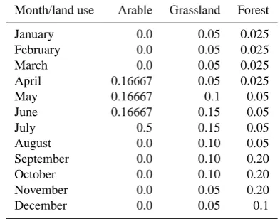
decom-position is sensitive to temperature and soil moisture. Hence, soil texture, monthly climate, land use and cultivation data are the inputs to the model (Coleman and Jenkinson, 1996; Smith et al., 1997). Three land use types are parameterized in RothC by default: arable, grassland and forest. They dif-fer in terms of plant input quality and the time distribution of plant inputs over the year. Plant quality determines the pro-portions of plant input that enter the DPM and RPM pool. The specific ratios of DPM/RPM are 1.44 for arable, 0.67 for grassland and 0.25 for forest. A lower ratio signifies greater decomposability with more plant material entering the DPM

Month/land use Arable Grassland Forest

January 0.0 0.05 0.025

February 0.0 0.05 0.025

March 0.0 0.05 0.025

April 0.16667 0.05 0.025

May 0.16667 0.1 0.05

June 0.16667 0.15 0.05

July 0.5 0.15 0.05

August 0.0 0.10 0.05

September 0.0 0.10 0.20

October 0.0 0.10 0.20

November 0.0 0.05 0.20

December 0.0 0.05 0.1

pool (fast turnover) and less entering the RPM pool (slow turnover). A higher ratio signifies the opposite. The distri-bution of plant inputs throughout the year for the three land use types mimics the dynamics of typical crop rotations and of permanent grassland or forest in Europe (Table 1). Over long time periods, the model is insensitive to the distribution of plant inputs throughout the year (Smith et al., 2005), so the distribution of inputs used for Europe was applied glob-ally. The total yearly input of C from plants, however, is an essential driver of SOC dynamics.

2.2 Climate data and scenarios (1901–2100)

Observed and predicted climate data are given on a monthly temporal, and 0.5 degree spatial resolution. From 1901 to 2005, observed climate data from CRU TS 3.0 were used. Scenario data spanned 2006 to 2100. The climate data were provided within the QUEST-GSI project and are avail-able online (http://www.cru.uea.ac.uk/∼_{timo/climgen/data/} questgsi/).

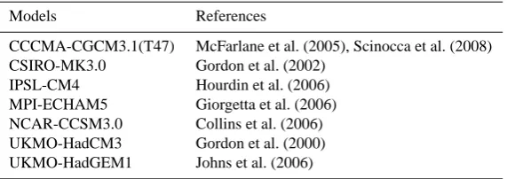
Table 2. Overview of GCMs used in this study.

Models References

CCCMA-CGCM3.1(T47) McFarlane et al. (2005), Scinocca et al. (2008) CSIRO-MK3.0 Gordon et al. (2002)

IPSL-CM4 Hourdin et al. (2006) MPI-ECHAM5 Giorgetta et al. (2006) NCAR-CCSM3.0 Collins et al. (2006) UKMO-HadCM3 Gordon et al. (2000) UKMO-HadGEM1 Johns et al. (2006)

2.3 Soil data

Mean SOC stocks in 0 cm to 30 cm depth and the percentage of clay are derived from the ISRIC-WISE global data set of derived soil properties (Version 3.0) on a 0.5 by 0.5 degree grid (Batjes, 2005). This data set interpolates soil characteris-tics of individual soil profile measurements from around the globe. These profile measurements were mainly taken in the decades of 1970 to 1990. Therefore, the SOC values used in this study represent the soil state roughly at the end of the last century. In this data set, each grid cell is covered by up to ten dominant soil types and gives their respective coverage in %. Each of these soil types was simulated consecutively in conjunction with the same input data within one scenario simulation. Results were aggregated over the different soil types per grid cell on an area-weighted basis. Since RothC is neither parameterised, nor recommended for use on organic soils, soils with SOC content higher than 200 cm (Smith et al., 2005) were omitted from the simulations.

2.4 Land use & land use change data

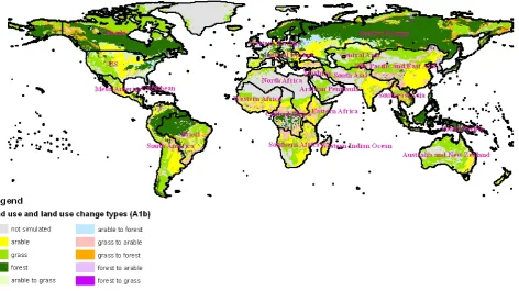
Gridded land use data as simulated by the Integrated Model to Assess the Environment (IMAGE) version 2.4 (MNP, 2006) were used in the RothC simulations. LUC in IMAGE is driven by (agro-)economic and climatic factors, such as changes in the demand for feed and food and the potential vegetation (MNP, 2006). IMAGE-data were available from 1970 onwards and we therefore also use 1970 as the start date for our simulations. Figure 1 shows the regional distri-bution of LUC between 1970 and 2100 exemplarily for the A1b scenario as deviations of LUC patterns among emission scenarios are small.

IMAGE simulates 20 land cover classes. These classes were classified into the three land use types which are imple-mented in RothC: arable, grassland and forestry. The classi-fication is shown in Table 3.

IMAGE simulations have the same spatial resolution of 0.5 degree as the climate data used in this study and each grid cell is considered to be homogeneous in terms of land

Table 3. Classification of IMAGE land use types into RothC land

cover classes. “−9999” denotes areas which were not simulated.

Land use (IMAGE 2.4) New Corresponding RothC land use code

Agricultural land 1 – arable Extensive grassland 2 – grassland C plantations (not used) No cells Regrowth forest (Abandoning) 3 – forest Regrowth forest (Timber) 3 – forest

Biofuel 1 – arable

Ice −9999

Tundra 2 – grassland

Wooded tundra 2 – grassland Boreal forest 3 – forest

Cool conifer 3 – forest

Temperate mixed forest 3 – forest Temperate deciduous forest 3 – forest Warm mixed forest 3 – forest Grassland/steppe 2 – grassland

Hot desert −9999

Scrubland 2 – grassland

Savannah 2 – grassland

Tropical woodland 3 – forest Tropical forest 3 – forest

use, LUC and NPP. Land use change patterns are given in 5-year time intervals.

2.5 Changes in soil carbon inputs according to changes in NPP

Fig. 1. Areas under the A1b scenario that are continuously covered by arable, grassland and forest from 1971 to 2100. Land use type changes

from 1971 to 2100 are depicted, neglecting intermediate changes. Note that the distributions of land use and land use change under SRES B1, A2, and B2 are very similar and are not plotted separately. Relevant differences are noted in the text.

the given environmental conditions. Once the plant inputs have been established in this way, the year-to-year changes are adjusted according to the year-to-year changes in NPP, because changes in C inputs to the soil can be associated with changes in NPP (Smith et al., 2005). Using the same approach as in Smith et al. (2005), we calculated changes in soil carbon inputs based on the changes in NPP data simu-lated by the IMAGE model version 2.4 (MNP, 2006). This scaling is appropriate as IMAGE-NPP also reflects changes in land cover change (see Sect. 2.4). Since land use change (amongst other factors) influences NPP changes in IMAGE, RothC uses these two drivers in a consistent way. The details of the simulation setup of this approach are described in the section “Simulation procedure”.

IMAGE NPP is a function of air temperature, soil mois-ture status, CO2-fertilisation, land cover and land cover

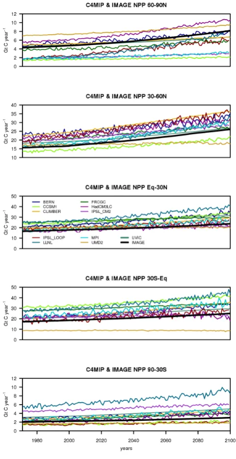
his-tory, nutrient availability, species characteristics and altitude (MNP, 2006). The carbon cycle model implemented in IM-AGE is thoroughly described in Klein Goldewijk et al. (1994) and has been successfully evaluated (Alcamo et al., 1994) and applied (Van Minnen et al., 2000, 2009) globally. Fur-ther, IMAGE NPP compares well with NPP results of the C4MIP study (Friedlingstein et al., 2006) in which dynamic global vegetation models coupled with AOGCMs were used to calculate (among others) NPP for the SRES A2 scenario. IMAGE NPP values of the SRES A2 scenario represent a medium scenario among the C4MIP scenarios for all global

zones (Fig. 2). IMAGE NPP data are again given in 5-year time intervals and are subsequently linearly interpolated for our study to yearly values between 1971–2100.

NPP surfaces to scale plant input values were only avail-able for the four SRES scenarios A1b, A2, B1 and B2, simulated by the IMAGE 2.4 model. To scale NPP values for the different temperature and precipitation trends of the seven AOGCM realisations of A1b, we associated the IM-AGE A1b NPP surface with the temperature and precipita-tion predicprecipita-tions of HadCM3, and scaled this baseline NPP surface according to the difference between the temperature and precipitation predictions from the other six AOGCMs and HadCM3, using the MIAMI-NPP model (Lieth, 1972). The MIAMI model links long-term average temperature and precipitation data with NPP via two simple regression func-tions (Lieth, 1972, 1975) derived from global NPP data sets, and has been applied globally to simulate NPP (e.g. Zheng et al., 2003).

The equations of the MIAMI-model are given by

NPP=min(NPPT,NPPP) (1)

with

Fig. 2. Comparison of zonal NPP of IMAGE and C4

MIP-simulations (Friedlingstein et al., 2006) for the SRES A2 emission scenario. Please refer to respective study for details on model ab-breviations.

term of NPP withT¯being annual mean temperature (◦_{C) and} NPPP is the moisture dependency term of NPP withP¯being the mean annual sum of precipitation (mm). NPP is either limited by temperature or precipitation, but this model does not account for the limiting effects when temperature or pre-cipitation is too high. The maximum NPP that can be reached is limited to 3000 g DM m−2yr−1. Absolute NPP values de-rived from MIAMI were not used directly, but were only used to scale IMAGE baseline NPP estimates.

IMAGE baseline NPP values were adjusted by the per-centage change, calculated by the MIAMI-NPP model, be-tween the baseline temperature/precipitation of HadCM3 and temperature/precipitation simulated by the other AOGCMs – within each 0.5 degree global grid cell and each year.

The following equation was used to scale NPP from the baseline IMAGE associated with HadCM3, to the NPP of the other six AOGCMs:

NPPAOGCMx=NPPIMAGE A1b (4)

+

NPPIMAGE A1b·

NPPMIAMI AOGCMx−NPPMIAMI HadCM3

NPPMIAMI HadCM3

where NPPAOGCMxis the AOGCM-specific NPP value with

x=1. . . 6, NPPIMAGE A1b is the NPP value of the IMAGE

baseline (here A1b) scenario, NPPMIAMI HadCM3is the NPP

value calculated by the MIAMI model with the tempera-ture of the AOGCM reference scenario (here HadCM3) and NPPMIAMI AOGCMx is the NPP value calculated by the

MI-AMI model with the temperature of the particular AOGCM scenario. A graphic example of the scaling approach for an arbitrary grid cell is given in Fig. 3.

2.6 Simulation procedure

The RothC model has previously been adapted to run with large spatial data sets and to use potential evapotranspiration (PET) in place of open pan evaporation (Smith et al., 2005). Since the modelling procedure is similar to that of Smith et al. (2005, 2006), only a brief description is given here. In the first initialisation step, RothC is run iteratively to equi-librium to calculate the sizes of the SOC pools and annual plant inputs using long-term average climate data (Coleman and Jenkinson, 1996) from 1901 to 1970. The model calcu-lates the soil pools and required C inputs according to the climate, land use, clay and SOC for 1970. In the forward run, from 1971 to 2100, climate, land use and C input changes determine SOC changes. C inputs are adjusted following the approach described in Smith et al. (2005):

PIt=PIt−1·

NPPt NPPt−1

(5)

where PIt is the plant C input in the given year (t C ha−1 yr−1), PIt−1is the plant C input in the previous year (t C ha−1

yr−1), NPPt is the NPP value for the given year (t C ha−1 yr−1_{) and NPP}

t−1 is the NPP value of the previous year

(t C ha−1_yr−1_{). Smith et al. (2005) note that it is}

uncer-tain whether C input to the soil changes proportionally with changes in NPP, and that the influence of NPP established here should be regarded as the maximum possible.

Fig. 3. Example of the NPP-scaling approach for an arbitrary grid cell. The panel on the left depicts NPP values calculated based on mean

yearly temperature and precipitation for the seven AOGCMs. The panel on the right shows the correspondingly scaled IMAGE-NPP values with HadCM3 being associated with the IMAGE-A1b-NPP surface.

(a) (b)

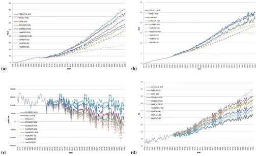
(c) (d)

Fig. 4. (a) Total global changes in mineral SOC for ten climate scenarios, (b) changes in global plant inputs for ten climate scenarios, (c)

were carried out including the effect of climate, land use and NPP change (default simulations).

2.7 Contribution of land use change to SOC stock changes

To examine the different influence of land use and NPP change on SOC, the HadCM3 model, in conjunction with SRES A1b, was run under three additional different set-ups: (a) simulation including the effect of LUC but keeping NPP constant over time, (b) simulation including the effect of NPP change but keeping the land use constant over time, and (c) simulation including neither change in NPP nor land use. The results of these additional simulations were then com-pared to the HadCM3 + SRES A1b simulation including both LUC and NPP change, which is the default set-up for all the other simulations (Sect. 2.6).

As previously stated, NPP and LUC are interlinked. NPP simulated by IMAGE differs not only according to temper-ature and precipitation change, but also according to LUC. Therefore, to simulate the effect of NPP alone without LUC, the NPP scaling based on IMAGE NPP cannot be used. In-stead, plant inputs were scaled according to the NPP change based on the calculation of MIAMI-NPP change. Simulation b follows this protocol. CO2-fertilisation is accounted for, as

although MIAMI-NPP changes do not account for the CO2

-fertilisation effect, MIAMI-NPP values are only used to scale IMAGE-NPP outputs, which do include CO2-fertilisation.

3 Results and discussion

3.1 Global mineral soil organic carbon dynamics

The initial sum of mineral SOC simulated in the first 30 cm of the soil amounts to ca. 502 Pg C in 1971. Global soils store

∼1550 Pg C (Lal, 2004) of which ca. 53 % (global average) is distributed in the first 30 cm of the soil profile (Jobbagy and Jackson, 2000), which is 821.5 Pg C. The simulated value ex-cludes all soils with a SOC density higher than 200 t ha−1at the start and end of the simulation, i.e. all organic soils that contain 412 Pg to 1 m (Joosten, 2009), so the difference be-tween the soil C accounted for is due to the exclusion of these soils.

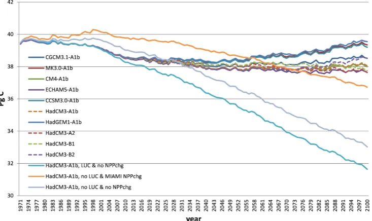
Our simulations, including changes in climate, land use and NPP, suggest that aggregate global mineral SOC stocks continuously increase from 1971 up to 2100 with varying in-tensity in all scenarios except one, i.e. HadCM3-B1 (Fig. 4a). In the latter, SOC begins to level-out towards the end of this century. This steady increase over time is driven by increas-ing plant inputs projected by the IMAGE model (Fig. 4b) and a negative trend in the global climatic water balance (Fig. 4c), which reduces soil moisture, and will tend to slow organic matter decomposition. These two effects override the increase in decomposition rate arising from increased tem-perature (Fig. 4d).

Although SOC trends are consistently positive using the different AOGCMs and SRES scenarios, there is a consider-able spread between the scenarios. Across all simulations, SOC increases between 26.4 and 81.2 Pg SOC-C with a corresponding spread of 54.8 Pg C. While SOC stocks in-crease between 46.8 to 81.2 Pg C within the seven AOGCMs (spread = 34.5 Pg C), the HadCM3 simulations driven by four SRES scenarios show a lower SOC stock gain from 26.4 to 48.6 Pg C (spread = 22.2 Pg C). Figure 4a also shows that the SOC response to the HadCM3 climate scenario ranges at the lower end of all other AOGCMs responses, and therefore also the SRES realisations A2, B1 and B2 with HadCM3.

With a simulated consistent increase of global mineral SOC during the 21st century, our results are generally in agreement with the works of Cramer et al. (2001), Friedling-stein et al. (2006), Ito (2005), Lucht et al. (2006), M¨uller et al. (2007) and Sitch et al. (2008), of which Friedlingstein et al. (2006) and Sitch et al. (2008) are coupled simulation stud-ies. Our results are, however, in disagreement with Jones et al. (2005) and Schaphoff et al. (2006) (Table 4).

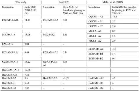
Absolute SOC stock changes cannot be directly compared as we are only considering the first 30 cm of the soil profile and the other studies consider total soil profiles (or to 1m depth), and include areas covered by organic soils (although none treated organic soils differently to mineral soils), but percentage change can be compared. Cramer et al. (2001) use the IS92a anthropogenic emission scenario, which is com-parable to the later IPCC A1b scenario in conjunction with the HadCM2-SUL version of the Hadley Centre AOGCM. Their simulations show a ca. 10% increase (mean of six DGVM) between 2000 and 2100, while our simulation of the A1b simulation driving the HadCM3 AOGCM results in a mean increase of ca. 8% of SOC stocks. Ito (2005) simulates, amongst others, SOC stock changes for the 21st century us-ing seven AOGCMs driven by the IPCC A2 scenario. Most AOGCMs are the same as those used in this study, but are earlier versions, and Ito (2005) simulated the A2 emissions scenario (lower climate forcing), whereas we largely used the A1b scenario (higher climate forcing). As expected, the percentage changes from Ito, 2005, are considerably smaller than the changes suggested in this study (Table 5).

However, in both studies, the AOGCMs rank similarly, with the climate from the NCAR model giving greatest SOC increase, and the climate as simulated by the Australian MK model giving the second highest increase. The simulation re-sults using the Hadley Centre model climate forcing, both driven by the IPCC A2 emission scenario, give contradictory results; our results show a slight increase in SOC, whereas the study of Ito (2005) shows a decrease.

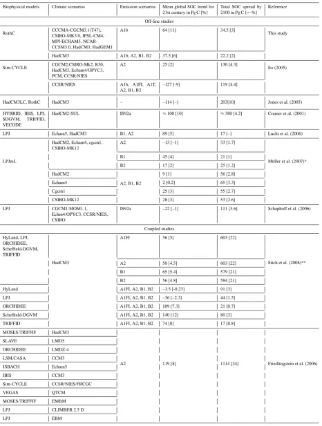
Off-line studies RothC CCCMA-CGCM3.1(T47),

CSIRO-MK3.0, IPSL-CM4, MPI-ECHAM5, NCAR-CCSM3.0, HadCM3, HadGEM1

A1b 64 [11] 34.5 [3]

This study

HadCM3 A1b, A2, B1, B2 37.5 [6] 22.2 [2] Sim-CYCLE CGCM2,CSIRO-Mk2, R30,

HadCM3, Echam4/OPYC3, PCM, CCSR/NIES

A2 25 [2] 130 [4.3]

Ito (2005)

CCSR/NIES A1b, A1FI, A1T, A2, B1, B2

–127 [-9] 119 [4.4]

HadCM3LC, RothC HadCM3 – –114 [–] 203[10] Jones et al. (2005) HYBRID, IBIS, LPJ,

SDGVM, TRIFFID, VECODE

HadCM2-SUL IS92a ≈100 [10] ≈380 [4.2] Cramer et al. (2001)

LPJ Echam5, HadCM3 B1, A2 89 [5] 17 [–] Lucht et al. (2006)

LPJmL

HadCM2, Echam4, cgcm1, CSIRO-MK12

A2 –13 [–1] 33 [1.7]

M¨uller et al. (2007)* B1 45 [4] 21 [1]

B2 17 [2] 25 [1.2] HadCM2

A2, B1, B2

9 [1] 56 [2.8] Echam4 2 [0.2] 65 [3.3] Cgcm1 25 [3] 55 [2.7] CSIRO-MK12 28 [3] 53 [2.6] LPJ CGCM1/MOM1.1,

Echm4/OPYC3, CCSR/NIES, CSIRO

IS92a –22 [–1] 111 [3.6] Schaphoff et al. (2006)

Coupled studies HyLand, LPJ,

ORCHIDEE, Scheffield-DGVM, TRIFFID

HadCM3

A1FI 56 [5] 603 [22]

Sitch et al. (2008)** A2 50 [4.5] 603 [22]

B1 65 [5.4] 579 [21] B2 56 [4.8] 584 [21] HyLand A1FI, A2, B1, B2 –3.5 [-0.23] 91 [3] LPJ A1FI, A2, B1, B2 –36 [–2.3] 44 [1.5] ORCHIDEE A1FI, A2, B1, B2 109 [7.3] 21 [0.7] Scheffield-DGVM A1FI, A2, B1, B2 140 [12] 80 [3] TRIFFID A1FI, A2, B1, B2 74 [8] 17 [0.8] MOSES/TRIFFIF HadCM3

A2 119 [8] 1114 [34] Friedlingstein et al. (2006) SLAVE LMD5

ORCHIDEE LMDZ-4 LSM,CASA CCM3 JSBACH Echam5 IBIS CCM3

Sim-CYCLE CCSR/NIES/FRCGC VEGAS QTCM

MOSES/TRIFFIF EMBM LPJ CLIMBER 2.5 D LPJ EBM

* Results from simulations which include changes in land use, atmospheric CO2and climate.

Table 5. Simulated changes of global SOC stocks in the 21st century in % for the ten simulations of our study and the comparable studies

of Ito (2005) and M¨uller et al. (2007). Please note that, except the simulations with the Hadley Centre AOGCM, the simulations differ in the driving anthropogenic emission scenario: A1b for our study and A2 for the study of Ito (2005) and A2, B1 and B2 for the study of M¨uller et al. (2007).

This study Ito (2005) M¨uller et al. (2007)

Simulation Delta SOC 2000–2100 (%)

Simulation Delta SOC for decades beginning in 2000 and 2090 (%)

Simulation Delta SOC for decades beginning in 1970 and 2091(%)

CGCM3.1-A1b 11.11 CGCM2.0-A2 0.81

CGCM1 - A2 –0.3

CGCM1 - B1 5.2

CGCM1 - B2 2.6

MK3.0-A1b 13.06 MK2.0-A2 1.69

MK1.2 - A2 0.2

MK1.2 - A2 5.5

MK1.2 - A2 2.9

CM4-A1b 9.04 – –

ECHAM5-A1b 9.64 ECHAM4-A2 0.34

ECHAM4-A2 -3.1

ECHAM4-B1 3.4

ECHAM4-B2 0.4

CCSM3.0-A1b 14.22

NCAR-PCM-A2

6.96 – –

HadGEM1-A1b 12.66 – – – –

HadCM3-A1b 7.51 – – – –

HadCM3-A2 3.5 HadCM2-A2 –1.89 HadCM2 - A2 –2

HadCM3-B1 6.51 - - HadCM2 - B1 4

HadCM3-B2 7.86 – – HadCM2 - B2 1

2011), respectively, while our A2 simulations show a 3.5 % increase. Results of the C4MIP study, in which 11 coupled climate-carbon-cycle models were forced by the A2 emission scenario (Friedlingstein et al., 2006), show a mean increase of global SOC of 8 % compared to 3.5 % in our HadCM3-A2 simulation.

Mean SOC stock trends predicted by six DGVMs driven by HadCM3 climate and four SRES scenarios – namely A1FI, A2, B1 and B2 – are +5, 4.5, 5.4 and 4.8 %, respec-tively (Sitch et al., 2008) (Table 4), while our simulated SOC increases using HadCM3 are +7.5, 3.5, 6.5 and 7.9 % (Table 5).

M¨uller et al. (2007) use the LPJmL model, driven by SRES scenarios A2, B1 and B2 and realisations of the AOGCMs HadCM2, ECHAM4, CGCM1 and CSIRO-MK1.2, to simu-late changes of the land carbon balance during the 21st cen-tury, while also considering land use change patterns derived from the IMAGE model. Simulations with the HadCM2 model and emission scenarios A2, B1 and B2 show an overall smaller increase of global SOC and even a decrease under A2 compared to our results (Table 5). This could be explained by the fact that the impact of land use change on SOC in their

driven by the same climate and emission scenario. The study of Sitch et al. (2008) predicts a spread in SOC values by 2099 of 21 and 22%. Variability of simulated SOC stocks by 2100 by Friedlingstein et al. (2006) with 11 AOGCMs and each coupled with a different biophysical carbon-cycle model is even higher with 34 %. With the exception of the results by Cramer et al. (2001), this suggests that the variability in pre-dictions of global SOC is higher due to the difference among the implementations of carbon-cycle dynamics than due to uncertainties in climate forcings and emission scenarios. 3.2 Contribution of land use change to SOC stock

changes

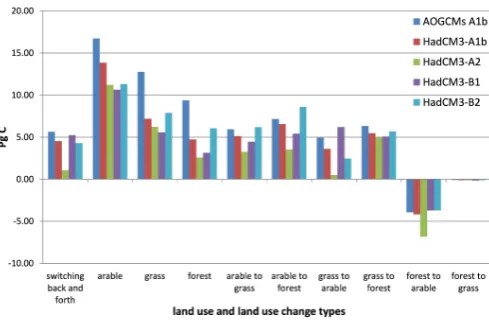
Land use change occurs on 19 % of the land area under the A1b scenario, and on 17 %, 19% and 17 % of the land under the B1, A2 and B2 scenarios, respectively. Simulations in-cluding the effects of climate, LUC and NPP together suggest LUCs from forest to arable constitute the largest SOC losses, while forest to grassland losses are negligible, in keeping with previous meta-analyses of LUC impacts on SOC (Guo and Gifford, 2002). All other types of LUC gain C, even grass to arable. This might constitute an artefact since our simula-tions do not include the negative impact of the removal of harvested biomass and residue. However, continuous arable soils seem to have the highest gain in organic C compared to grass and forest soils (Fig. 5), which might override losses due to biomass removal after land use change from grass to arable in the long term. Grassland to arable conversion is known to decrease SOC stocks (Guo and Gifford, 2002), but over the course of the simulations (130 years), increased NPP and/or decreased decomposition due to limiting soil mois-ture counteract these losses in some locations (Table 6), re-sulting in an overall global increase in mineral SOC despite the LUC-driven losses. Some grassland to arable conversions lose SOC and others gain, but due to NPP increases in some regions, the aggregate global change is a net increase in SOC. This net result would hold even if SOC losses due to the con-version of grass to arable were negative to the same extent as the SOC losses due to the conversion of forest to arable.

Figure 6 shows an assessment of the contribution of land use and NPP change to the projected SOC stock changes us-ing HadCM3 with emission scenario A1b. Comparison of the simulation using fixed NPP in conjunction with changing land use, and the simulation that includes neither land use nor NPP change, shows that the impact of LUC on global SOC stocks is negligible. Figure 1 shows the distribution of simulated LUCs occurring from 1971 to 2100. The simula-tion using fixed land use plus changing NPP shows that an NPP increase forced by climate change only would lead to a decrease in global SOC. The difference between the

sim-Fig. 5. Contribution of land use and land use change to global SOC

stock changes (from 1971 to 2100).

ulation using fixed land-use plus NPP change and the de-fault HadCM3 simulation approximately represents the ef-fect of CO2-fertilisation. The increase in NPP due to CO2

-fertilisation could therefore be a dominant factor in determin-ing whether SOC stocks continue to act as a sink of C in the future. This has also been shown for forest soils in Northeast China by Peng et al. (2009), who conducted a simulation with and without the CO2-fertilisation effect and showed a

contin-uous loss of SOC from 2000 to 2100 without CO2

fertilisa-tion, but an increase in forest SOC if CO2-fertilisation is

in-cluded. Carbon losses were reduced by the CO2-fertilisation

effect compared to the simulation without, in the study of Smith et al. (2009), for Canadian arable soils.

3.3 Regional trends in SOC dynamics

During the following discussion, environmental, SOC and plant input trends always refer to the average of all simula-tions, if not otherwise explicitly stated. Regions are as shown in Fig. 1.

Fig. 6. Simulated changes in SOC stocks for four experimental set-ups using the climate scenario data of the HadCM3 AOGCM in

con-junction with A1b. Blue line: simulation including land use and NPP change; the latter is based on IMAGE NPP which includes the CO2

-fertilisation effect. Green line: simulation including no land use change but NPP change; the latter is based on temperature and precipitation changes only. Purple line: simulation including neither land use nor NPP change. Red line: simulation including land use change but no NPP change.

on SOC stock for the NW Pacific and E Asia compared to the whole globe. About 25 % (20 %-B1, 20 %-B2, 21 %-A2) of the area undergoes LUC, of which about 15 % (15.5 %-B1, 9.7 %-B2, 10.5 %-A2) is the conversion from grass to arable and about 9 % (9 %-B1, 8.5 %-B2, 9 %-A2) is the conversion from forest to arable. The area as a whole shows the highest negative impact of LUC on SOC stocks compared to all other regions.

SOC losses in Northeast China and North and South Ko-rea can be mainly attributed to LUC from forest to arable, while the belt of losses of SOC is due to changes from mainly grassland to arable conversions. Both changes are driven by decreasing plant inputs (Fig. 9).

The region as a whole shows a distinct SOC dynamic com-pared to other regions and the rest of the globe. While SOC trends of most regions show a continuous increase from 1971 to 2100, NW Pacific and E Asia show first a drop of SOC until ca. 2060 and thereafter a slight increase (Fig. 8). This pattern is caused by the C losses due to conversion to arable in the first part of the 21st century, which stabilises there-after followed by a steady increase of arable SOC stocks during the 21st century (data not shown). A very similar pat-tern has also been simulated for forests soils in Northeast-ern China by Peng et al. (2009). Peng et al. (2009) used a dedicated forest model (TRIPLEX 1.0) including the CO2

-fertilisation effect on biomass production and climate sce-nario inputs from CGCM3.1 in conjunction with (among oth-ers) SRES A1. They also simulate a decrease in SOC levels from 2000 to ca. 2040 and thereafter a steady increase, but this is not due to LUC. No interpretation of these results is given. However, if we aggregate our results for continuous forest soils of the CGCM3.1 A1b simulation in NW Pacific and E Asia, we see a continuous loss of SOC. This difference to the study of Peng et al. (2009) is due to two factors (a) in the current study, plant inputs (i.e. NPP) remain fairly con-stant while Peng et al. (2009) simulate a continuous increase in biomass, and (b) in the current study, the temperature in-crease is stronger than in Peng et al. (2009) and hence plant inputs are driven by a lower temperature increase than in our CGCM3.1 A1b simulation (data not shown).

3.3.2 Northern high latitudes, boreal forests and grasslands

Under a warmer climate, soil organic matter decomposition increases if soil moisture is not limiting. These circumstances cause widespread SOC losses in Eurasia, Canada and Alaska as also shown by Schaphoff et al. (2006). These losses dom-inate the mean total mineral SOC response in the northern high latitudes (NHL), which is only slightly positive over the course of the simulation with an average increase over

10 %, whereas our HadCM3-A2 simulation predicts a total loss of mineral SOC of –3.1%. This is however in agreement with the simulations of Jones et al. (2005) with HadCM3 and RothC, which predict a total SOC loss for the NHL of –5 %. This suggests that mineral SOC dynamics as simulated with RothC is more sensitive to increasing temperatures in the northern latitudes than the SOC dynamic implementations of the C4MIP models. Furthermore, Qian et al. (2010)

explic-itly point out that the “apparent “suppression” of warming-induced increase in SOM decomposition in the C4MIP

mod-els still comes as somewhat of a surprise”. Carbon losses in the area of Sweden are amplified due to the almost zero increase in plant inputs. However, central Canada’s forests increase in SOC, because the temperature increase is more moderate and, although plant inputs are not higher than in the previously mentioned forest areas, they are large enough to counteract the SOC losses induced by higher temperature. The same applies to northern grasslands which generally gain SOC through temperature increases between 5 and 8◦C. Soil organic C also increases under the northward shift of forests into grasslands. This is in agreement with simulation results using LPJ by Schaphoff et al. (2006), which predict an in-crease of SOC in central and Northern Canada.

The expansion of forest in conjunction with increased plant inputs in the area around Moscow triggers substantial SOC gains.

3.3.3 Canada

Fig. 8. Dynamic of total SOC changes aggregated over the region of NW Pacific and E Asia of all simulations (see text for further details).

North Africa 23.50 513.07 422.28 – – – −25.81 98.08 −8.64 – Western Africa 117.15 710.27 826.22 53.88 4.81 – 37.79 235.76 −160.53 – Central Africa 506.54 548.26 288.74 1426.60 – – 860.04 748.90 −739.51 – Eastern Africa 43.15 1087.19 374.42 −4.24 – – 159.00 27.03 −45.95 – Western Indian Ocean 0.00 492.44 37.83 −7.03 – – 225.21 – −99.34 – Southern Africa 88.94 2189.28 1163.00 3.46 82.45 – 2835.80 43.11 73.32 – South Asia 75.45 32.90 179.55 −85.17 – – −214.92 −13.68 −164.97 −7.81 Southeast Asia 256.42 678.92 560.26 1806.26 – – 301.61 721.08 −141.06 0.52 NW Pacific and East Asia 33.76 1483.53 −46.25 −151.62 2.04 65.28 −423.58 3.32 −1708.21 −35.36 Central Asia 19.48 187.49 722.09 −3.50 1784.80 73.28 −6.71 21.07 – – Australia and New Zealand 551.04 344.17 681.08 −0.03 875.26 −11.53 34.30 −16.54 −14.38

South Pacific 0.00 4.00 – 126.71 – 0.67 – 2.70 −165.95

Western Europe 240.48 515.07 168.69 −963.97 201.28 1101.84 1.68 90.94 3.03 −14.67 Central Europe 90.99 533.36 53.78 31.09 38.74 678.64 −263.28 2.36 −6.86 −3.35 Eastern Europe 610.06 1368.61 251.14 −2326.09 833.17 3101.82 20.67 1071.02 −91.79 −18.70

Arabian Peninsula −2.69 – 770.69 – – – – – – –

Mashriq −1.70 40.08 70.52 – – – −24.14 – – –

Canada 62.15 134.56 545.65 −849.75 93.04 330.96 9.27 776.40 −171.71 −4.90 US 318.12 837.05 446.88 −546.72 1893.97 1573.90 44.46 310.14 −5.88 −14.99

Caribbean 0.02 169.33 0.01 35.44 – – 6.32 24.15 1.56

Mesoamerica 252.54 1203.11 171.27 501.10 – – 222.98 12.17 −6.68 12.13 Brazil 1867.38 1776.55 3998.25 7172.83 88.37 237.69 645.00 1569.18 −83.91 1.97 South America 482.96 1873.73 1075.89 3159.57 36.77 – 532.32 545.51 −386.58 15.59

Fig. 10. Regional trends of average (of all scenarios) total SOC stocks, SOC concentrations and % change and respective minimum and

maximum values of all scenarios.

3.3.4 USA

Arable areas in central US and grassland areas in Western US areas profit from climate change in conjunction with in-creased plant inputs. However, the large forest areas situated in wetter parts of the future US lose SOC, despite generally

Fig. 11. Spatial distribution of the difference between the uncertainty in SOC stocks of AOGCM and SRES simulations. Uncertainty is

calculated as the maximum spread between SOC results in 2100 among the AOGCM simulations and the SRES simulations respectively.

3.3.5 South America and Brazil

SOC stocks increase in most of South America and Brazil in the future, despite higher temperature of up to +7–8◦_{C in the} centre of the continent. The water balance decreases in the north substantially, while some areas in middle and southern South America become much wetter than in 1971. Plant in-puts increase on the whole continent and most prominently in eastern Brazil, where the highest SOC stock increases glob-ally are found (Fig. 10). Only the lee side of the southern Andes shows a moderate decline in SOC, which correlates with increased plant inputs close to zero.

3.3.6 Europe

The whole of Europe shows moderate SOC gains. Moder-ately to highly increased plant inputs counteract enhanced SOM turnover under a warmer climate, where soil moisture is not a limiting factor. Hence, here these two processes tend to cancel each other out, as suggested by other studies for Western Europe (Smith et al., 2005, 2006).

3.3.7 Africa

Africa shows only two distinct areas of SOC losses. In central Africa, they are due to deforestation and conversion to arable in conjunction with hence lower plant inputs. In the south, SOC is lost due to increased soil organic matter decomposi-tion under grassland, where the slightly increased plant in-puts cannot counteract the losses. Arable soils and soils un-der grass to arable conversion profit from the overriding ef-fect of increasing plant inputs over increased decomposition in the future. Also the simulations by Schaphoff et al. (2006) predict slight SOC gains in the Sahel zone due to a shift to C4 grasses support increasing NPP and dry conditions, and therefore limiting SOC turnover.

3.3.8 India

Fig. 12. Spatial distribution of areas where (a) the GCM simulation produces agreement on SOC becoming a source or a sink in 2100 when

soils, because the local high increases in SOC are not out-weighed by the widespread small losses.

3.3.9 Australia

Australia tends to lose SOC around its central desert area where grasslands are predicted to become drier and warmer in the future. The rate of SOC decomposition is slowed down under the drier conditions, and SOC stocks could increase here with a small increase in plant inputs. However, the tem-perature effect seems to outweigh the potential SOC gains. By contrast, the arable soils tend to increase in SOC due to the predicted increases in plant inputs. This is consistent with most other arable regions in our simulations.

3.4 Consistency among simulations in predicting future SOC stocks

The consistency among simulations shows considerable re-gional variation (Fig. 10). Regions such as the Arabian Peninsula, the Caribbean, central Africa and Mesoamerica have the highest local uncertainty in terms of how SOC con-centrations develop in the future, but this uncertainty is not reflected in a global uncertainty, because these regions have a relatively small contribution to the total SOC stocks. By contrast, Brazil shows the third highest uncertainty in fu-ture changes in SOC concentration, but also the highest to-tal SOC stock uncertainty, due to very high SOC gains. We can therefore distinguish between locally important uncer-tainties in the prediction of SOC stocks, which could impact people’s livelihoods, and uncertainties which impact more on the global climate development. SOC predictions where soils become a source or sink in the future are highly uncertain in regions where some scenarios predict SOC losses and some scenarios predict SOC gains, such as in Canada, Eastern Eu-rope, NW Pacific and E Asia, South Asia, South Pacific and Western Africa (Fig. 10).

Figure 11 shows the spatial distribution of the difference between the uncertainty of the AOGCM A1b simulations,and the HadCM3 SRES scenario simulations. The uncertainty is defined as the spread of SOC stock values of one set of simulations in 2100. A greater uncertainty in SOC between AOGCM runs than for the SRES predictions, for example in the Amazon region, reflects an inconsistency between the AOGCM climate projections. In these cases, the uncertainty in SOC introduced by different climate models is greater than the uncertainty introduced by GHG emission pathway sce-narios.

Many of the simulations show agreement (Fig. 12) as to whether soils are predicted to act as a source or sink across climate models (a) and across SRES scenarios (b). The stronger the agreement between simulations, the higher is the probability that these results are robust with respect to the climate variable used to drive RothC. The maps do not, however, show the magnitude of SOC changes.

4 Conclusions

Globally, under a warming climate, increases are seen both in C inputs to the soil due to higher NPP, and in SOC losses due to increased decomposition (where soil moisture is not limiting). The balance between these processes defines the change in SOC stock. In some regions the processes balance, but in others, one process is affected by climate more than the other. This study suggests, with high probability, that in most parts of the world SOC stocks will change, with SOC losses projected to occur in northern latitudes where a higher SOC decomposition due to higher temperatures is not bal-anced by increased NPP, whereas in tropical regions, NPP increases override losses due to higher SOC decomposition. Pronounced regional trends are visible within this global pic-ture. The spatial heterogeneity in the response of SOC to changing climate shows how delicately balanced the com-peting gain and loss processes are, with subtle changes in temperature, moisture, soil type and land use interacting to determine whether SOC increases or decreases in the future. Given this delicate balance, we should stop asking the gen-eral question of whether soils will increase or decrease in SOC under future climate, as there appears to be no single answer. Instead, we should focus our efforts on improving our prediction of factors that determine the size and direc-tion of change, and the land management practices that can be implemented to protect and enhance SOC stocks as dis-cussed in Smith (2008).

Acknowledgements. We thank the National Environment Research Council UK for funding this research through the QUEST-GSI Project. Pete Smith is a Royal Society-Wolfson Research Merit Award holder. This paper also contributes to the EU FP7-funded CCTAME, CarboExtreme and GHG-Europe projects, and to Scotland’s ClimateXChange.

Edited by: J. Leifeld

References

Alcamo, J., Kreileman, G. J. J., Krol, M. S., and Zuidema, G.: Mod-eling the global society-biosphere-climate system: Part 1: Model description and testing, Water, Air, Soil Pollut., 76, 1–35, 1994. Batjes, N. H.: ISRIC-WISE global data set of derived soil properties

an a 0.5 by 0.5 degree grid (Version 3.0). Report 2005/08, ISRIC – World Soil Information, Wageningen (with data set), 2005. Berthelot, M., Friedlingstein, P., Ciais, P., Dufresne, J.-L., and

Mon-fray, P.: How uncertainties in future climate change predictions translate into future terrestrial carbon fluxes, Glob. Change Biol., 11, 959–970, 2005.

Coleman, K. W., and Jenkinson, D. S.: RothC-26.3 - A model for the turnover of carbon in soil., in: Evaluation of soil organic matter models using existing long-term datasets, edited by: Powlson, D. S., Smith, P., and Smith, J., NATO ASI Series I, Springer-Verlag, Heidelberg, 237–246, 1996.

Collins, W. D., Bitz, C. M., Blackmon, M. L., Bonan, G. B., Bretherton, C. S., Carton, J. A., Chang, P., Doney, S. C., Hack, J. J., Henderson, T. B., Kiehl, J. T., Large, W. G., McKenna, D. S., Santer, B. D., Smith, R. D.: The Community Climate System Model Version 3 (CCSM3), J. Clim., 19, 2122–2143, 2006. Cox, P. M., Betts, R. A., Jones, C. D., Spall, S. A., and Totterdell,

I. J.: Acceleration of global warming due to carbon-cycle feed-backs in a coupled climate model, Nature, 408, 184–187, 2000. Cramer, W., Bondeau, A., Woodward, F. I., Prentice, I. C., Betts,

R. A., Brovkin, V., Cox, P. M., Fisher, V., Foley, J. A., Friend, A. D., Kucharik, C., Lomas, M. R., Ramankutty, N., Sitch, S., Smith, B., White, A., and Young-Molling, C.: Global response of terrestrial ecosystem structure and function to CO2and

cli-mate change: results from six dynamic global vegetation models, Glob. Change Biol., 7, 357–373, 2001.

Davidson, E. A. and Janssens, I. A.: Temperature sensitivity of soil carbon decomposition and feedbacks to climate change, Nature, 440, 165–173, 2006.

Diels, J., Vanlauwe, B., Van der Meersch, M. K., Sanginga, N., and Merckx, R.: Long-term soil organic carbon dynamics in a sub-humid tropical climate: 13C data in mixed C3/C4 cropping and modeling with ROTHC, Soil Biol. Biochem., 36, 1739–1750, 2004.

Dufresne, J. L., Fairhead, L., Le Treut, H., Berthelot, M., Bopp, L., Ciais, P., Friedlingstein, P., and Monfray, P.: On the magnitude of positive feedback between future climate change and the carbon cycle, Geophys. Res. Lett., 29, 1405, 2002.

Eglin, T., Ciais, P., Piao, S. L., Barre, P., Bellassen, V., Cadule, P., Chenu, C., Gasser, T., Koven, C., Reichstein, M., and Smith, P.: Historical and future perspectives of global soil carbon response to climate and land-use changes, Tellus B, 62, 700–718, 2010. Falloon, P., and Smith, P.: Simulating SOC changes in long-term

experiments with RothC and CENTURY: model evaluation for a regional scale application, Soil Use Manage., 18, 101–111, doi:10.1111/j.1475-2743.2002.tb00227.x, 2002.

Falloon, P. D., Smith, P., Smith, J. U., Szab´o, J., Coleman, K., and Marshall, S.: Regional estimates of carbon sequestration poten-tial: linking the Rothamsted Carbon Model to GIS databases, Biol. Fertil. Soils, 27, 236–241, 1998.

Fang, C., Smith, P., Moncrieff, J. B., and Smith, J. U.: Similar re-sponse of labile and resistant soil organic matter pools to changes in temperature, Nature, 433, 57–59, 2005.

Friedlingstein, P., Dufresne, J. L., Cox, P. M., and Rayner, P.: How positive is the feedback between climate change and the carbon cycle?, Tellus B, 55, 692–700, 2003.

Friedlingstein, P., Cox, P., Betts, R., Bopp, L., von Bloh, W., Brovkin, V., Cadule, P., Doney, S., Eby, M., Fung, I., Bala, G., John, J., Jones, C., Joos, F., Kato, T., Kawamiya, M., Knorr, W., Lindsay, K., Matthews, H. D., Raddatz, T., Rayner, P., Re-ick, C., Roeckner, E., Schnitzler, K. G., Schnur, R., Strassmann,

Giorgetta, M.A., Brasseur, G.P., Roeckner, E., Marotzke, J.: Preface to Special Section on Climate Models at the Max Planck Institute for Meteorology, J. Clim. 19, 3769–3770, 2006.

Gordon, C., Cooper, C., Senior, C. A., Banks, H., Gregory, J. M., Johns, T. C., Mitchell, J. F. B., and Wood, R. A.: The simulation of SST, sea ice extents and ocean heat transports in a version of the Hadley Centre coupled model without flux adjustments, Clim. Dynam., 16, 147–168, 2000.

Gordon, H. B., Rotstayn, L. D., McGregor, J. L., Dix, M. R., Koal-czyk, E. A., O’Farrell, S. P., Waterman, L. J., Hirst, A. C., Wil-son, S. G., Collier, M. A., WatterWil-son, I. G., and Elliott, T. I.: The CSIRO Mk3 Climate System Model [Electronic publica-tion]. Aspendale: CSIRO Atmospheric Research, Technical pa-per no. 60, 130 pp., 2002.

Guo, L. B. and Gifford, R. M.: Soil carbon stocks and land use change: a meta analysis, Glob. Change Biol., 8, 345–360, doi:10.1046/j.1354-1013.2002.00486.x, 2002.

Hourdin, F., Musat, I., Bony, S., Braconnot, P., Codron, F., Dufresne, J.-L., Fairhead, L., Filiberti, M.-A., Friedlingstein, P., Grandpeix, J.-Y., Krinner, G., LeVan, P., Li, Z.-X., Lott, F.: The LMDZ4 general circulation model: climate performance and sensitivity to parametrized physics with emphasis on tropical convection, Clim. Dynam., 27, 787–813, 2006.

Ito, A.: Climate-related uncertainties in projections of the twenty-first century terrestrial carbon budget: off-line model experi-ments using IPCC greenhouse-gas scenarios and AOGCM cli-mate projections, Clim. Dynam., 24, 435–448, 2005.

Jenkinson, D. S., Adams, D. E., and Wild, A.: Model estimates of CO2emissions from soil in response to global warming, Nature,

351, 304–306, 1991.

Jenkinson, D. S., Harris, H. C., Ryan, J., McNeill, A. M., Pilbeam, C. J., and Coleman, K.: Organic matter turnover in a calcareous clay soil from Syria under a two-course cereal rotation, Soil Biol. Biochem., 31, 687–693, 1999.

Jobbagy, E. G. and Jackson, R. B.: The Vertical Distribution of Soil Organic Carbon and Its Relation to Climate and Vegetation, Ecol. Appl., 10, 423–436, 2000.

Johns, T. C., Durman, C. F., Banks, H. T., Roberts, M. J., McLaren, A. J., Ridley, J. K., Senior, C. A., Williams, K. D., Jones, A., Rickard, G. J., Cusack, S., Ingram, W. J., Crucifix, M., Sexton, D. M. H., Joshi, M. M., Dong, B. W., Spencer, H., Hill, R. S. R., Gregory, J.M., Keen, A. B., Pardaens, A. K., Lowe, J.A., Bodas-Salcedo, A., Stark, S., Searl, Y.: The New Hadley Centre Cli-mate Model (HadGEM1): Evaluation of Coupled Simulations, J. Clim., 19, 1327–1353, 2006.

Jones, C., McConnell, C., Coleman, K., Cox, P., Falloon, P., Jenkin-son, D., and PowlJenkin-son, D.: Global climate change and soil carbon stocks; predictions from two contrasting models for the turnover of organic carbon in soil, Glob. Change Biol., 11, 154–166, doi:10.1111/j.1365-2486.2004.00885.x, 2005.

Kamoni, P. T., Gicheru, P. T., Wokabi, S. M., Easter, M., Milne, E., Coleman, K., Falloon, P., Paustian, K., Killian, K., and Ki-handa, F. M.: Evaluation of two soil carbon models using two Kenyan long term experimental datasets, Agr. Ecosyst. Environ., 122, 95–104, 2007.

Klein Goldewijk, K., Minnen, J. G., Kreileman, G. J. J., Vloedbeld, M., and Leemans, R.: Simulating the carbon flux between the ter-restrial environment and the atmosphere, Water, Air, Soil Pollut., 76, 199–230, 1994.

Knorr, W., Prentice, I. C., House, J. I., and Holland, E. A.: Long-term sensitivity of soil carbon turnover to warming, Nature, 433, 298–301, 2005.

Lal, R.: Soil erosion and the global carbon budget, Environ. Int., 29, 437–450, doi:10.1016/s0160-4120(02)00192-7, 2003.

Lal, R.: Soil carbon sequestration impacts on global climate change and food security, Science, 304, 1623–1627, 2004.

Lieth, H.: The primary productivity of the world, Nature and Re-sources UNESCO, VIII, 5–10, 1972.

Lieth, H.: Modelling the primary productivity of the world, in: Pri-mary productivity of the Biosphere, edited by: Lieth, H., and Whittaker, R. H., Springer-Verlag, New York, 237–263, 1975. Lucht, W., Schaphoff, S., Erbrecht, T., Heyder, U., Cramer, W.:

Ter-restrial vegetation redistribution and carbon balance under cli-mate change, Carbon Balance and Management, p. 7, 2006. McFarlane, N. A., Scinocca, J. F., Lazare, M., Harvey, R. Verseghy,

D., Li, J.: The CCCma third generation atmospheric general cir-culation model. CCCma Internal Report, 25 pp, 2005.

McGill, W. B.: Review and classification of 10 soil organic mat-ter (SOM) models, in: Evaluation of Soil Organic Matmat-ter models Using Long-Term Datasets, NATO ASI Series I, edited by: Powl-son, D. S., Smith, P., and Smith, J., Springer-Verlag, Heidelberg, Germany, 111–132, 1996.

MNP: Integrated modelling of global environmental change. An overview of IMAGE 2.4, edited by: Bouwman, A. F., Kram, T., and Klein Goldewijk, K., Netherlands Environmental Assess-ment Agency (MNP), Bilthoven, The Netherlands, 2006. M¨uller, C., Eickhout, B., Zaehle, S., Bondeau, A., Cramer, W., and

Lucht, W.: Effects of changes in CO2, climate, and land use on

the carbon balance of the land biosphere during the 21st cen-tury, J. Geophys. Res., 112, G02032, doi:10.1029/2006jg000388, 2007.

Peng, C., Zhou, X., Zhao, S., Wang, X., Zhu, B., Piao, S., Fang, J.: Quantifying the response of forest carbon balance to future cli-mate change in Northeastern China: Model validation and pre-diction, Global Planet. Change 66, 179–194, 2009.

Post, W. M., Emanuel, W. R., Zinke, P. J., and Stangenberger, A. G.: Soil carbon pools and world life zones, Nature, 298, 156– 159, 1982.

Qian, H., Joseph, R., and Zeng, N.: Enhanced terrestrial car-bon uptake in the Northern High Latitudes in the 21st century from the Coupled Carbon Cycle Climate Model Intercompari-son Project model projections, Glob. Change Biol., 16, 641–656, doi:10.1111/j.1365-2486.2009.01989.x, 2010.

Schaphoff, S., Lucht, W., Gerten, D., Sitch, S., Cramer, W., and Prentice, I.: Terrestrial biosphere carbon storage under alterna-tive climate projections, Clim. Change, 74, 97–122, 2006. Scinocca, J. F., McFarlane, N. A., Lazare, M., Li, J., and Plummer,

D.: Technical Note: The CCCma third generation AGCM and its extension into the middle atmosphere, Atmos. Chem. Phys., 8,

7055–7074, doi:10.5194/acp-8-7055-2008, 2008.

Shirato, Y., Paisancharoen, K., Sangtong, P., Nakviro, C., Yokozawa, M., and Matsumoto, N.: Testing the Rothamsted Carbon Model against data from long-term experiments on upland soils in Thailand, Europ. J. Soil Sci., 56, 179–188, doi:10.1111/j.1365-2389.2004.00659.x, 2005.

Sitch, S., Huntingford, C., Gedney, N., Levy, P. E., Lomas, M., Piao, S. L., Betts, R., Ciais, P., Cox, P., Friedlingstein, P., Jones, C. D., Prentice, I. C., and Woodward, F. I.: Evalua-tion of the terrestrial carbon cycle, future plant geography and climate-carbon cycle feedbacks using five Dynamic Global Veg-etation Models (DGVMs), Glob. Change Biol., 14, 2015–2039, doi:10.1111/j.1365-2486.2008.01626.x, 2008.

Skjemstad, J. O., Spouncer, L. R., Cowie, B., and Swift, R. S.: Cali-bration of the Rothamsted organic carbon turnover model (RothC ver. 26.3), using measurable organic carbon pools, Austr. J. Soil Res., 42, 79–88, 2004.

Smith, J., Smith, P., Wattenbach, M., Zaehle, S., Hiederer, R., Jones, R. J. A., Montanarella, L., Rounsevell, M. D. A., Reginster, I., and Ewert, F.: Projected changes in mineral soil carbon of Euro-pean croplands and grasslands, 1990–2080, Glob. Change Biol., 11, 2141–2152, 2005.

Smith, P., Smith, J. U., Powlson, D. S., Coleman, K., Jenkinson, D. S., McGill, W. B., Arah, J. R. M., Thornley, J. H. M., Chertov, O. G., Komarov, A. S., Franko, U., Frolking, S., Li, C., Jensen, L. S., Mueller, T., Kelly, R. H., Parton, W. J., Klein-Gunnewiek, H., Whitmore, A. P., and Molina, J. A. E.: A comparison of the per-formance of nine soil organic matter models using datasets from seven long-term experiments, Geoderma, 81, 153–225, 1997. Smith, P.: Carbon sequestration in croplands: the potential in

Eu-rope and the global context, Eur. J. Agron., 20, 229–236, 2004. Smith, P., Smith, J., Wattenbach, M., Meyer, J., Lindner, M.,

Za-ehle, S., Hiederer, R., Jones, R. J. A., Montanarella, L., Roun-sevell, M., Reginster, I., and Kankaanp¨a¨a, S.: Projected changes in mineral soil carbon of European forests, 1990–2100, Canad. J. Soil Sci., 86, 159–169, 2006.

Smith, P., Smith, J. U., Franko, U., Kuka, K., Romanenkov, V. A., Shevtsova, L. K., Wattenbach, M., Gottschalk, P., Sirotenko, O. D., Rukhovich, D. I., Koroleva, P. V., Romanenko, I. A., and Lisovoi, N. V.: Changes in soil organic carbon stocks in the crop-lands of European Russia and the Ukraine, 1990–2070; compari-son of three models and implications for climate mitigation, Reg. Environ. Change, 7, 105–119, doi:10.1007/s10113-007-0028-2, 2007.

Smith, P.: Land use change and soil organic carbon dynamics, Nutr. Cycl. Agroecosys., 81, 169–178, 2008.

Smith, P., Fang, C., Dawson, J. J. C., Moncrieff, J. B., and Donald, L. S.: Impact of Global Warming on Soil Organic Carbon, Adv. Agron., 97, 1–43, 2008.

Smith, W., Grant, B., Desjardins, R., Qian, B., Hutchinson, J., and Gameda, S.: Potential impact of climate change on carbon in agricultural soils in Canada 2000–2099, Climatic Change, 93, 319–333, 2009.

Van Minnen, J. G., Leemans, R., and Ihle, F.: Defining the impor-tance of including transient ecosystem responses to simulate C-cycle dynamics in a global change model, Glob. Change Biol., 6, 595–611, 2000.